Computers, Materials & Continua DOI:10.32604/cmc.2022.026476
Article

Wavelet Based Detection of Outliers in Volatility Time Series Models

Khudhayr A. Rashedi1,2,*, Mohd Tahir Ismail1, Abdeslam Serroukh3 and S. Al wadi4

1School of Mathematical Sciences, University Sains Malaysia, Minden, Penang, 11800, Malaysia
2Faculty of Science, University of Ha’il, Hail, 81451, Kingdom of Saudi Arabia
3Polydisciplinary Faculty of Larache, University Abdelmalek Essaadi, Tetouan, Morocco
4Department of Risk Management and Insurance, Faculty of Business, The University of Jordan, Aqaba, Jordan
*Corresponding Author: Khudhayr A. Rashedi. Email: khudhayr2019@gmail.com
Received: 28 December 2021; Accepted: 02 March 2022

Abstract: We introduce a new wavelet based procedure for detecting outliers in financial discrete time series. The procedure focuses on the analysis of residuals obtained from a model fit, and applied to the Generalized Autoregressive Conditional Heteroskedasticity (GARCH) like model, but not limited to these models. We apply the Maximal-Overlap Discrete Wavelet Transform (MODWT) to the residuals and compare their wavelet coefficients against quantile thresholds to detect outliers. Our methodology has several advantages over existing methods that make use of the standard Discrete Wavelet Transform (DWT). The series sample size does not need to be a power of 2 and the transform can explore any wavelet filter and be run up to the desired level. Simulated wavelet quantiles from a Normal and Student t-distribution are used as threshold for the maximum of the absolute value of wavelet coefficients. The performance of the procedure is illustrated and applied to two real series: the closed price of the Saudi Stock market and the S&P 500 index respectively. The efficiency of the proposed method is demonstrated and can be considered as a distinct important addition to the existing methods

Keywords: GARCH models; MODWT wavelet transform; outlier detections; quantile threshold

1  Introduction

Financial time series often exhibit high or low kurtosis and volatility which consists of unpredicted periods of high and low volatility. The introduction of the Autoregressive Conditional Heteroskedasticity (ARCH) model by [1] and the GARCH model by [2,3] are widely used to model such financial data, starting with the Normal distribution and then allowing the Student’s t-distribution for the error terms. In this context it is very common to assume that if the fitted model has captured the structure of the data, then the residuals are supposed to be independent and identically distributed random variables (i.i.d). However, it has been observed that the estimated residuals computed from such models might register excess kurtosis as reported by [4,5]. The main raison for this to occur is due to the presence of outliers in the returns. The presence of outliers in a data series heavily affect the estimation of the model parameters, and reduce the accuracy and reliability of forecasted future values. In the forecasting context removing outliers without investigating their underlying cause might not be the best approach. For example, we may have a large numbers of online shopping over a particular period of time, and removing such outliers is like assuming that nothing unusual happened over that particular period of time. In order to overcome the problem of outlier removals from the original series, different approaches have been proposed in the literature see [6–8] for wavelet based methods and[9–14] for other methods, where the main focus was to detect and identify anomalies such as outliers. A recent review available online in [7] about outliers detection in time series data mining which will soon be published.

This research work focuses mainly on the problem of detecting outliers in financial time series models. Outliers are defined as values that are significantly larger or smaller than other values in the series. We consider a wavelet based approach that allow to detect and correct outliers in large class of times series data. Our approach is inspired by the work of [6]. They proposed an outlier detection and correction method based on wavelets that are not applied to the series but to the residuals obtained from selected volatility models. Their procedure allows to identify outliers recursively, one by one and can be extended to detect patches of outliers based on the detail coefficients resulting from the standard DWT of the residuals. These are obtained after fitting a particular volatility model with either Gaussian or a Student’s t-distribution errors. Outliers are then identified as those observations in the original series whose residuals detail coefficients are greater in absolute value than a certain threshold. They restrict their procedure to the use of the Haar wavelet only.

In this paper, we propose a novel wavelets based approach in detecting outliers in general time series models. Although inspired by a similar idea that focuses on residuals analysis, our approach offers a more general framework that can be applied to residuals resulting from any fitted time series model, including autoregressive–moving-average (ARMA) models. First, we do not apply the standard DWT, instead we apply the MODWT that allows to process a series of any sample size and not necessary of size of power 2, for full details see [15]. Secondly, we can apply any wavelet filter, including the Haar wavelet. Third, our quantile thresholds are computed directly from the wavelet coefficients rather than the detail coefficients, and finally, our procedure allow to detect patches of outliers in a single run. The proposed procedure is based on the wavelet coefficients resulting from the MODWT transform of the series of residuals obtained after fitting a particular model. The outliers are then identified as those observations in the original series whose residuals wavelet coefficients are greater in absolute value than a quantile threshold.

Wavelets are a powerful tool for data processing and are a well-established technique in signal processing which allow to extract features over a broad range of time scales. In a similar manner as wavelet coefficients are applied in the domain of de-noising signals, these coefficients are expected to be large in magnitude at times where there are jumps or outliers in a data series. This distinctive feature is a key point in determining our quantile thresholds. In this paper we aim to explore the MODWT transform to decompose a series of residuals into wavelets and allows to obtain a reconstruction of the same series using the inverse IMODWT, while preserving the main features of interest in the series. A fundamental difference between our work and the research paper [6] is that we don’t use the standard DWT which must be run on series of size of power 2. Their algorithm is not designed to make use of wavelet coefficients because the resulting wavelet coefficients series in DWT are downsized from n to n/2j at the j-level. Our procedure is quite different from their algorithm. In fact their algorithm is designed to process details from the Haar wavelet filter. This particular filter results in a DWT coefficients that are free of boundary conditions which make it easy to locate single outlier. But it must be point out here that these wavelet filters with very shortest lengths like the Haar filter can introduce undesirable artifacts into the analysis. The resulting Multiresolution Analysis (MRA) would be driven by the wavelet filter shape and produces unrealistic blocky look of wavelet details. For more details about this subject, we refer to Section 4.11, pages 134–136 of [15]. In practice when processing time series data we should be able to use different wavelet filters of different lengths to avoid artifacts.

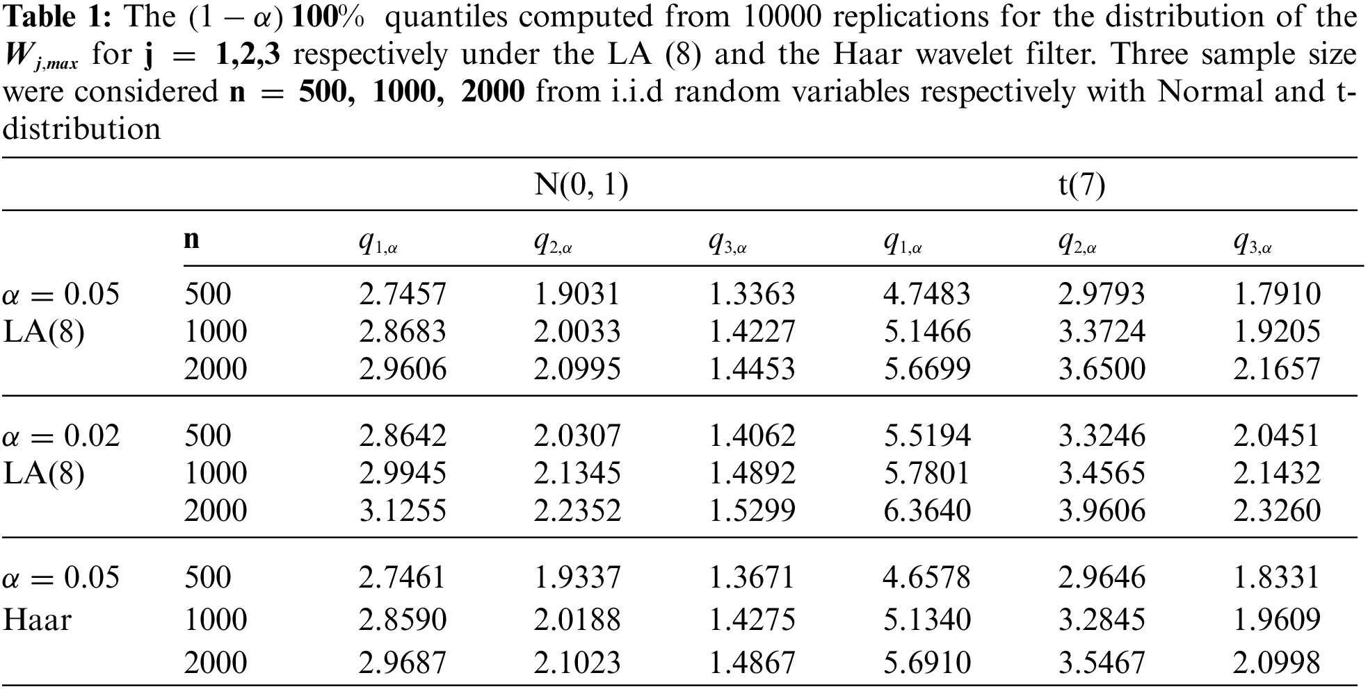
Our main focus now will be on detecting outliers in a time series by applying a threshold level on the maximum of the absolute value of the wavelets coefficients of residuals resulting from a GARCH type model. Using a Monte Carlo scheme, we can compute, for different sample sizes, the distribution of the maximum of the absolute value of wavelet coefficients resulting from the MODWT of i.i.d random variables following either a standard Normal or a Student’s t-distribution.

This paper is organized as follows: in Section 2 we present some GARCH Models with Outliers. In Section 3 we simulate the wavelet quantile thresholds from a Normal and Student t-distribution and describe the outliers detection procedure. Two real time series: the closed price series of respectively the Saudi stock market and S&P 500 index are processed. Their performances are discussed in Section 4, and conclusion is given in Section 5.

2  GARCH Model with Outliers

For illustration, our method is applied to several volatility models, such as the standard GARCH, the Exponential-GARCH (EGARCH) as defined in [16] and the Glosten, Jagannathan and Runkle-GARCH (GIR-GARCH) models in [17], with errors following either a Normal or a t-distribution. We can distinguish between two types of outliers as discussed in [9]. The additive outliers only affect the level we label as additive level outliers (ALO), and those that also affect the conditional variance labeled as additive volatility outliers (AVO). We consider in this study the effects of both the additive level outliers and additive volatility outliers. As a common practice in financial time series, we often work with returns due to their statistical characteristics and are unit-free. For time series Xt such that Xt>0 we consider the return series Rt defined by

Rt=100∗(ln⁡(Xt)−ln⁡(Xt−1))t=2,…,N(1)

2.1 Additive Level Outliers (ALO)

Assume that the series of returns is given by a standard GARCH (1, 1) model

Rt=μt+atwithat=σtεt(2)

where μt is the conditional mean and the volatility σt is such that

σt2=ω+α1at−12+β1σt−12(3)

where εt is an i.i.d. white noise. The parameters ω,α1andβ1 are such that

ω>0,α1≥0,β1≥0andα1+β1<1

An outlier of the type additive level is an outlier where the mean level of the time series changes at particular time, and then the series keeps evolving in the same way as previously. The conditional mean with additive level outliers (ALO) is defined as

Rt=μt∗+at=μ+μAIS(t)+at(4)

where μA is the magnitude of the additive level outlier at the unknown time s. IS(t)=1 for t∈S and 0 otherwise and S is the set of times when outliers are occurring. Note that in practice, the timing of the outlier s is often unknown.

2.2 Additive Volatility Outliers (AVO)

The additive volatility outliers (AVO) for the GARCH(1, 1) model is defined as

Rt=μt+at∗=μt+σt∗εt

at∗=μAIS(t)+atandσt∗2=ω+α1at−1∗2+β1σt−1∗2      t=1,2,…n(5)

where σt∗2 is affected by previous outliers and can be expressed in terms of outlier effect by replacing at∗ as follows:

σt∗2=ω+α1at−12+α1(2μADat−1+μAD2)IS(t−1)+β1σt−1∗2(6)

Note that Eq. (6) can be used to generate a GARCH(1, 1) with a set of outliers. On the other hand, in order to express the contaminated σt∗2 in term of the uncontaminated conditional variance σt2 given by Eq. (3), we first substitute at∗ from Eq. (5) to get

σt2=α0+α1∑j=1t⁡β1j−1at−j2whereα0=ω(1−β1t)/(1−β1)+β1tσ02(7)

Then it follows from Eqs. (3), (5) and (7) that

σt∗2=σt2+α1β1t−s−1  (2μAas+μA2)IS(t−1)(8)

Eq. (8) is also given by Eq. (8) in [10], and show that the effect of the outlier on the volatility diminishes over time. This means that the effect of the initial impact of the outlier is limited to the few subsequent observations, and the length of the impact depend on the model coefficients.

3  Outliers Detection

Let X=(X1,…,Xn) be an observed time series; then, by applying the MODWT to the series X, we obtain the wavelet coefficients Wj,1,Wj,2…,Wj,n at level j for j=1,2,…J. The main properties of wavelet coefficients Wj,t is their sensitivity to the existence of nonsmooth features in the data such as spikes and jumps in data, and more importantly, they remove any trend in the series. Motivated by such attractive properties, let define the maximum of the absolute value of these coefficients.

Wj,max=maxt|Wj,t|(9)

Unfortunately, the distribution of Wj,max is unknown and complicated, the critical values have to be calculated numerically. Using Monte Carlo simulation, we obtain the (1−α)100% quantiles given in Tab. 1 for the distribution of Wj,max for different sample sizes n of the series. For the sake of simplicity we restrict ourselves to the first few levels and in our case we run the procedure for j=1,2,3. In practice we can run for upper levels but we should bear in mind that the corresponding quantiles decrease in value as we move to higher levels.

3.1 Identification of Outliers

The outliers are identified as those observations in the series whose absolute value of wavelet coefficients exceed a threshold value which we set to be the (1−α)100 quantile qj,α of the distribution of Wj,max. This procedure can provide a soft approach to deal with outliers and help to remove outliers from the residuals that may invalidate the fitted model to the series and severely affect the model coefficients. We should note here that the quantiles in Tab. 1 are computed under the Least Asymmetric (LA(8)) wavelet filter for α=0.05 and α=0.02, and under the Haar wavelet filter for α=0.05. We can observe that these quantiles are nearly the same under the Normal distribution, but are also very close under the t-distribution which is similar to the Normal but with fatter tails.

3.2 Wavelet Quantile Distribution

The distribution of Wj,max resulting from an i.i.d sequence following either a standard Normal or a Student’s t distribution is depicted in Figs. 1 and 2 for the sample size of n=1000. These distributions are right heavy tailed distribution starting with larger values at lower scales and decrease as we move toward high scales. We should point out here that our quantiles under the Haar filter are all smaller than those obtained in [6]. This is because they use details of the standard DWT instead of the wavelet coefficients obtained from the MODWT as in our case. Both quantiles obtained under the LA(8) and the Haar wavelet are very close. This shows that there are not very sensitive to wavelet shape and length under the t-distribution. The Haar wavelet filter is the shortest filter and the LA(8) which belong to a family of filters is of moderate length and considered as against artifacts. In practice, different wavelet filters can be applied to achieve a wavelet decomposition and generally one should try different wavelet filters. Although our computed 95% quantiles show no dependency to the filter being used LA(8) or the Haar filter under both distributions Normal and t-distribution. This should not be misinterpreted and consider that the choice of the wavelet filter is irrelevant. In practice when analyzing time series data using DWT or the MODWT, we should apply wavelet filters of moderate lengths, with compact support and higher order of vanishing moments to avoid artifacts as discussed in [15], and this is where the LA(8) is recommended over the Haar filter.

Figure 1: Histograms computed from 10000 replication for the distributions of Wj,max resulting from the MODWT with LA (8) filter applied to i.i.d standard Normal with sample size n=1000

Figure 2: Same as Fig. 1 but applied to an i.i.d sequence from the Student t-distribution with sample size n=1000

3.3 Methodology

We propose the following steps of the procedure to detect additive outliers in a GARCH model:

(1)   Fit a volatility model, such as a GARCH, EGARCH or GJR-GARCH to the returns Rt

(2)   Set the J-level wavelet transform as J. Let Wj,t be the j-level wavelet coefficient of the series of residuals at∗ resulting from the fitting in step (1).

(3)   Find the maximum value Wj,k(obs)=maxt⁡{|Wj,t|>qj,α} where k is the index of the maximum of absolute value of the observed wavelet coefficient and qj,α is the applied threshold level.

(4)   Set Wj,k(obs)=0 and reconstruct the residual series to obtain a1,t∗ using the IMODWT

(5)   Set the new series of returns as R1,t=μt+a1,t∗

(6)   Steps (1)-(5) can be repeated by increasing the J-level until no further outliers are left.

The above procedure can be applied to any GARCH like model.

4  Results and Discussions

In order to measure the performance of the above procedure on real data, we consider two financial return series. The closed price series of the Saudi Stock market of length 2027 over the period Aug. 10 2011 to Dec. 31 2019 described in [18], and the S&P 500 index of the closed price series over the period Jan. 05 2006 to Oct. 26 2012 of length 1717. The S&P 500 data is available from https://www.investing.com/indices/us-spx-500-historical-data. Note that when running our outliers removal procedure we apply the MODWT using the wavelet filter LA(8) for both series.

4.1 The Saudi Stock Market Closed Prices

The descriptive statistics of the returns Rt show an excess kurtosis of 10.7504 larger than the Normal value of 3.0. This finding of excess positive kurtosis shows that the distribution tails of the returns series are “fatter” than the Normal distribution, and hence this can be regarded as evidence that support the presence of outliers.

4.1.1 The Conditional Mean

The returns series Rt has a non-constant variance and high variability between 2014 and 2016. The autocorrelation sample (ACF) of Rt and its square Rt2 are shown in Fig. 3, a) and b) respectively. The estimated autocorrelation coefficient of Rt at lag 1 is well outside the test bounds, which suggest an AR(1) model for the mean of the series. Also the ACF of the squared series Rt2 shows that they are many lags that are well outside the test bounds. The amount of dependence displayed by the series Rt2 is important. This is considered as evidence that support the use of an appropriate GARCH like model to account for the amount of this autocorrelation. On the other hand the Quantile-Quantile plot (QQ-plot) in Fig. 3, c) confirms that Rt does not come from a Normal distribution and suggest a fat-tail distribution.

Figure 3: The sample ACF of Rt and its square Rt2 respectively in a) and b), and c) the sample quantile QQ-plot relative to the normal distribution of Rt

4.1.2 Volatility Modeling

Three class of GARCH models are considered in the analysis of the returns series, mainly the standard GARCH (1, 1), the exponential EGARCH (1, 1) which models the logarithm of σt2 and expected to capture the effect of external shocks on the predicted volatility, and the GIR-GARCH(1, 1) which is expected to observe the fact that negative shocks at time t−1 have a stronger impact on the variance at time t than positive shocks which is known as the leverage effect. The conditional variance σt2 in these GARCH type models depends on the lagged squared residuals as well as on lagged conditional variances.

Tab. 2 summarizes the main parameters and their p-values for the three GARCH models fitted to the return series Rt under the t-distribution before removing any outliers. The last two columns of the Tab. 2 give the root mean square error (RMSE) and the root mean absolute error (RMAE) as a measure of forecast accuracy computed on the basis of out-of-sample data.

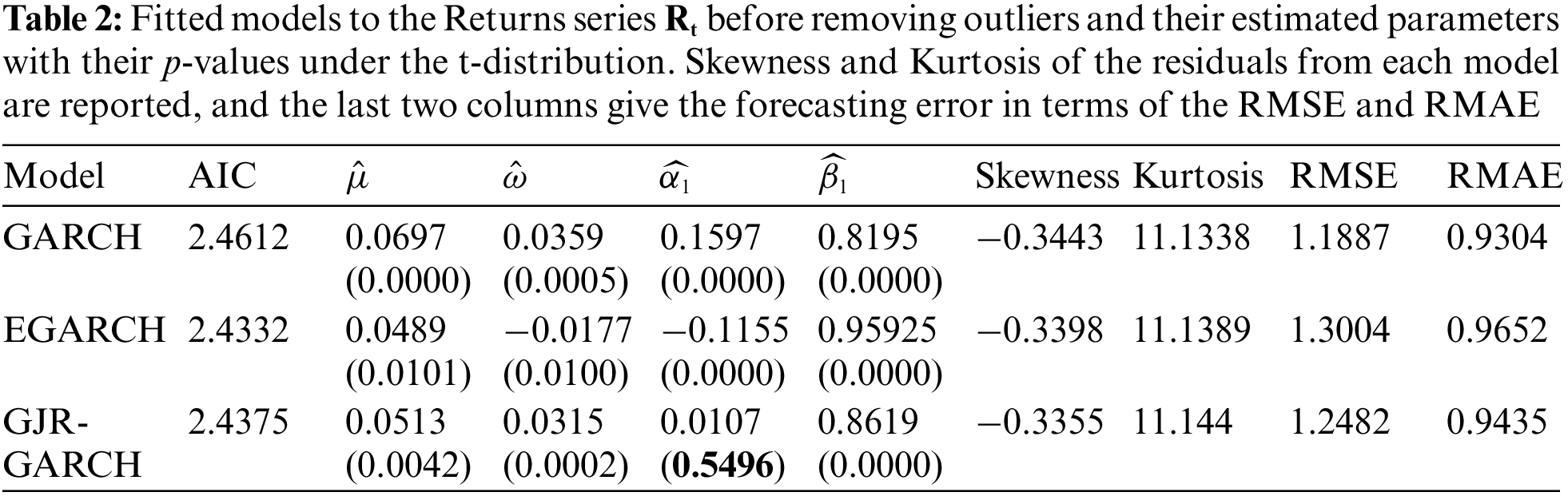
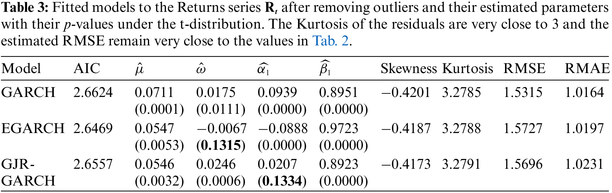
We can easily see that the GARCH (1, 1) achieves the best performance, and EGARCH (1, 1) is of acceptable performance under the t-distribution. However, the Kurtosis values of residuals of both models are over 11.0. This indicates excess of positive kurtosis and hence the presence of heavy tail distribution in the residuals which is very likely due to the presence of outliers in the return series. The returns are then subject to the procedure as described in the methodology. After running the procedure steps, we summarize in Tab. 3 the parameter estimates in the three models. The GARCH (1, 1) realizes the best performance, and the Kurtosis value of all three models is around 3 which is very close to the one of Normal distribution. This is a strong evidence that the presented wavelet based procedure removes the effect of outliers and allow for a much better modelling of the return series. We should also note that similar results can be drawn under the asymmetric t-distribution but without any improvement.

4.1.3 A Lower Hard Threshold

Although satisfied by the results in Tab. 3, the residuals distribution analysis in term of the QQ-plot still displays outliers. This can be explained by the fact that some threshold quantile used as threshold for outliers are larger as given in Tab. 1, particularly at lower levels of the wavelet transform. Hence not all larger residual values are discarded, and this is more likely to occur if the probability distribution of the residuals does not match the distribution under which the quantile threshold were computed. Now one of the attractive properties of the MODWT wavelet transform is that the wavelet coefficients at higher level of the transform get smoother, smaller in magnitude and their expected values are such that E(Wj,t)=0. As an empirical rule we suggest to use the higher j-level wavelet quantile threshold for lower j-level wavelet coefficient of residuals. Obviously using this approach, we certainly face the problem of how do we choose these higher j-level wavelet threshold quantile. In our Saudi Stock returns series example, we used the lowest quantile threshold as the single common hard threshold. This correspond to the higher level J=3 in our case. The results given in Tab. 4 show that the Kurtosis are getting smaller around the value 1.0 which means that the residuals distribution is platykurtic and has fewer and less extreme outliers than does the normal distribution. We can notice and improvement in term of the overall goodness of fit of GARCH models and their residuals.

4.2 The S&P 500 Index of the Closed Prices

The methodology is also applied to the S&P 500 Index series which is downloaded from investing.com. The time period of analysis is over 6 years and 10 months. Returns were computed from the original series of the closed prices. Fig. 4 represents the original series and the returns. It can easily be observed that the series is not stationary and displays a high variability over the period 2008–2009 which is also displayed by the presence of larger and smaller returns over the same period.

The autocorrelation sample ACF of Rt and its square Rt2 are shown in Fig. 5, a) and b). The estimated autocorrelation coefficient of Rt suggest an AR (1) model for the mean of the series. Also the ACF of the squared series Rt2 shows a very similar pattern as in Fig. 3. The serial dependence displayed by the series Rt2 is important and taken as evidence that support the use of a GARCH like model to account for this autocorrelation. This is also comfirmed by the QQ-plot in Fig. 5, c) which suggest a fat-tail distribution and indicates the presence of outliers in the Rt series

Figure 4: a) The S&P 500 series between Jan. 05 2006 to Oct. 26 2012, and b) The returns series Rt

Figure 5: The sample ACF of Rt and its square Rt2 respectively in a) and b), and in c) the sample quantile QQ-plot relative to the normal distribution of Rt

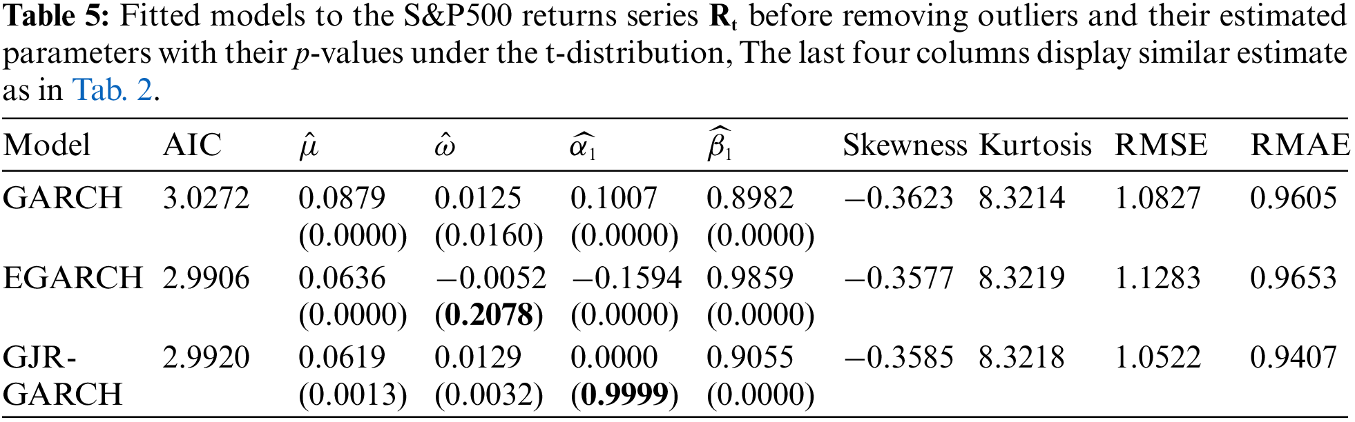
Tab. 5 summarizes the results obtained from the three GARCH models. It can be observed that the GARCH (1, 1) model provides good performance relatively to the other models under the t-distribution. We should point out here that by allowing a Normal or the asymmetric t-distribution it was not possible to achieve similar performance. On the other hand the larger positive kurtosis values in the residuals are regarded as evidence for the presence of extreme values such as outliers.

By applying the wavelet based procedure to the returns Rt, it can easily be observed that the effect of such outliers is removed and this is comfirmed by the small estimated Kurtosis values down from 8.32 to 1.44 as given in Tab. 6. This means that the residuals distribution is platykurtic which in turn indicates they have light tails and lack of outliers.

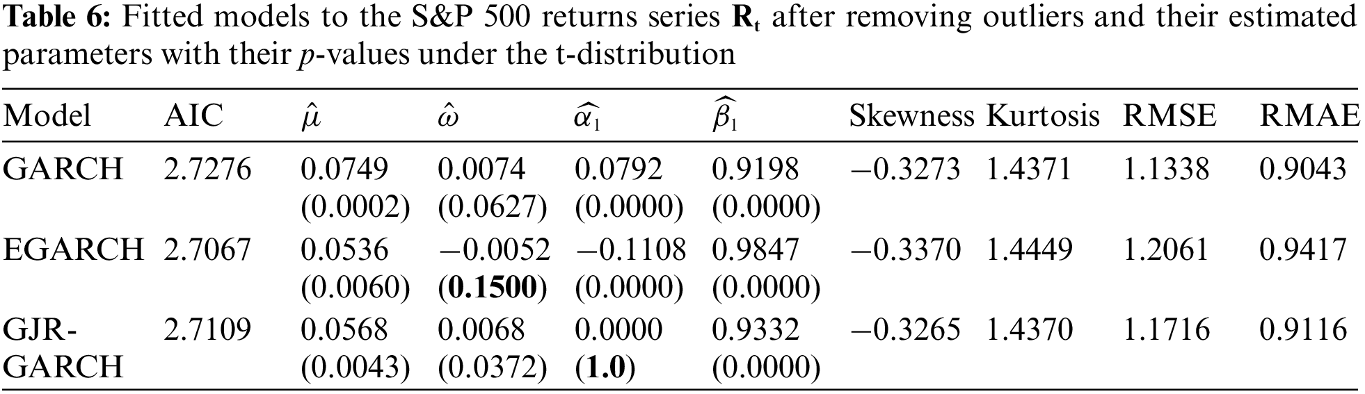
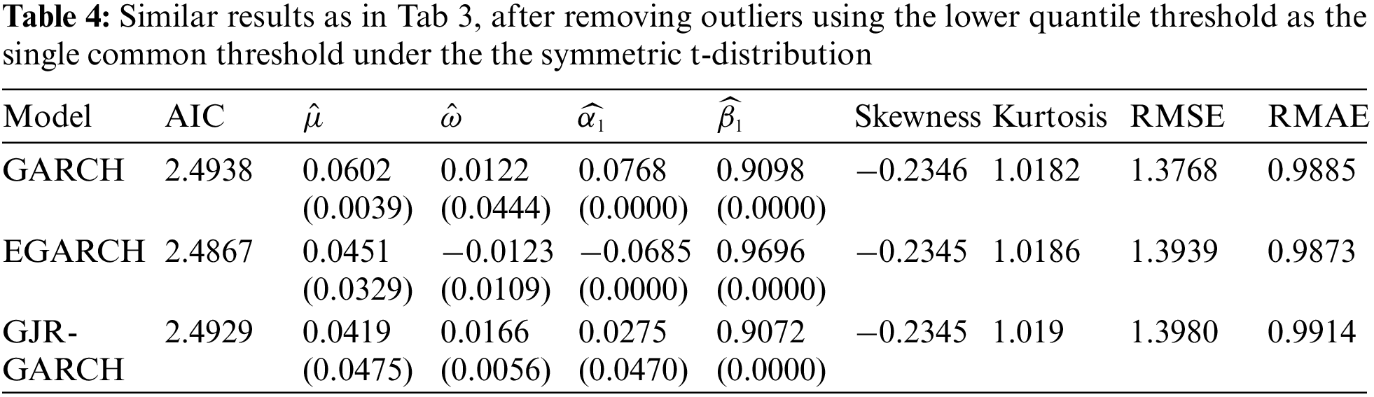
In contrast to the first series, because of the small Kurtosis values in Tab. 6 there is no need to apply a lower hard threshold. Thus when applied to the S&P500 returns series it did not really improve the goodness of fit for all models, but it did remove some few values of very small magnitude from the residuals.

5  Conclusion

Our MODWT wavelet coefficients based detection of outliers is applied to two real financial dataset: the closed price of the Saudi Stock market and the S&P500 returns series. The outliers detection approach make use of the maximum of the absolute value of these wavelet coefficients as described in the procedure. Using “rugarch” the R package we fitted the standard GARCH (1, 1), EGARCH (1, 1) and GJR-GARCH (1, 1) models to each series as given in Tabs. 2 and 5. None of the original series is stationary and the estimated residuals Kurtosis from each series strongly suggest the presence of outliers. By applying our procedure separately to each series, the results of Tab. 2 show that the GARCH(1, 1) model was selected as the best fit to the Saudi Stock returns, but their residuals still show excess of Kurtosis, and certainly do not behave as a white noise. This is evidence that the fit did not quite capture the structure in the data, and the residuals were submitted to the outliers detection procedure. Tab. 3 shows that after removing outliers from wavelet coefficients of residuals, the reconstructed returns still show a slight excess in Kurstosis, but was down from 11.1338 to 3.278 which is a big improvement. The new GARCH(1, 1) model was again selected as the best fit. Further analysis of the residuals show that their QQ-plot displays a slight mismatch between the fitted t-distribution and the true unknown distribution of errors. Tab. 4 shows an improvement in the residuals after applying the lowest hard threshold as the single common threshold and both models GARCH (1, 1) and EGARCH (1, 1) provide a good fit for the new reconstructed series of returns. For the second returns series we went through the same procedure before and after removing outliers. Tab. 6 shows that the GARCH(1, 1) model perform well after removing the outliers. On the contrary to the previous example the use of the lowest hard threshold as the single common threshold did not add any improvement in the performance of the fitted model. This should not be very surprising given the small Kurtosis values in Tab. 6.

The proposed procedure is a promising addition to existing methods for detecting outliers in a general discrete time series models, where the focus is on the analysis of the residuals.. The two real data examples illustrate that our procedure is very successful in detecting outliers in financial time series.

Acknowledgement: We would like to thank the anonymous referees for their useful comments and efforts towards improving the quality of this manuscript.

Funding Statement: The authors received no specific funding for this study.

Conflicts of Interest: The authors declare that they have no conflicts of interest to report regarding the present study.

References

 1.  R. Engle, “Autoregressive conditional heteroskedasticity with estimates of the variance of UK. inflation,” Econometrica, vol. 50, pp. 987–1008, 1982. [Google Scholar]

 2.  T. Bollerslev, “Generalized autoregressive conditional heteroskedasticity,” Journal of Econometrics, vol. 31, pp. 307–327, 1986. [Google Scholar]

 3.  T. Bollerslev, “A conditionally heteroscedastic time series model for speculative prices and rates of return,” Review of Economic and Statistics, vol. 69, pp. 542–547, 1987. [Google Scholar]

 4.  R. Baillie and T. Bollerslev, “The message in daily exchange rates: A conditional variance tale,” Journal of Business and Economic Statistics, vol. 7, pp. 297–309, 1989. [Google Scholar]

 5.  T. Terasvirta, “Two stylized facts and the GARCH (1, 1) model,” in Working Paper 96, Stockholm School of Economics, 1996. [Google Scholar]

 6.  A. Gran´e and H. Veiga, “Wavelet-based detection of outliers in financial time series,” Computational Statistics and Data Analysis, vol. 54, pp. 2580–2593, 2010. [Google Scholar]

 7.  A. Blázquez-García, A. Conde, U. Mori and J. A. Lozano, “A review on outlier/anomaly detection in time series data,” ACM Computing Surveys, vol. 5, no. 3, pp. 1–33, 2022. https://doi.org/10.1145/3444690. [Google Scholar]

 8.  A. Grané and H. Veiga, “Outliers, GARCH-type models and risk measures: A comparison of several approaches,” Journal of Empirical Finance, vol. 26, pp. 26–40, 2014. http://dx.doi.org/10.1016/j.jempfin.2014.01.005. [Google Scholar]

 9.  L. K. Hotta and R. S. Tsay, “Outliers in GARCH processes,” in Manuscript, Graduate School of Business, University of Chicago, 1998. [Google Scholar]

10. J. A. Doornik and M. Ooms, “Outlier detection in GARCH models,” Tinbergen Institute discussion papers, 092/4, 2005. [Google Scholar]

11. M. T. Ismail, M. and I. N. M. Nasir, “Outliers and structural breaks detection in volatility data: A simulation study using step indicator saturation,” Discovering Mathematics (Menemui Matematik), vol. 42, no. 2, pp. 76–85.  2020. [Google Scholar]

12. I. N. M. Nasir, M. T. Ismail and S. A. A. Karim, “Malaysian tapis: A closer look into additive outliers and persistence volatility,” Journal of Physics: Conference Series, IOP Publishing, vol. 1123, pp. 012041, 2018. https://doi.org/10.1088/1742-6596/1123/1/012041. [Google Scholar]

13. I. N. M. Nasir and M. T. Ismail, “Detection of outliers in the volatility of Malaysia shariah compliant index return: The impulse indicator saturation approach,” ASM Science. Journal, vol. 13, pp. 1–7, 2020. [Google Scholar]

14. K. A. Rashedi, M. T. Ismail, S. A. Wadi and A. Serroukh, “Outlier detection based on discrete wavelet transform with application to Saudi stock market closed price series,” The Journal of Asian Finance, Economics, and Business, vol. 7, no. 12, pp. 1–10, 2020. [Google Scholar]

15. D. Percival and A. Walden, “Wavelet Methods for Time Series Analysis,” New York: Cambridge University Press, 2000. [Google Scholar]

16. R. F. Engle and K. N. G. Victor, “Measuring and testing the impact of news on volatility,” The Journal of Finance, vol. 48, no. 5, pp. 1749–1778, 1993. [Google Scholar]

17. L. Glosten, R. Jagannathan and D. Runkle, “On the relation between the expected value and the volatility of the nominal excess return on stocks,” Journal of Finance, vol. 48, no. 5, pp. 1779–1801, 1993. [Google Scholar]

18. T. S. Al Shammary, M. T. Ismail, S. AL-Wadi, M. H. Saleh and J. J. Jaber, “Modeling and forecasting Saudi stock market volatility using wavelet methods,” Journal of Asian Finance, Economics and Business, vol. 7, no. 11, pp. 83–93, 2020. [Google Scholar]

This work is licensed under a Creative Commons Attribution 4.0 International License, which permits unrestricted use, distribution, and reproduction in any medium, provided the original work is properly cited.