DOI:10.32604/cmc.2022.023453
| Computers, Materials & Continua DOI:10.32604/cmc.2022.023453 | |
| Article |
A New Fuzzy Controlled Antenna Network Proposal for Small Satellite Applications
Taif University-Khurma Univ., College-Department of Computer Sciences, Khurma, 2935, Kingdom of Saudi Arabia
*Corresponding Author: Chafaa Hamrouni. Email: cmhamrouni@tu.edu.sa
Received: 09 September 2021; Accepted: 18 November 2021
Abstract: This research contributes to small satellite system development based on electromagnetic modeling and an integrated meta-materials antenna networks design for multimedia transmission contents. It includes an adaptive nonsingular mode tracking control design for small satellites systems using fuzzy waveless antenna networks. By analyzing and modeling based on electromagnetic methods, propagation properties of guided waves from metallic structures with simple or complex forms charge partially or entirely by anisotropic materials such as metamaterials. We propose a system control rule to omit uncertainties, including the inevitable approximation errors resulting from the finite number of fuzzy signal power value basis functions in antenna networks. Moreover, both the stability and the tracking performance of the closed-loop robotic system are experimentally validated. The research lies within the scope of the improvement of speed, effectiveness, and precision of numerical methods applied to electro-magnetic modeling with complex structures, essentially rectangular metallic waveguides filled with isotropic or anisotropic metamaterials. Three axes of our research are presented: waveguides, filters, and antennas. The proposed controller does not require prior knowledge about the dynamics of the fuzzy system controller for antenna networks or the offline learning phase. In addition, this work contributes to solving the problem of non-visibility stations to ensure data transmission in wireless networks. The proposed solution maximizes inter-connection by using a fuzzy controlled antenna network, and the novelty guarantees non-limited interconnection in wireless networks compared to traditional methods.
Keywords: Metamaterials; ferrites; complex modes; discontinuities; antennas; ultra-wide band; MATLAB; advanced design system
Human reasoning can be based on inaccurate or incomplete data, while computers only process exact data. The theory of logic was introduced by Zadeh in 1963 to solve part of the problem and touch the fuzzy approaches of the meadow [1]. This section deals with concepts related to the proposed fuzzy control system, whose objective is to integrate it on board the picosatellite [2]. Fuzzy logic is born from the observation that most phenomena cannot be represented by Boolean variables that only use “0” or “1” to describe things. To answer this type of question, such as “Can a power of 0.6 W be considered low or high?” and “Is not she weak or really high but just average?” [3], fuzzy logic considers the belonging notion of an object to a set, replacing the Boolean function with a function with continuous values between 0 and 1. The development of multimedia system technology is mainly based on the innovation of hardware and software systems, so system interconnection should be carefully studied. The challenges for the development of multimedia technology mainly rely on the development of communication networks, especially wireless networks [4]. We contribute to developing antenna technologies and improving their efficiency. Our contribution in this context is to propose a new fuzzy controlled antenna network proposal for small satellite applications. This idea is added to maximize wireless interconnection duration, as well as stations for multimedia transmission contents. The work aims to find a solution for antennas related to multimedia center interconnection with targets. Traditional centers are characterized by a limited visibility angle that affects the amount of multimedia transmission data. Then, we use a simulation tool based on MATLAB script functional programming [5], where MATLAB is one of the most widely used high-level programming languages for scientific and engineering computations.
2 Elements of the Fuzzy Logic Rule
The interest of fuzzy logic lies in its ability to simplify the realization and use of computer applications. It allows the replacement of mathematical models by models based on verbal descriptions [6,7]. Regarding the control of any process, fuzzy logic allows a founding approach compared to the conventional automatic. In automatic, in general, we try to model the process through a certain number of differential equations. It is very user-friendly and does not need practically formal programming knowledge. We learn MATLAB programming aspects and commands from scientists and engineers with formal programming training and spend significant time programming to solve our real-world problems. The MATLAB seminar covers the functional and script programming of the MATLAB language. We use specific expectations to recognize MATLAB commands, scripts, and functions. Then, we create and run a MATLAB function. Next, we read, recognize, and describe MATLAB syntax. Finally, we realize decisions, loops, and matrix operators. We evaluate scopes among multiple files and multiple functions within a file. However, this is difficult for modeling, and sometimes it is impossible to measure the complexity of processes. In a radically different way, a controller does not focus on how to describe the process but on how to control it, just as a human expert follows the rules and introduces some inaccuracies and/or uncertainties [8]. The main concepts of fuzzy control are essentially divided into two main parts: 1) the sets, fuzzy variables, and associated operators, and 2) the decision-making from a base “If-Then” rule. Thus, different steps of achieving a fuzzy command can be represented in Fig. 1.
Theoretically, an element either does or does not belong to a set. The notion of the ensemble is at the origin of many mathematical theories. The binary variables are defined by two states, “true” or “false”, and the fuzzy variables have a gradation between the value “true” and the value “false”. However, the essential notion does not make it possible to account for simple and frequently encountered situations. It takes into account such situations that the notion of a fuzzy set has been created. The theory of fuzzy sets is based on the notion of partial membership: each element partially or gradually belongs to the fuzzy sets, defined in [9]. Mathematically, we can determine the fuzzy set A of the universe X by applying A of X in the interval [0,1]. For each element
The function

Figure 1: Main diagram of fuzzy controller system
The muddling capacity can be utilized to safeguard the area security of individuals while speaking with local-based services for discovering areas of its advantage. The confusion is the defect of purposeful corruption of spatial data quality. The defect recorded in writing may be imprecision, error, and unclearness. Imprecision is the absence of particularity in data. Error is the absence of correspondence among data and reality, while unclearness in data identifies with limited cases. The defect can be utilized for confusion capacity to safeguard the area security. The fundamental security quality of jumbling is the property of reversibility, which makes it hard for an enemy to figure out the muddled informational index. Confusion can additionally give staggered information security dependent on different requests of end clients. Anonymization-based systems have the issue of verification and personalization, while the muddling system improves the assurance level of area security. A muddling system does not rely upon focal regulators to manage protection strategies, making it reasonable for appropriated conditions. The structure security investigation perspective expresses that a muddling system is produced to give more significant levels of area security insurance. It is a troublesome undertaking to amass a higher number of clients in a concerned territory without standing. We use obscurity capacity to safeguard the area protection and establish a relationship between the truth degree of the fuzzy variable and the corresponding input quantity. When talking about fuzzification, the values taken to trace the membership function in Fig. 2 are the experimental results of the system to be controlled: this is the opinion of the expert. In our study, the most used membership functions, trapezoidal and triangular functions, are used.

Figure 2: Membership functions. (a) Trapezoidal function form. 1, (b) Trapezoidal function form. 2, (c) Triangular function
The use of membership functions defines the system control for deciding on how it operates. This point is essential for system result analysis and future tasks, such as maintenance. The small satellite antennas operate in real time, but the selection of the suitable antenna is accomplished by the optimized membership function adopted in the system. A fuzzy controller is a universal tool for decision-making when values are similar. The small satellite application of machine learning and deep learning techniques for antenna network optimization represents the latest research trend. But the data and measurement values are huge to store. This algorithm presents minuses time for decision-making and omits all steps for deep learning techniques, as well as machine learning, which necessitates memory hardware and operating time.
The equation of the curve is in the form1:
The equation of the curve is in the form2:
The equation of the Triangular function is as follows:
These fuzzy intervals (Tab. 1) define the number of fuzzy variables associated with an input quantity. These intervals are given by an expert following his experiments on a controlled system. In the case of adjustment, three to five intervals are sufficient. As the antennas are intended to be mounted on the faces of the pico satellite, i.e., an antenna on each side, a fuzzy controller with six inputs and six outputs has been provided. This choice has been adopted for a purpose. We maximize the probability of having at least one antenna opposite the earth station. The inputs X, Y, Z, T, W, and U go through different phases in the controller: fuzzification, inference, and defuzzification. The outputs are SX, SY, SZ, ST, SW, and SU. These elements are characterized by symbols presented in Tab. 1.

2.3 Rules of Inference and Operators
These rules are used to connect fuzzy input variables to fuzzy output variables using different operators. They must be defined by a system control expert according to his experience (expert role) and stored in a control unit.
- Combination of rules: The set of rules is in the form of an enumeration type. If condition.1 and/or condition.2, then Action on the outputs. The combination of these different rules is done using an OR operator. The justification of the operator choice is based on the practice of the current language. So an enumeration is understood in the sense of “If …. Then” or “Si … Then”.
- Operators: The inference rules use the operators (Tab. 2) “And”, “Or”, and “Not”, which apply to the fuzzy variables. In the case of binary logic, these operators are defined in a simple and unambiguous way. In the case of fuzzy logic, the definition of these operators is no longer univocal, and the relations presented in Tab. 2 are most often used [10].

The minimum and maximum operations have the advantage of simplicity when calculating. However, they favor one of the two variables. Product operations and average values are more complex to calculate but produce a result that considers the values of two variables, see Fig. 3.

Figure 3: Graphics of operators. (a) Operator NOT, (b) Operator NOT, (c) Operator AND
Operator Not
A NOT operator is called “complement”, “negation”, or “inverse”:
a-Mechanism of Inference and Defuzzification
Different rules of inference produce a value. These different values must be combined according to a mechanism in order to obtain the (possible) output variable(s). Then the fuzzy variable(s) of output must be converted into a control variable (voltage, torque, etc.) in order to be applied to adjust the system. This last stage is called defuzzification [11].
b-Inference Mechanisms
The inference mechanism calculates the fuzzy subset μ (x0) relative to the control of the system. In the fuzzy logic controller, inference intervenes the operators “AND” and “OR”. The AND operator applies to variables within a rule, while the OR operator binds different rules. One of the following methods is generally used for the adjustment by fuzzy logic: the Max-Min inference method, the Max-Prod inference method, and the Sum-Prod inference method. In the following, we will use the Max-Min inference method.
c-The Max-Min Inference Method
At the condition level, this method realizes the operator OR by the maximum formation and the operator AND by the minimum formation. The conclusion in each rule, introduced by THEN, links the condition's membership factor with the output variable's membership function by the AND operator, realizing in the present case by the minimum formation. Finally, an OR operator that binds the different rules is realized by the maximum formation [12]. In the previous example, the inference is as shown in Fig. 4.
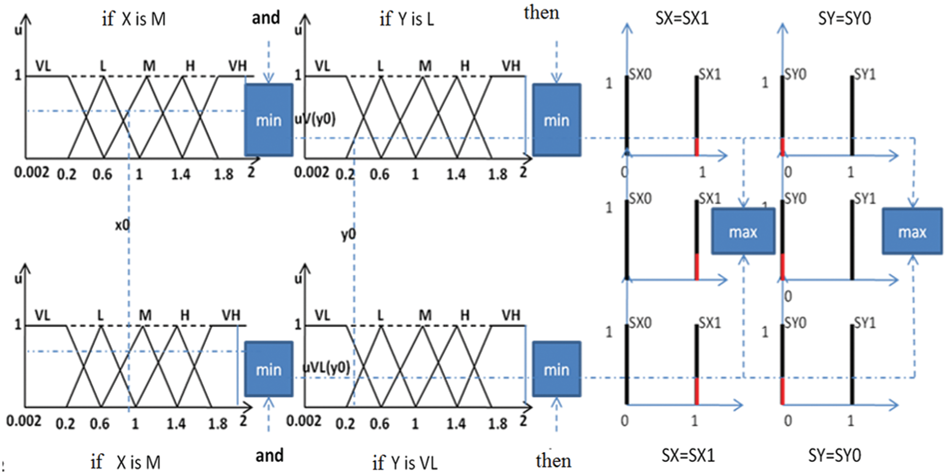
Figure 4: The max-min inference method
d-Defuzzification
The inference engine provides a resulting membership function for the output variable. It is, therefore, fuzzy information. Since the controller requires a precise control signal at its input [13,14], it is necessary to transform this fuzzy information into specific information, which is called defuzzification [15]. There are several methods for calculating the representative value of an output set, and the main ones of which are:
- Defuzzification by calculating the center of gravity.
- Defuzzification by calculation of the maximum
The Center of the Gravity Method
The most used defuzzification method determines the gravity center of the resulting membership function μRES(z). It is used when fuzzy intervals of the output contain multiple values. In this context, it is sufficient to calculate the abscissa z by the following formula:
The Maximum Method
This is the simplest met.
This is the simplest method avoiding the heavy calculation of the center of the gravity method.
This is the simplest method avoiding the heavy calculation of the center of the gravity method. For the output signal z*, the abscissa of the maximum value of the resulting membership function μRES (z) is chosen. This method is widely used when the fuzzy intervals of the output are discrete. The tools provided by fuzzy logic allow modeling phenomena that can come closer to human reasoning in a certain sense. Going beyond all or nothing of computers introduces flexibility, making the power of fuzzy tools in many fields.
2.3.2 The Fuzzy Controller with Six Inputs and Six Outputs
There is a fuzzy controller with six inputs and six outputs in Fig. 5. The inputs X, Y, Z, T, W, and U go through different phases in the controller: fuzzification, inference, and defuzzification. The outputs are SX, SY, SZ, ST, SW, and SU.
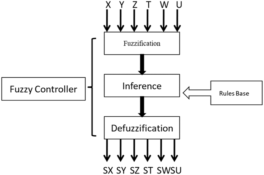
Figure 5: The structure of the fuzzy controller with six inputs and six outputs
Fig. 5 represents the central point for problem-solving related to small satellite applications and antennas. Signals representing data from multimedia transmission content will be quantified and evaluated.
a-Inputs and Outputs
• X: an input variable, a power varies between 0.002 and 2 W.
• Y: an input variable, a power varies between 0.002 and 2 W.
• Z: an input variable, a power varies between 0.002 and 2 W.
• T: an input variable, a power varies between 0.002 and 2 W.
• W: an input variable, a power varies between 0.002 and 2 W.
• U: an input variable, a power varies between 0.002 and 2 W.
• SX: an output variable, defining the choice of X, either “0” or “1”.
• SY: an output variable, defining the choice of Y, either “0” or “1”.
• SZ: an output variable, defining the choice of Z, either “0” or “1”.
• ST: an output variable, defining the choice of T, either “0” or “1”.
• SW: an output variable, defining the choice of W, either “0” or “1”.
• SU: an output variable, defining the choice of U, either “0” or “1”.
b-Fuzzification
At the Fuzzification phase in our case, the system performs various steps in the turnstile. It must wait for the response of FEED_BACK to restart the input stream processing and the fuzzification simulation results of Input variables. This step calculates the membership degree of each input value to the fuzzy sets, assigning n values of μ for each variable (n: the number of system rules). This task is done simultaneously.
Combination of rules: calculating the result μ of each rule. This task is done successively.
Inference: grouping the result μ according to the rules.
In the phase of defuzzification, we calculate the Maximum output value and choose the most important output as the final output of the system. Then, we send a FEED_BACK to the fuzzification stage to restart the process. For a classic model of the fuzzy controller, after the definition of inputs and outputs and the code implementation in its kernel, it is impossible to change the operation of the controller. The results of the simulation phase of output variables are shown in Fig. 6.
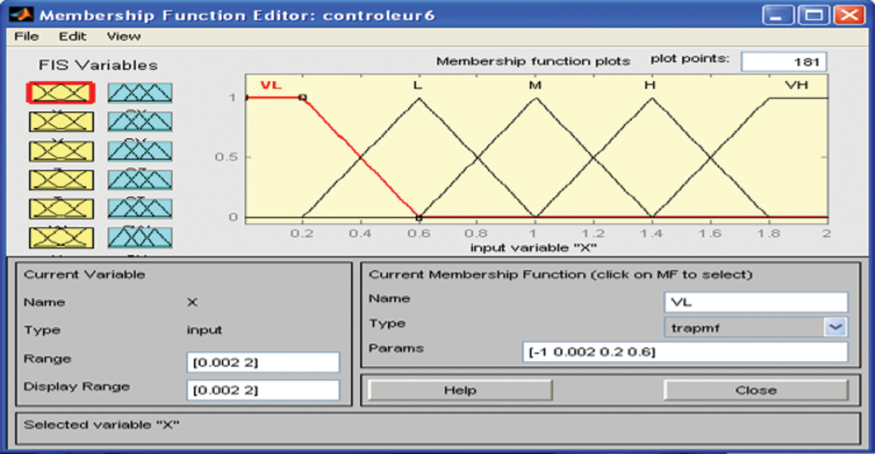
Figure 6: The membership feature editor (simulation)
At the moment t in the system operation, one or more ports fail, or the power is zero. The system does not work, and it goes into the waiting phase for six inputs as presented in Fig. 7, resulting in an unreliable system.
c-Input Fuzzification Variables
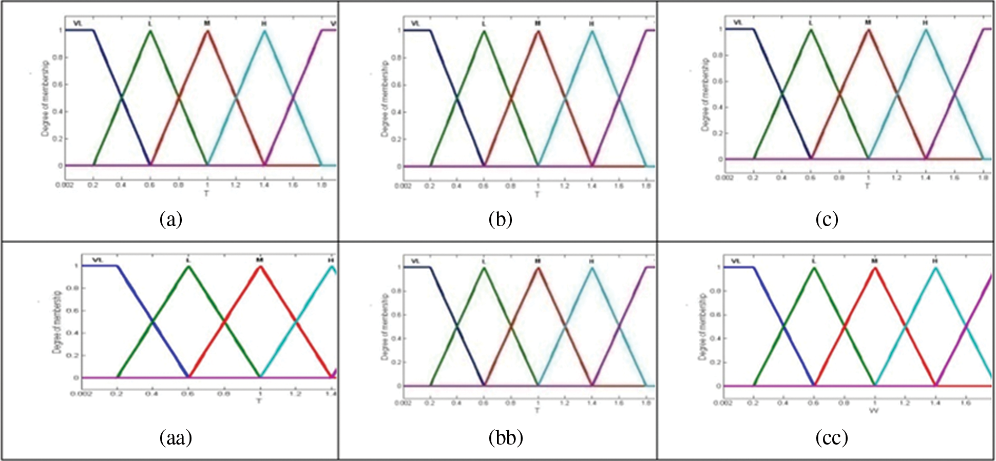
Figure 7: The fuzzification graph of input variables (simulation). (a) Input variable fuzzification x, (b) Input variable fuzzification y, (c) Input variable fuzzification z, (aa) Variable fuzzification of input t, (bb) Fuzzification variable of input w, (cc) Fuzzification variable of input u
d-Output Fuzzification
Outputs values are “0” or “1” in Fig. 8.
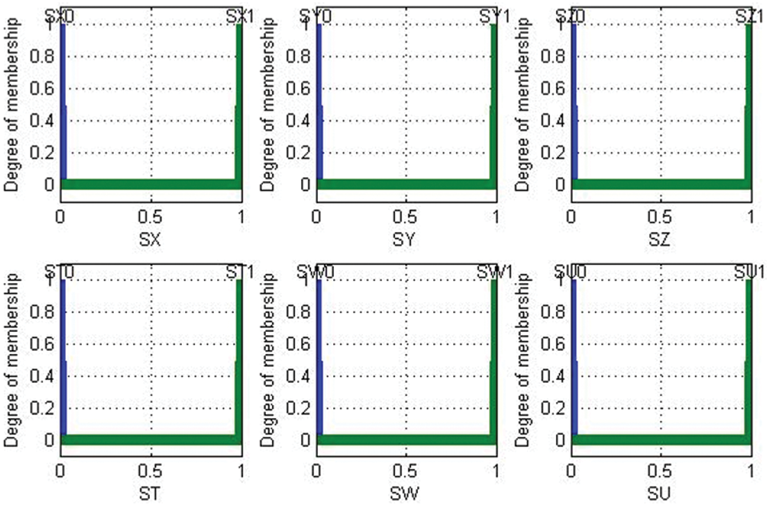
Figure 8: Fuzzification of outputs SX, SY, SZ, ST, SW, and SU
e-Rules of Inference
The base of fuzzy controller rules is built according to the following algorithm:
• The choice is made on the highest power;
• If the powers are equal and achieve maximum, we choose the first maximum. (if X = Y = Z = T = W = U, then choose X).
f-Inputs and Outputs
Surface of decision
For each output, there are 15 decision surfaces with respect to inputs in Fig. 9. In total, we have 15 * 6 = 90 surfaces.
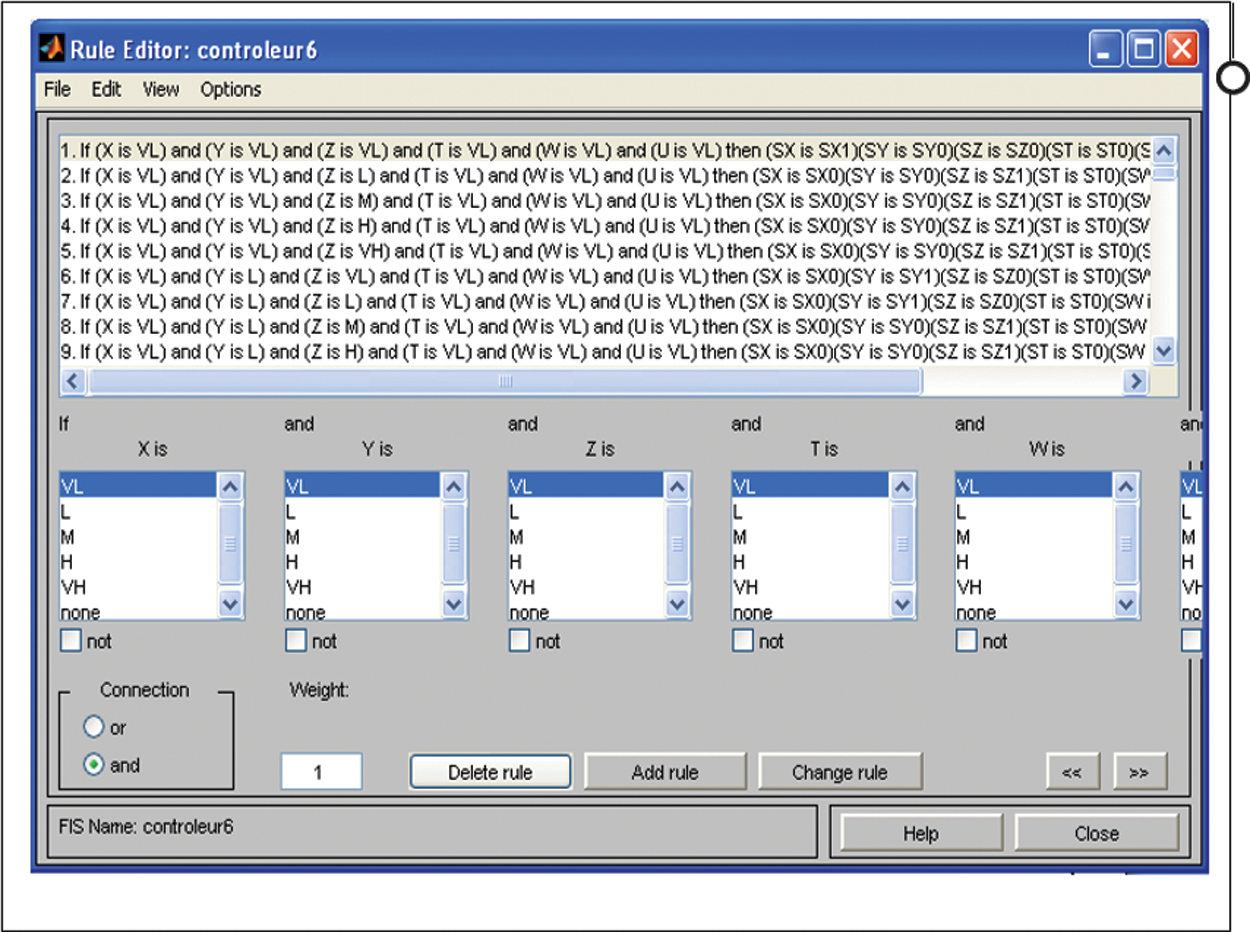
Figure 9: The rule editor: six inputs and six outputs (simulation)
For the Output SX
Fig. 10 represents decision-making based on system output evaluation. For each output, we have 15 decisions represented by surfaces. All decisions are made based on input evaluation. We have 90 surfaces that mean 90 decisions. For each output, there are 15 decision surfaces with respect to the inputs. In total, we have 15 * 6 = 90 surfaces.
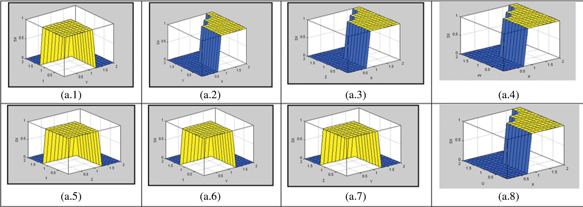
Figure 10: Decision surfaces (simulation). (a.1) Decision surface of sx with respect to x and y, (a.2) Decision surface of sx with respect to x and z, (a.3) Decision surface of sx with respect to x and t, (a.4) Decision surface of sx with respect to x and w, (a.5) Decision surface of sx with respect to x and u, (a.6) Decision surface of sx with respect to y and z, (a.7) Decision surface of sx with respect to y and, (a.8) Decision surface of sx with respect to z and t
We make an example of calculation for the controller with six inputs and six outputs in Tab. 3. We take six values: x0 = 0.234 W, y0 = 0.324 W, z0 = 0.356 W, t0 = 0.298 W, w0 = 0 W, and u0 = 0 W.

For each rule, we determine μBr(output variable) as the membership degree variable B in each rules where r = 1..15625
The value of the output is the projection of μB (output variable) is maximum μres (output variable) on B, where μB (output variable) is maximized.
We studied our research for a basic network composed of two antennas. Using the methodology, it is necessary to pass through three main steps. Then, we found the following results.
The fuzzy control system with four inputs X, Y, Z, and T is simulated with selected outputs SX, SY, SZ, and ST. The variables X, Y, Z, and T are simulated with MATLAB, and input values are defined in the interval: VL, L, M, H, or VH. It depends on the position of the antenna and the signal received power. The research results show that the fuzzified output variables SX, SY, SZ, and ST XX respectively for the input X, Y, Z, and T.
Experimentally:
For a given power value for x0 = 0.701 W and y0 = 0.802 W, the fuzzy controller is operated at the switch on the corresponding output. A comparison with the simulated result is shown:
Fuzzification stage: Inputs (watts): x0 = 0.701 W and y0 = 0.802 W, outputs (watts) SX and SY can be seen in Tab. 4.

μA (variable input): with A among {VL, L, M, H, VH}
μB (variable output): with B among {SX0, SX1, SY0, SY1}.
For each rule, μBr is determinated/μBr (variable output) = membership degree of variable output in each rule (where r = 1, 25). μBr(output) = minA among {VL, L, M, H, VH}(μA(x0), μA(y0)).
μB (variable output) = max(μBr (variable output)).
μres (variable output) = max(μB (variable output)). The output value is the projection of μres (variable output) of B, where μB (variable output) is maximum.
Results: port Y is selected.
After validation of the results by simulations, we also modeled the system. For this, we developed the mathematical modeling by the Petri network of the antenna system. The management of radiating elements is based on selecting the antenna equipped with the received signal power of maximum values. We have noticed that considering the number of steps that the system must perform is important, it can affect the response time and cause a system-level heavier. Similarly, a large number of instructions generates a complexity of the system, leading to a risk of malfunction further system faults. For this, we have developed an algorithm that ensures a reduction of instructions and alleges the program.
5 Basic Rules Used for the Algorithm
(6-input and 6-output network)
Algorithm Base_rule 6
Variables tab_entrées: tableau de réels [1..6]
tab_sorties: tableau de réels [1..6]
X, Y, Z, T, W, U, max: réels
k: entier
Début
}
}
Fin
Pour chaque variable, on a 5 intervalles fous (VL, V, M, H et VH). La combinaison des comparaisons nous donne règle sous la forme:
If (X is VL) and (Y is V) and (Z is M) and (T is VH) and (W is H) and (U is VL) then (SX = SX0) and (SY = SY0) and (SZ = SZ0) and (ST = ST1) and (SW = SW0) and (SU = SU0).
It is important to mention the rule number of the system must perform without using this algorithm. Experimentally, for a controller with six inputs and six outputs, we obtain a base of 56 rules = 15625 rules.
We hear more and more often about fuzzy logic as a method offering outstanding performance, allowing complex systems to be managed intuitively. Nevertheless, like other methods, fuzzy logic has several advantages but also disadvantages. Fuzzy logic makes it possible to reason without numerical variables on linguistic variables, that is, on qualitative variables (large, small, medium, far, close, strong, etc.). Reasoning on these linguistic variables will make it possible to manipulate knowledge in natural language.
We have to enter the system rules of inference expressed in natural language. Fuzzy logic makes it possible to control complex systems not necessarily modeled in an “intuitive” way. Nevertheless, this method has various disadvantages. First of all, expressing one's knowledge in the form of rules in natural language (and therefore qualitative) does not prove that the system will have an optimal behavior. All the settings that the programmer must enter into the system are done in a completely ad-hoc way. This method cannot guarantee that the system is stable, accurate, or optimal, or even it cannot ensure that the rules entered by the programmer are not contradictory. It is an ad-hoc method based on the knowledge that a human can acquire on a system. Performance is therefore measured a posteriori and cannot be calculated a priori. The settings are done by trial/error. We can say that fuzzy logic has the advantage of being intuitive and operating many different systems with solid human expertise. Nevertheless, keep in mind that fuzzy logic is impossible to predict the performance of a system. If the settings are fine, the performance will be at the rendezvous. But if there is a lack of precision in the settings, the performance will surely leave to be desired. In fuzzy logic, it is the developer who makes the quality of the method. The prototyping phases with industrial constraints will contribute to adjustment production that affects product price and competitiveness.
Acknowledgement: The author would like to acknowledge the Dean of the Khurma University College and the Taif University Department of Scientific Research in the Kingdom of Saudi Arabia for motivation to accomplish the research work. The author thanks TopEdit (https://www.topeditsci.com) for its linguistic assistance during the preparation of this manuscript.
Funding Statement: The author declare no specific funding was received for this work.
Conflicts of Interest: The author declare that they have no conflicts of interest to report regarding the present research work.
1. M. G. Kibria, K. Nguyen, G. P. Villardi, O. Zhao, K. Ishizu et al., “Big data analytics, machine learning, and artificial intelligence in next generation wireless networks,” Institute of Electrical and Electronics Engineers Access, vol. 6, pp. 32328–32338, 2018. [Google Scholar]
2. H. Jiang, Y. Guo, Z. Wu, C. Zhang, W. Jia et al., “Implantable wireless intracranial pressure monitoring based on air pressure sensing,” Institute of Electrical and Electronics Engineers Transactions on Biomedical Circuits and Systems, vol. 12, no. 5, pp. 1076–1087, 2018. [Google Scholar]
3. J. Tang, R. Li, K. Wang, X. Gu and Z. Xu, “A novel hybrid method to analyze security vulnerabilities in android applications,” Tsinghua Science and Technology, vol. 25, no. 5, pp. 589–603, 2020. [Google Scholar]
4. F. Tian, X. Chen, S. Liu, X. Yuan, D. Li et al., “Secrecy rate optimization in wireless multi-hop full duplex networks,” Institute of Electrical and Electronics Engineers Access, vol. 6, no. 3, pp. 5695–5704, 2018. [Google Scholar]
5. M. Eisen, M. M. Rashid, K. Gatsis, D. Cavalcanti, N. Himayat et al., “Control aware radio resource allocation in low wireless control systems,” Institute of Electrical and Electronics Engineers Internet of Things, vol. 6, pp. 7878–7890, 2019. [Google Scholar]
6. J. Wu, Z. Guang, J. Li, G. Wang, H. Zhao et al., “Practical adaptive fuzzy control of nonlinear pure-feedback systems with quantized nonlinearity input,” Institute of Electrical and Electronics Engineers Transactions on Systems, Man, and Cybernetics: Systems, vol. 49, no. 3, pp. 638–648, 2018. [Google Scholar]
7. S. Pequito, F. Khorrami, P. Krishnamurth and G. J. Pappas, “Analysis and design of actuation sensing communication interconnection structures toward secured/resilient LTI closed loop systems,” Institute of Electrical and Electronics Engineers Transactions on Control of Net-Work Systems, vol. 6, no. 2, pp. 667–678, 2018. [Google Scholar]
8. C. hamrouni, “Complex ESP systems proposal based on pump syringe and electronically injector modules for medical application,” Journal of Multimedia Information System, vol. 7, no. 2, pp. 175–188, 2020. [Google Scholar]
9. X. Li, Q. Wang, X. Lan, X. Chen, N. Zhang et al., “Enhancing cloud based IoT security through trustworthy cloud service,” Institute of Electrical and Electronics Engineers Access, vol. 7, no, 5, pp. 9368–9383, 2019. [Google Scholar]
10. P. Li, C. Xu, H. Xu, L. Dong and R. Wang, “Research on data privacy protection algorithm with homo-morphism mechanism based on redundant slice technology in wireless sensor networks,” China Communications, vol. 16, no. 1, pp. 158–170, 2019. [Google Scholar]
11. M. Yang, T. Zhu, B. Liu, Y. Xiang and W. Zhou, “Differential private queries via johnson-linden strauss transform,” Institute of Electrical and Electronics Engineers Access, vol. 6, no, 5, pp. 29685–29699, 2018. [Google Scholar]
12. H. Wang, C. Gao, Y. Li, Z. L. Zhang and D. Jin, “Revealing physical world privacy leakage by cyberspace cookie logs,” Institute of Electrical and Electronics Engineers Transactions on Network and Service Management, vol. 17, no. 4, pp. 2550–2566, 2020. [Google Scholar]
13. H. Ma, C. Jia, S. Li, W. Zheng and D. Wu, “Dynamic software watermarking using collazo conjecture,” Institute of Electrical and Electronics Engineers Transactions on Information Forensics and Security, vol. 14, no. 11, pp. 2859–2874, 2019. [Google Scholar]
14. W. Zhou, S. Sandeep, P. Wu, P. Yang, W. Yu et al., “A wideband strongly coupled magnetic resonance wireless power transfer system and its circuit analysis,” Institute of Electrical and Electronics Engineers Microwave and Wireless Components Letters, vol. 28, no. 12, pp. 1152–1154, 2018. [Google Scholar]
15. L. Gou and Y. Zhong, “A new fault diagnosis method based on attributes weighted neutrosophic set,” Institute of Electrical and Electronics Engineers Access, vol. 7, no. 2, pp. 117740–117748, 2019. [Google Scholar]
 | This work is licensed under a Creative Commons Attribution 4.0 International License, which permits unrestricted use, distribution, and reproduction in any medium, provided the original work is properly cited. |