DOI:10.32604/cmc.2022.024316
| Computers, Materials & Continua DOI:10.32604/cmc.2022.024316 | |
| Article |
Brain Tumor Segmentation using Multi-View Attention based Ensemble Network
1COMSATS University Islamabad, Islamabad Campus, 45550, Pakistan
2Suranaree University of Technology, Nakhon Ratchasima, 30000, Thailand
3COMSATS University Islamabad, Lahore Campus, 54000, Pakistan
4Virtual University of Pakistan, Islamabad Campus, 45550, Pakistan
5COMSATS University Islamabad, Vehari Campus, 61100, Pakistan
*Corresponding Author: Chitapong Wechtaisong. Email: chitapong@g.sut.ac.th
Received: 13 October 2021; Accepted: 02 December 2021
Abstract: Astrocytoma IV or glioblastoma is one of the fatal and dangerous types of brain tumors. Early detection of brain tumor increases the survival rate and helps in reducing the fatality rate. Various imaging modalities have been used for diagnosing by expert radiologists, and Medical Resonance Image (MRI) is considered a better option for detecting brain tumors as MRI is a non-invasive technique and provides better visualization of the brain region. One of the challenging issues is to identify the tumorous region from the MRI scans correctly. Manual segmentation is performed by medical experts, which is a time-consuming task and got chances of errors. To overcome this issue, automatic segmentation is performed for quick and accurate results. The proposed approach is to capture inter-slice information and reduce the outliers. Deep learning-based brain tumor segmentation techniques proved best among available segmentation techniques. However, deep learning may miss some preliminary info while using MRI images during segmentation. As MRI volumes are volumetric, 3D U-Net-based models are used but complex. Combinations of multiple 2D U-Net predictions in axial, sagittal, and coronal views help to capture inter-slice information. This approach may reduce the system complexity. Moreover, the Conditional Random Fields (CRF) reduce the predictions’ false positives and improve the segmentation results. This model is applied to Brain Tumor Segmentation (BraTS) 2019 dataset, and cross-validation is performed to check the accuracy of results. The proposed approach achieves Dice Similarity Score (DSC) of 0.77 on Enhancing Tumor (ET), 0.90 on Whole Tumor (WT), and 0.84 on Tumor Core (TC) with reduced Hausdorff Distance (HD) of 3.05 on ET, 5.12 on WT and 3.89 on TC.
Keywords: Brain tumor; deep learning; detection; conditional random field; segmentation
In the present era, cancer is considered one of the common and growing fatal diseases worldwide. Cancer is the irregular growth of cells in the body. This irregular growth would start in any region of the body, and the root cause is unknown. Among the types of cancers, Brain cancer is the most lethal type of cancer [1]. Depending on the initial origin, brain tumours can be separated into two kinds, primary and metastatic brain tumours. Primary brain tumours start from brain cell tissues, but metastatic brain tumours are cancerous and emerge from any other portion of the body. Gliomas are primary brain tumours that are derived from glial cells. Researchers focus on gliomas because these are the main type of tumors. Gliomas are used to describe the WHO grading of glioma, the Low-Grade Gliomas (LGG) and High-Grade Gliomas (HGG) [2]. LGG are also known as Astrocytoma and Oligendroglioma. In comparison, HGG (grade IV) is glioblastoma or Astrocytoma IV, the most aggressive brain tumor [3].
Early diagnosis of tumors gives hope to a patient to increase the survival time, less painful treatment, and more chances to survive. There are many medical imaging techniques to diagnose tumors, Computed Tomography (CT), Single Photon Emission Computed Tomography (SPECT), Positron Emission Tomography (PET), Magnetic Resonance Spectroscopy (MRS) [4]. These procedures allow you to obtain information about the tumour's size, shape, location, and metabolism. MRI is a conventional procedure since it does not require ionizing radiation and good soft-tissue contrast instead of other procedures. MRI is not harmful to the human body because it does not use radiations but magnetic fields and radio waves [5]. In one MRI, around 150 slices of 2D images were produced to represent the 3D brain volume. T1 images are used to distinguish healthy tissues. T2 images are used to demarcate the edema region. T1-Gd images distinguish the tumor border, while Fluid-Attenuated Inversion Recovery (FLAIR) images help distinguish the edema region from the Cerebrospinal Fluid (CSF).
The purpose of segmentation is to transform the image into a meaningful and more accessible form for evaluation. The segmentation process divides the images into different segments, and these segments help the system diagnose tumor areas. In the medical field, one can say that segmentation is a complex problem because of unknown noise in medical images, missing boundaries, and some other problems. Segmentation of the brain tumour comprises diagnosis, delineation, and tissue separation. Tumor tissue, activated cells, necrotic nucleus, and edema can also be classified into three components. The normal brain tissues in the comparison include Gray Matter (GM), White Matter (WM), and Cerebrospinal Fluid (CSF). Manual annotation and segmentation are in practice which is a very time-consuming task. Using deep learning methods, high segmentation performance is achieved [6].
In [7], the authors proposed a 3D convolutional neural network that collects information from long-range 2D backgrounds for brain tumor segmentation. He used features learned from a 2D network in three different views (Sagittal, Axial, and Coronal), then fed them to a 3D model to capture more rich information in three orthogonal directions. They used a novel voting technique to combine the exects of multi-class segmentation. The approach they suggest reduces the computational complexity and increases the performance as compared to 2D architectures.
In [8], the authors suggested adaptive function recombination and recalibration for the task of segmenting tumorous regions from a brain tumor. They used function map recalibration and recombination. Instead of the number of feature maps, they combined compressed data with linear feature expansion. The baseline architecture is a hierarchical Fully Convolutional Network (FCN). Since segmenting the WT region is difficult, they approach it as a binary segmentation problem, reducing false positives. RR blocks are not present in their Binary FCN. They used the Binary FCN prediction to find a Region of Interest (ROI), useful for segmenting multiple tumors within the ROI. The approach they propose is computationally intensive. In [9], for the task of brain tumor segmentation, a deep convolutional symmetric neural network is suggested. The proposed model adds symmetric masks to different layers of the Deep Convolutional Neural Network (DCNN). Their proposed method is robust and performs well when segmenting MRI volumes in less than ten seconds. To capture information at different scales, they used weighted dilated convolutions with various weights. The inference time and model complexity are substantially reduced when Dilated Multi-Fiber Networks (DMFNet) is used. The dice scores achieved by their proposed architecture are competitive [10].
In [11], instead of changing the architecture, the authors proposed changing the training process. They make minor changes to the U-Net architecture by using a large patch size and a dice loss feature. It would be possible to obtain good results by training the model on previous BraTS challenges datasets, using model cascade, combinations of dice and cross-entropy, and a simple post-processing technique. In [12], the authors implemented a 3D Convolutional Neural Network (CNN) architecture for image segmentation. Input given to this architecture has four dimensions, 3 for 3D spatial intensity information, and the fourth dimension provides information about MRI modalities. This architecture gave 87% results for the whole tumor region on the BraTS dataset. As compared to the architecture presented in [12], the authors developed a less dimensional method that transforms the 4D data [13]. It uses 2D-CNN simple architecture for brain tumor segmentation.
In [14], the authors used Deep Neural Network (DNN) classifier to classify brain tumors among three types GBM, sarcoma, and metastatic brain tumors. The authors used a Discrete Wavelet Transform (DWT) to extract features from MRI images and segment them using the Fuzzy C-means clustering technique. These extracted features are further given to DNN to train the architecture. In [15], the authors’ performed the image segmentation using a hybrid clustering technique named K-means integrated with Fuzzy C-means (KIFCM). The K-means clustering technique is fast and straightforward, but sometimes it fails to detect the entire tumor-like metastatic brain tumor on large datasets.
In [16], the authors presented a fully automatic segmentation method using deep CNN. The proposed technique completes its work in three steps, pre-processing, CNN, and post-processing. A morphological method is used in the post-processing stage that improves the segmentation results. Datasets used to train and test this system are BraTS 2013 and 2015 versions. Experiment results showed promising results. However, the authors used dropout after every convolutional layer, resulting in scarce features and overfitting. In [17], the authors used a biologically inspired algorithm for image segmentation and an enhanced Support Vector Machine (SVM) to classify the tumor. The proposed technique completes its task in different steps.
In this paper, we proposed the approach to capture inter-slice information and reduce the outliers. Deep learning-based brain tumor segmentation techniques proved best among available segmentation techniques. However, deep learning may miss some preliminary info while using MRI images during segmentation. As MRI volumes are volumetric, 3D U-Net-based models are used but complex. Combinations of multiple 2D U-Net predictions in axial, sagittal, and coronal views help capture inter-slice information. This approach may reduce the system complexity.
Moreover, the CRF reduces the false positive from the predictions and improve the segmentation results. This model has been applied to BraTS 2019 dataset, and cross-validation is performed to check the accuracy of results. The proposed approach achieves a DSC of 0.77 on ET, 0.90 on WT, and 0.84 on TC with a reduced HD of 3.05 on ET, 5.12 on WT, and 3.89 on TC.
Our proposed approach for the segmentation of brain tumors is mainly divided into four blocks. In the first step, we have different and multiple input images of the brain. These input images are given to the second block, known as data processing. In this step, after getting the data images from normalization, if performed. After normalization, augmentation is performed on this normalized data. The reason behind performing augmentation is to increase data. The reason behind increasing the data is that deep learning approaches or algorithms are data-hungry and perform better if training is performed on a large dataset. After normalization and augmentation, the data is fed to the proposed technique for training and validation purposes. The proposed architecture is shown in Fig. 1. As the figure shows, the whole methodology is divided into four stages. In the first stage, we have the input data, then we apply data pre-processing in the second stage, in which we apply Z-score normalization to sequence the data, and the data augmentation is applied to increase the data. Data augmentation also helps the model to converge fast. Then the third stage is the training of the model, in which the model is fine-tuned on the augmented and normalized data. In the fourth and final stage, post-processing is performed in which we used CRF.

Figure 1: Proposed system model
As the internet data traffic has been increasing with every passing day, it is vital to pre-process the data [18–21]. In this paper, all the MRI volumes are normalized using the Z-Score normalization technique. Various pre-processing methods have been proposed in the literature to normalize the intensity range values. We have normalized each slice value with z-score normalization to make the intensity values in some range by using the following equation:
One of the key issues in deep learning-based systems is the limited availability of data. As most of the deep learning algorithms based on CNN requires more data to generalize well. Due to the limited data availability, we need to do a data augmentation task to make model convergence easy and overcome limited data. For augmentation, we duplicate the images by:
• Randomly shifting images horizontally.
• Randomly shift images vertically.
• Horizontally flip.
• Vertically flip.
• Rotating images by 90 degrees.
• Adding noise in images.
In this study, Keras, a deep learning library, is used for training with the google colab platform having 12 GB ram, 12 GB Nvidia Titan-X GPU. The model is trained by manually dividing the dataset into 80/20, where 80% of data is training, and 20% belongs to testing images. The proposed algorithm used to perform experiments is shown in Algorithm 1. The proposed algorithm mainly performs three operations, training of 3 models, their ensemble, and post-processing. In the first step, the data consisting of MRI volumes and ground truth is split into 5 folds. The baseline model used to perform experiments is U-Net. After data split, three models based on the MRI views Axial, Saggital and Coronal. After training of these models, their predictions are combined using the majority voting ensemble technique. Then on the final predictions, CRF technique is applied.
For post-processing, we have applied CRF as a post-processing technique [22]. CRF is a statistical modeling approach used in different machine learning and pattern recognition-based tasks. Most of the models fail to map the relationship between the pixel values in classification or segmentation, which CRF overcomes to map all the neighborhood pixel values to find the dependencies between pixel values. In this study, we have used CRF after the predictions from the proposed Multi-view training of U-Net. The output predictions, along with training images, are given to the model to refine the predictions. The evaluation results on the testing set show the improvement of dice scores of more than 2 percent on ET, WT and TC types. The motivation behind using CRF is to handle pixels-wise relationships to prevent outliers and reduce HD measure. In medical cases, False Positives (FP) are considered very dangerous as they lead to incorrect treatment.
In the underline proposed approach, we use three different views of an image to our proposed network. Our proposed approach consists of three blocks. A convolutional layer is connected to multiple neurons; after this layer, a ReLu activation function is implemented. Then, the output of the previous layer is given to the next layer. In the next layer, max pooling is implemented. The idea behind using the max-pooling layer is to reduce the dimensionality of the output coming from the previous layer; its purpose is to down-sample the previous layer's output. After passing through the pooling layer, the output is the input of the batch normalization layer. The purpose of this layer is to standardize the output of the pooling layer. We can use batch normalization before or after the activation function. This is the working of first block and same it goes for the next coming blocks. After going through these blocks a simple convolutional layer. Later on, In the further block we use the same approach with a change. Here in these blocks upsampling is implemented instead of down-sampling. Here in these blocks while using the output of the previous block we also added up output of the comparative block from when we were performing down-sampling.
The proposed architecture is shown in Fig. 2. The network consists of two down-sampling and two up-sampling paths. In literature, it is shown that short paths capture more spatial information. Each layer block consists of a Convolution layer followed by ReLu activation function and then Max Pooling and Batch Normalization (BN) layer, BN helps to prevent overfitting and learn more refined information. This simple approach helps to achieve good results. The ensemble approach is shown visually in Fig. 3 in which models are trained on three views Axial, Sagittal and Coronal. The three models are then combined using majority voting technique and CRF is applied on the ensemble predictions.

Figure 2: Proposed system model

Figure 3: Proposed system model ensemble
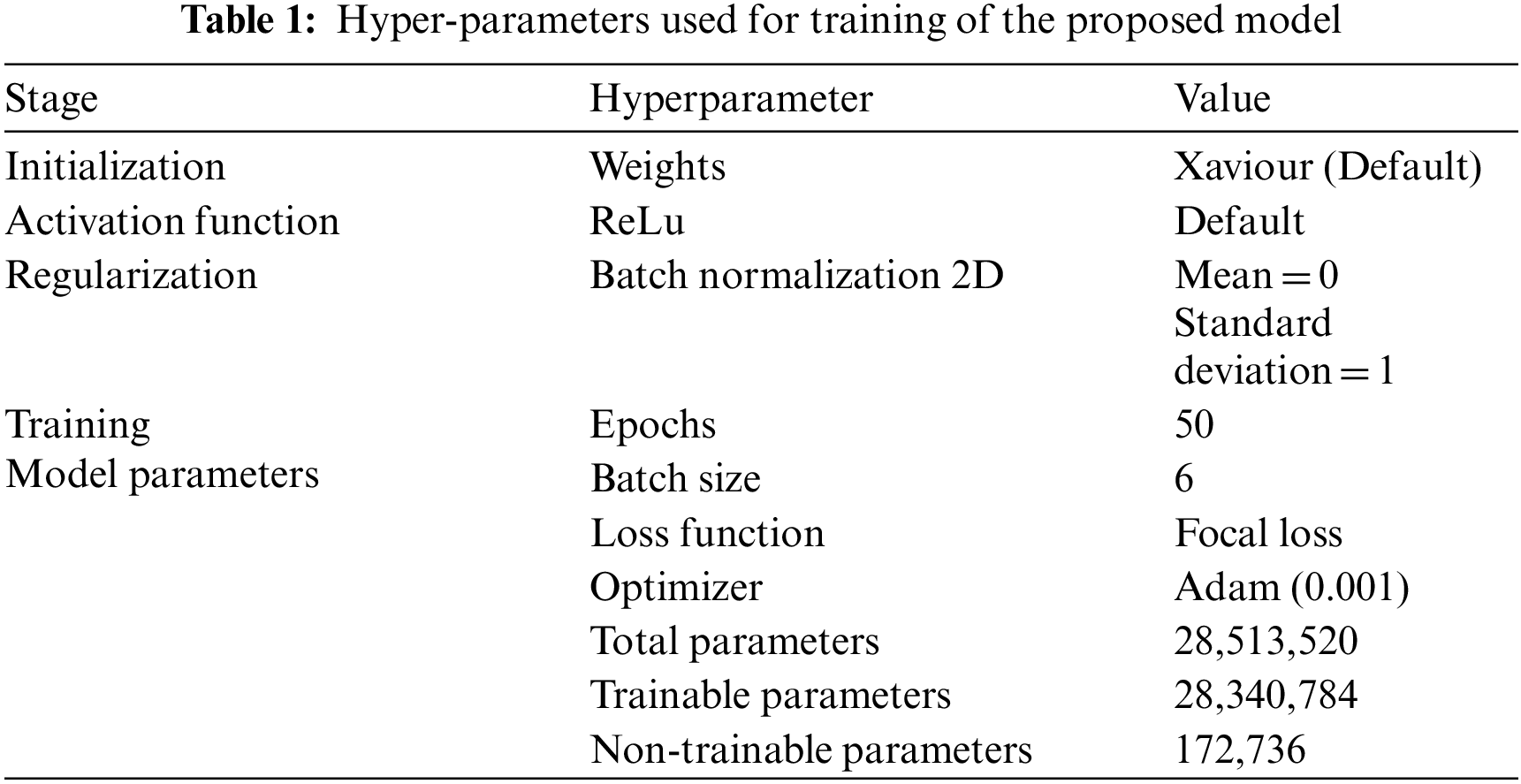
The Tab. 1 unveils the setting used for training of model training.
For evaluation of the proposed architecture, we have used these three performance measures named as DSC, sensitivity and HD. The DSC computes the similarity between the actual and predicted values.
Sensitivity is a measure that finds out how correctly it identifies the true positives from the predictions.
The HD is the longest distance you can be forced to travel by an opponent who chooses a point in one of the two sets and then forces you to travel to the other set. In other words, it is the longest distance between a point in one set and the nearest point in the other set.
5.2 Training and Testing Results
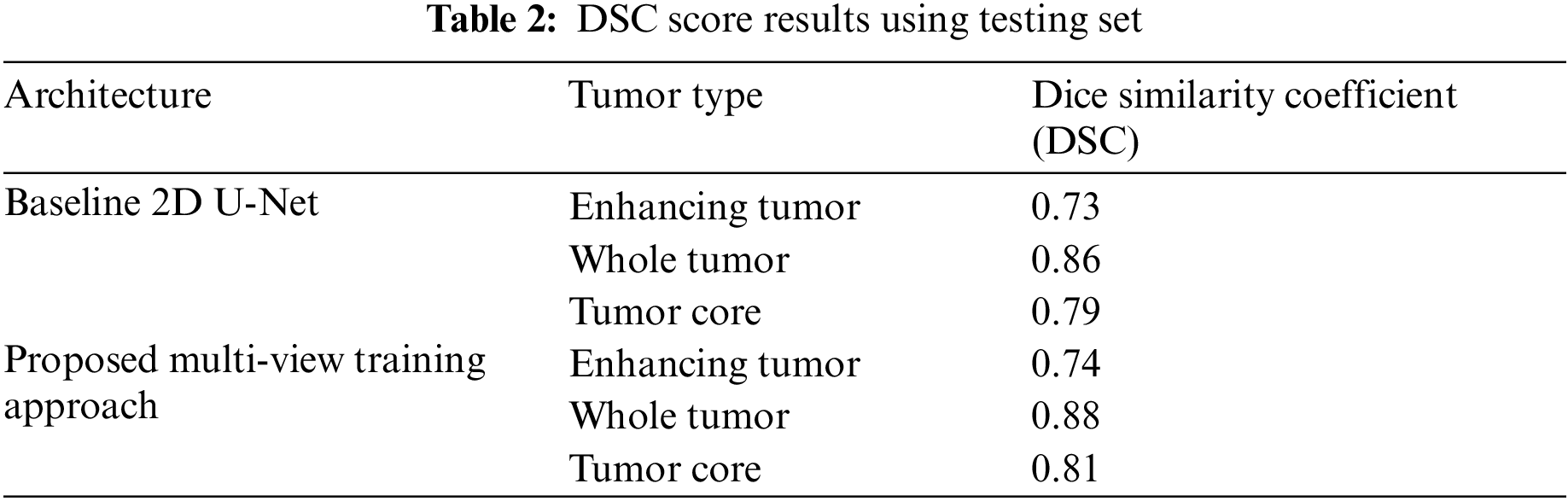
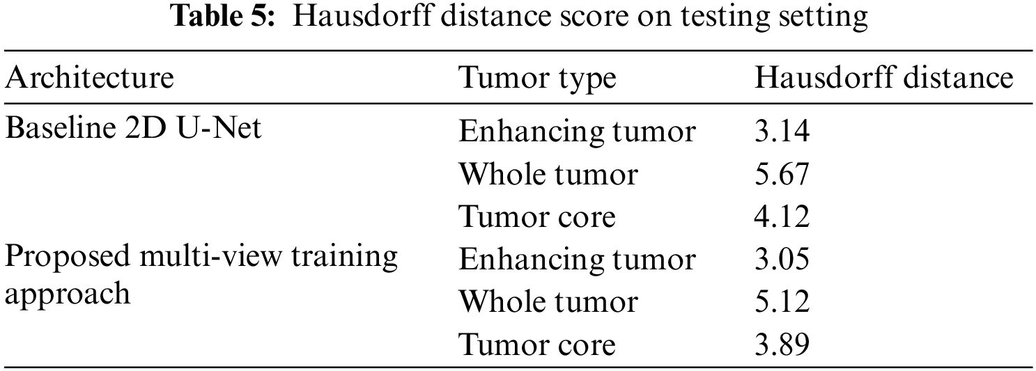
We have trained the proposed multi-view dataset on the standard U-Net architecture and compared it with training on single view to compare the effectiveness of the proposed approach. The results on four performance measures, DSC, sensitivity, specificity and HD is shown in Tabs. 2–5. The Tab. 2 shows the DSC score of ET, WT and TC comparison with baseline 2D U-Net architecture. The results show an improvement of 2% on ET, WT, and TC sub-tumor types using a multi-view training approach.
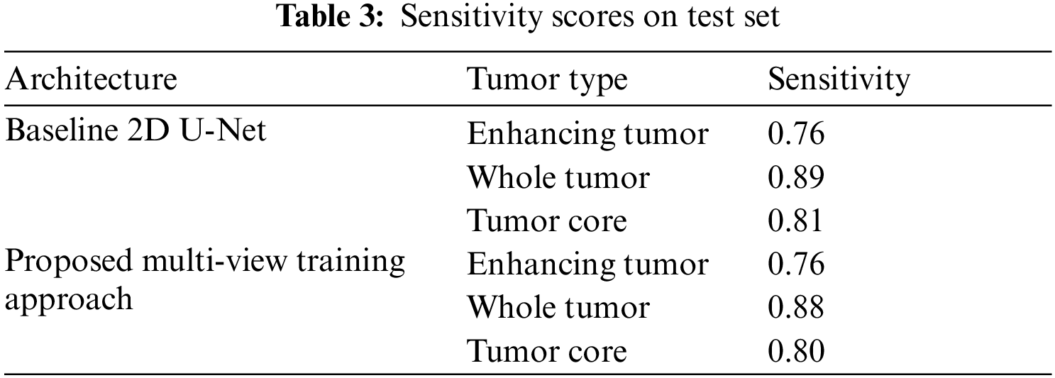

Similarly, the Tab. 3 shows the sensitivity scores of ET, WT and TC sub-tumor types. The comparison of sensitivity scores with baseline 2D U-Net is quite promising as the scores of WT and TC is better as compared to 2D U-Net due to capturing contextual information using multi-view approach.
The Tab. 4 shows the Specificity scores of sub-tumor types ET, WT and TC. The scores of specificity is similar to sensitivity.
The proposed multi-view approach helps to capture inter-slice information, and the combined approach outperforms the vanilla U-Net. The CRF post-processing technique also increases the performance and reduces the Hausdorff distance. This embedded post-processing approach reduces the outliers.
As far as the dataset is concerned, the BraTS Dataset consists of T1, T1-Contrast Enhanced (T1-CE), T2, and FLAIR are the four modalities used in the BraTs dataset for HGG and LGG volumes. Each MRI volume has a dimension of 155240240. Ground Truth (GT) labels for each patient segmentation include ET, Non-Enhancing Tumor (NET), and Peritumoral Edema (PE). The data set is comprised of 349 volumes (259 HGG and 76 LGG). The distribution of labels in the training and testing set is shown in Figs. 4–6 shows every separated label from a single patient slice.

Figure 4: Distribution of labels in training set

Figure 5: Distribution of labels in test set

Figure 6: Distribution of labels in test set
The visual results of segmented tumor regions on the validation set are shown in axial, sagittal, and coronal views with heat maps generated from intermediate CNN slides to assess results visually. The sub-tumor types are represented in different colors for proper evaluation. The Figs. 7–9 are from a slice from a sample patient. This overlapping fusion enables to capture of inter-slice information.

Figure 7: Heatmaps and tumor overlap on sample slice of patient in axial plane

Figure 8: Heatmaps and tumor overlap on sample slice of patient in coronal plane

Figure 9: Heatmaps and tumor overlap on sample slice of patient in saggitial plane
The visual results of different patients in different slices are shown in Figs. 10–13. The sub-tumor types are represented in different colors for proper evaluation.

Figure 10: Distribution of labels in test set

Figure 11: Distribution of labels in test set

Figure 12: Distribution of labels in test set

Figure 13: Distribution of labels in test set
In this study, we have proposed a novel multi-view training strategy for the brain tumor segmentation problem. Instead of combining multi-view model predictions, multi-view input is given to U-Net-based architecture, which achieved better results than U-Net-based architecture. Assessment of results shows the effectiveness of the proposed approach. In addition, the CRF reduced the false positives from the predictions and improved the segmentation results. This model has been applied to BraTS 2019 dataset, and cross-validation is performed to check the accuracy of results. The proposed approach achieves DSC of 0.77 on ET, 0.90 on WT, and 0.84 on TC with a reduced HD of 3.05 on ET, 5.12 on WT, and 3.89 on TC.
Funding Statement: This research was supported by Suranaree University of Technology, Thailand, Grant Number: BRO7-709-62-12-03.
Conflicts of Interest: The authors declare that they have no conflicts of interest to report regarding the present study.
1. D. Kharat, P. Kailash, K. Pradyumna and M. B. Nagori, “Brain tumor classification using neural network based methods,” International Journal of Computer Science and Informatics, vol. 2, no. 2, pp. 1075, 2012. [Google Scholar]
2. P. Kleihues and L. H. Sobin, “World health organization classification of tumors,” Cancer, vol. 88, no. 12, pp. 2887–2887, 2000. [Google Scholar]
3. L. Lüdemann, W. Grieger, R. Wurm, M. Budzisch, B. Hamm et al., “Comparison of dynamic contrast-enhanced MRI with WHO tumor grading for gliomas,” European Radiology, vol. 11, no. 7, pp. 1231–1241, 2001. [Google Scholar]
4. I. Ali, C. Direkog˘lu and S. Melike, “Review of MRI-based brain tumor image segmentation using deep learning methods,” Procedia Computer Science, vol. 102, pp. 317–324, 2016. [Google Scholar]
5. S. Abbasi and F. Tajeripour, “Detection of brain tumor in 3D MRI images using local binary patterns and histogram orientation gradient,” Neurocomputing, vol. 219, pp. 526–535, 2017. [Google Scholar]
6. G. R. Chandra and H. R. K. Ramchanda, “Tumor detection in brain using genetic algorithm,” Procedia Computer Science, vol. 79, pp. 449–457, 2016. [Google Scholar]
7. P. Mlynarski, H. Delingette, A. Criminisi and N. Ayache, “3D convolutional neural networks for tumor segmentation using long-range 2D context,” Computerized Medical Imaging and Graphics, vol. 73, pp. 60–72, 2019. [Google Scholar]
8. S. Pereira, A. Pinto, V. Alves and C. A. Silva, “Brain tumor segmentation using convolutional neural networks in MRI images,” IEEE Transactions on Medical Imaging, vol. 35, no. 5, pp. 1240–1251, 2016. [Google Scholar]
9. H. Chen, Z. Qin, Y. Ding, L. Tian and Q. Zhen, “Brain tumor segmentation with deep convolutional symmetric neural network,” Neurocomputing, vol. 392, pp. 305–313, 2020. [Google Scholar]
10. C. Chen, L. Xiaopeng, D. Meng, Z. Junfeng and L. Jiangyun, “3D dilated multi-fiber network for real-time brain tumor segmentation in MRI,” in Int. Conf. on Medical Image Computing and Computer-Assisted Intervention, Springer, Cham, 2019. [Google Scholar]
11. F. Isensee, P. Kickingereder, W. Wick, M. Bendszus and K. H. Maier-Hein, “No new-net,” in Int. MICCAI Brainlesion Workshop, Springer, Cham, 2018. [Google Scholar]
12. G. Chandra and K. Rao, “Tumor detection in brain using genetic algorithm,” Procedia Computer Science, vol. 79, pp. 449–457, 2016. [Google Scholar]
13. H. Mohsen, E. El-Dahshan, E. El-Horbaty and A. Salem, “Classification using deep learning neural networks for brain tumors,” Future Computing and Informatics Journal, vol. 3, no. 1, pp. 68–71, 2018. [Google Scholar]
14. E. Abdel-Maksoud, M. Elmogy and R. Al-Awadi, “Brain tumor segmentation based on a hybrid clustering technique,” Egyptian Informatics Journal, vol. 16, no. 1, pp. 71–81, 2015. [Google Scholar]
15. S. Abbasi and F. Tajeripour, “Detection of brain tumor in 3D MRI images using local binary patterns and histogram orientation gradient,” Neurocomputing, vol. 219, pp. 526–535, 2017. [Google Scholar]
16. S. Hussain, S. Anwar and M. Majid, “Segmentation of glioma tumors in brain using deep convolutional neural network,” Neurocomputing, vol. 282, pp. 248261, 2018. [Google Scholar]
17. U. E. Hani, S. Naz and I. A. Hameed, “Automated techniques for brain tumor segmentation and detection: A review study,” in 2017 Int. Conf. on Behavioral, Economic, Socio-cultural Computing (BESC), Krakow, Poland, pp. 1–6, 2017. [Google Scholar]
18. A. A. Khan, P. Uthansakul, P. Duangmanee and M. Uthansakul, “Energy efficient design of massive MIMO by considering the effects of nonlinear amplifiers,” Energies, vol. 11, pp. 1045, 2018. [Google Scholar]
19. P. Uthansakul and A. A. Khan, “Enhancing the energy efficiency of mmWave massive MIMO by modifying the RF circuit configuration,” Energies, vol. 12, pp. 4356, 2019. [Google Scholar]
20. P. Uthansakul and A. A. Khan, “On the energy efficiency of millimeter wave massive MIMO based on hybrid architecture,” Energies, vol. 12, pp. 2227, 2019. [Google Scholar]
21. A. A. Khan, P. Uthansakul and M. Uthansakul, “Energy efficient design of massive MIMO by incorporating with mutual coupling,” International Journal on Communication Antenna and Propagation, vol. 7, pp. 198–207, 2017. [Google Scholar]
22. L. Lüdemann, W. Grieger, R. Wurm, M. Budzisch, B. Hamm et al., “Comparison of dynamic contrast-enhanced MRI with WHO tumor grading for gliomas,” European Radiology, vol. 11, no. 7, pp. 1231–1241, 2001. [Google Scholar]
 | This work is licensed under a Creative Commons Attribution 4.0 International License, which permits unrestricted use, distribution, and reproduction in any medium, provided the original work is properly cited. |