DOI:10.32604/cmc.2022.024642
| Computers, Materials & Continua DOI:10.32604/cmc.2022.024642 | |
| Article |
Mean Opinion Score Estimation for Mobile Broadband Networks Using Bayesian Networks
1College of Engineering, A'Sharqiyah University (ASU), Ibra, 400, Oman
2Communication Systems and Networks Research Lab, Malaysia-Japan International Institute of Technology, Universiti Teknologi Malaysia, Kuala Lumpur, 54100, Malaysia
3Department of Electronics and Communication Engineering, Faculty of Electrical and Electronics Engineering, Istanbul Technical University (ITU), Istanbul, 34467, Turkey
4Advanced Informatics Department, Razak Faculty of Technology and Informatics, Universiti Teknologi Malaysia, Kuala Lumpur, 54100, Malaysia
*Corresponding Author: Abdulraqeb Alhammadi. Email: abdulraqeb.alhammadi@utm.my
Received: 25 October 2021; Accepted: 25 January 2022
Abstract: Mobile broadband (MBB) networks are expanding rapidly to deliver higher data speeds. The fifth-generation cellular network promises enhanced-MBB with high-speed data rates, low power connectivity, and ultra-low latency video streaming. However, existing cellular networks are unable to perform well due to high latency and low bandwidth, which degrades the performance of various applications. As a result, monitoring and evaluation of the performance of these network-supported services is critical. Mobile network providers optimize and monitor their network performance to ensure the highest quality of service to their end-users. This paper proposes a Bayesian model to estimate the minimum opinion score (MOS) of video streaming services for any particular cellular network. The MOS is the most commonly used metric to assess the quality of experience. The proposed Bayesian model consists of several input data, namely, round-trip time, stalling load, and bite rates. It was examined and evaluated using several test data sizes with various performance metrics. Simulation results show the proposed Bayesian network achieved higher accuracy overall test data sizes than a neural network. The proposed Bayesian network obtained a remarkable overall accuracy of 90.36% and outperformed the neural network.
Keywords: Quality of experience; quality of service; bayesian networks; minimum opinion score; artificial intelligence; prediction; mobile broadband
As support for high-speed internet access, mobile broadband (MBB) networks have grown very quickly. Data demand has risen rapidly because of the large number of users using various mobile technology and Internet services to access data. Hence, to enhance the quality of service, it is highly necessary to monitor network performance. Performance and quality assessment are becoming increasingly critical for mobile network operators with the rising demand on current networks. The current fourth-generation (4G) networks are insufficient for bandwidth-hungry and low latency applications. Enhanced MBB (eMBB) is the first of the three main categories in fifth-generation (5G), extending to existing 4G networks. The 5G eMBB offers high-speed data, low latency video streaming, and seamless mobility. Video streaming is the most used service by subscription users. It plays the main role in evolving the quality of services (QoS) and user experience for the MBB providers. Thus, monitoring network performance is very important to guarantee users satisfaction. Different network infrastructures support various video services. For example, video over Internet protocol (also known as AV-over-IP) is a technology that delivers video service over a conventional cable network infrastructure. In contrast, video over LTE (ViLTE) is an enhanced technology that supports voice services with a high-quality video channel over LTE network infrastructure. These services are improved continuously by mobile service providers to increase the number of satisfied users in cellular networks.
International telecommunication union (ITU) introduced a new term called mean opinion score (MOS), which assesses mobile network providers by evaluating the end-users’ satisfaction by obtaining users opinions of a network's performance [1]. The MOS metric is widely used for several services and applications such as audio, audiovisual, and video. These services have various methods to assist in scoring their service quality [2]. It also includes entertainment services such as conversational, audiovisual, listening, talking, and video. Several MOS levels have been defined in ITU-T P.800.1, which can be categorized into five levels based on the network quality [2]. Various methodologies have also been used to examine network services, including audio, audiovisual, and video. While the use of “reference quality indicator” and its general acceptance has an obvious advantage, MOS is frequently used without enough assessment of its scope or limits. In [3], the common issues with various types of MOS are highlighted and a variety of alternative methods for media quality measurement are discussed. Numerous works have investigated and evaluated various types of service over wireless networks. In [4], the authors evaluated the perceived quality of the ViLTE service by performing an experimental testbed realized at a mobile provider. Several network QoS parameters such as packet loss and packet delay variation are utilized to predict differential MOS of the ViLTE services. In [5], the authors proposed a prediction model based on data collected from 3G and 4G networks to estimate the quality of experience (QoE) of web browsing and voice services. The model aimed to estimate the MOS scale based on the user-perceived web and video qualities. In [6], a simplified E-model based on a subjective MOS prediction model is proposed. This model aimed to enhance the objective measurement tool for specific codecs. In [7], random neural networks are utilized to objectively predict video quality, consisting of a three-layer feed-forward with a gradient descent training algorithm. The predicted MOS achieved accuracy with approximately 50% compared to other models. However, most proposed models deal with voice and web browsing services that are insufficient to evaluate the network performance. Video streaming and data become very important in people's daily life than voice because of the increase in smartphone video applications that require more mobile video traffic. Thus, more studies are required to evaluate video streaming performance over various MBB networks. Several optimization techniques, such as artificial intelligence (AI) can be used to assist mobile services providers to monitor and optimize their network performance. Currently, AI has become very popular and involved in many different technologies. It is considered one of the most promising solutions in the 5G networks that have been used to mimic human intelligence to support and improve a wide variety of applications. Bayesian networks are a combination of AI and several theories, such as a graph, decision, and probability that uses Bayesian inference for probability computations. Bayesian inference is used in many studies such as [8,9] that help to infer missing or unknown data.
In this paper, we propose a Bayesian graphical model to evaluate MBB network performance by estimating the MOS from a dataset. The quality of video streaming service is considered, which depends on several parameters such as stalling time, end-to-end latency, downlink bite rate. The estimated MOS indicates service quality users’ satisfaction, which helps mobile network operators maintain their network quality to satisfy users’ requirements. The remainder of this paper is organized as follows. Section 2 provides a background on quality models used to determine services and applications’ performance. Section 3 explains in detail the proposed Bayesian graphical model and procedure and performance metrics. Section 4 analyses and evaluates the performance of the proposed model. Section 5 concludes the paper.
In this section, the background on the quality models and Bayesian networks are discussed. In the quality models, we present various quality models to determine or estimate a network performance based on the end-users preceptive. In the Bayesian networks, we introduce usage Bayesian networks through an experimental perspective on probabilistic reasoning to predict an unknown particulate variable.
Numerous services and applications, such as video streaming and real-time gaming suffer from buffering, dropped frames, and additional delay because of end-to-end transmission and video encoding and decoding. Moreover, some network constraints, such as limited bandwidth, network congestion, and packet loss can negatively affect the end user's QoE. Thus, several strategies for resource and network management are required to optimize user satisfaction. Various system configurations should consider the subjective user ratings to optimize the network performance.
ITU provides a recommendation of various quality models to determine or estimate network performance based on the end-users’ preceptive. This recommendation specifies the terminologies to be used in conjunction with quality expressions of audio, audiovisual, and video in terms of MOS. Several identifiers are used to observe the MOS rate for quality of video (VMOS) service provided by mobile operators, such as the subjective, objective, and estimated, which are referred to as S-VMOS, O-VMOS, and E-VMOS, respectively [2]. In addition, various factors also influence the VMOS value application, viewing device display size, and display resolution [ITU-T P.800.2]. The S-VMOS refers to subjective video quality. It is based on the collected VMOS value laboratory test where it is determined by the arithmetic mean value of subjective judgments. Subjective tests were carried out according to obtain results in terms of MOS-VQS [10,11]. O-VMOS refers to the objective video quality that depends on an algorithmic quality real-time evaluation model for determining the MOS score. The real-time evaluation model utilizes various real-time objective metrics obtained from information carried in the video streams and corresponding networks. ITU presented several models to investigate bitstream assessment of video media streaming quality [12,13].
E-VMOS refers to the estimated video quality calculated by a network planning model. It aims to predict video quality over a network in non-real-time parameters. The E-VMOS is used mostly where the MOS values are not determined in real-time models. Some non-real-time models have been defined in [14,15]. Fig. 1 shows the relationship between VMOS identifiers. For the subjective model, the real-time parameters that come from the system feed the subjective test directly to determine the S-VMOS. In the objective model, the value of S-VMOS depends on several factors, such as real-time video streams and system and calibration from the subjective test. However, in E-VMOS, video test library and non-real-time parameters feed the network planning model to predict the value of E-VMOS. However, these methods present a general concept of MOS models for various services. The S-VMOS and O-VMOS are required for real-time parameters, which lead to complicated processes and high costs, whereas E-VMOS requires only a sufficient database that can be collected at a specific time in the desired area for testing the network performance.

Figure 1: Relationship between VMOS identifiers [2]
Bayesian networks are the method of choice for explainable reasoning in AI. This work aims to introduce a prediction model based on Bayesian networks through an experimental perspective on probabilistic reasoning. Bayesian networks are probabilistic graphical models that represent joint probability distributions of a set of random variables. The networks measure the conditional dependence structure of these variables according to Bayes theorem:
where P(A|B) represents the posterior probability of an event A given prior knowledge of a condition B. P(B|A) is a conditional probability of event B given prior knowledge of a condition A.
The graphical model of the Bayesian network consists of several nodes N (also known as vertices)

Figure 2: Basic concept of the bayesian graphical model
Priors P(Y) and conditionals P(Xi|Y) for Naïve Bayes where it can be defined as a joint distribution:
Bayesian network is a type of network that contains data on the causal probability correlations between variables and is frequently used to help in decision making. The Bayes theorem usually updates the causal probability, where the Bayesian nodes indicate the inter-variable dependency structure and the conditional relationships depict the directed arcs in the form of a directed acyclic graph.
The conditional probabilities of p(z) represented by directed acyclic graph can be mathematically expressed as follows:
The conditional probability of p(z) represents the query stored in the graphical network in Fig. 3. Eq. (5) can be written efficiently in terms of summation into four separate summations, one over each variable. It requires enumerating all possible combinations of assignments to X, Y, H, and F, and then multiplying the factors for each node.

Figure 3: Directed acyclic graph
The variable elimination on Fig. 3 and Eq. (5) uses elimination order X, Y, H, F. The variable F can be eliminated by gathering the similar variable F (in this case
Similarly, the next variable H also can be eliminated because it has a similar term that can be computed in terms of factor
Finally, the probability of variable Z is simplified as presented in Eq. (7) over variables X and Y.
3 Proposed Model and Performance Metrics
This section presents the proposed Bayesian graphical model, which consists of several nodes and directed edges. This study is an extension of our previous work presented in [16]. The proposed model aims to estimate the MOS of video services provided by MBB networks. The estimation process of video quality requires non-real-time parameters which can be obtained from data measurements. Fig. 4 illustrates the proposed model, which comprises seven primary nodes. Three input data nodes, namely, stalling load,

Figure 4: Proposed bayesian network model for estimating MOS
Bayesian inference using the Gibbs Sampler (OpenBUGS) is a visual tool used to develop various graphical models [18]. It is an open-source software that assists in designing and simulating different Bayesian graphical models. The proposed model was built by utilizing the features of OpenBUGS, which estimate the probability distribution of unknown node-based Gibbs sampler. First three nodes
where
where
The initial values (
Then, the Bayesian model follows the Bayes’ theorem to infer unknown nodes, which generates a posterior probability distribution based on the prior probability distribution and the likelihood function of the data. Thus, the conditional probability of the posterior distribution is given by the product of the prior and likelihood function.
The framework of the proposed prediction model treated in this work is illustrated in Fig. 5. The framework consists of two main stages: real-time objective MOS and non-real-time estimated MOS. The former refers to the raw database collected from different mobile operators where the MOS is determined by an algorithmic quality real-time evaluation model. Meanwhile, the latter utilizes the input video parameters to estimate the MOS over a non-real-time network. These input parameters are considered necessary in QoE and QoS planning; thus, they feed the proposed Bayesian model to predict the MOS values.

Figure 5: A general framework of estimated MOS process
The sampling distribution is based on the Gibbs sampler, which is one of the Markov chain Monte Carlo (MCMC) algorithms. The Gibbs sampling algorithm was employed to draw samples from the high dimensional joint distribution [19]. It draws a large number of samples denoted with
Next loop through the following steps:
These steps are repeated continuously with generated values to replace the initial values that burn the sample at the first loop. The chain of values produced by these procedures refers to the Markov chain (MC), which is a joint posterior distribution that converges to its equilibrium distribution.
In this section, the performance of the proposed model is evaluated based on an unknown estimated MOS (EMOS) node. The OpenBUGS tool is the most widely used software packages for fitting Bayesian models because it enables the user to specify a Bayesian model (prior and likelihood) in the R language. In this sense, this software was utilized to evaluate and analyze the proposed model based on MCMC simulations following Bayesian statistical theory. The specification of the proposed model targets a posterior distribution to infer the unknown values. OpenBUGS provides and displays the numeric results of the estimation of the unknown MOS nodes and a summary of the posterior inference.
The EMOS was examined using different testing methods. The testing data were divided into four test groups: 20%, 40%, 60%, and 80%. Each testing data were examined separately to investigate the effectiveness of the testing data size. All tested data sizes used the same parameters during the inference phase. The proposed model was initialized, updated with 1000 iterations for burning-in samples, and then updated with 10000 iterations for estimating the EMOS node. Burning-in samples were used to discard the effect of initially generated samples on the posterior inference. The estimated EMOS node is represented by a value within a range of 1 to 5. These values indicate network quality and user satisfaction. Fig. 6 shows the different qualities and the lowest MOS Score limit for each one. The limit values are from the ITU-T G.107 standards [20]. Each range in the MOS scale indicates the network quality and user satisfaction. Several performance metrics were used to compare the difference between the actual AMOS and the EMOS values. In this work, four performance metrics were used: mean absolute error (MAE), mean squared error (MSE), mean percentage error (MPE), and mean squared error (RMSE) which can be given as follows:
where AMOS and EMOS are actual and estimated MOS, respectively. n represents the number of test data. Eq. (15) was used to calculate the error rate and feasibility of the proposed model. Finally, the proposed Bayesian model is compared with a neural network in terms of accuracy.
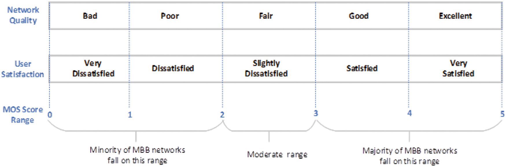
Figure 6: Relation between network quality and MOS value
In this section, the simulation results of the proposed model are presented and discussed. The test data are the same for the four cases to ensure a fair comparison. Fig. 7 shows an example of generated samples of a single MOS value of 3.5 during the sampling process for different iteration numbers. Most generated samples are bound between 3 and 4, considering the relative values to the actual MOS for all iterations. Increasing the number of iterations may result in a slight increase in system accuracy in such cases. Fig. 8 shows the dynamic tracing of generated values against iteration number for six estimated EMOS values during the inference process. These tracing figures analyze the pattern of the posterior distribution for obtaining estimated EMOS nodes. The results were obtained by running the MC chain for 10000 iterations with another 1000 iterations for the burn-in samples. Tab. 1 shows a statistical summary of the estimated EMOS nodes with present MC error. The MC represents the error margin when the MCMC samples were used to estimate the posterior mean. The table shows that the MC error achieved very low values for all EMOS nodes.

Figure 7: Generated samples of EMOS value (a) 2000 iterations (b) 5000 iterations (c) 10000 iterations
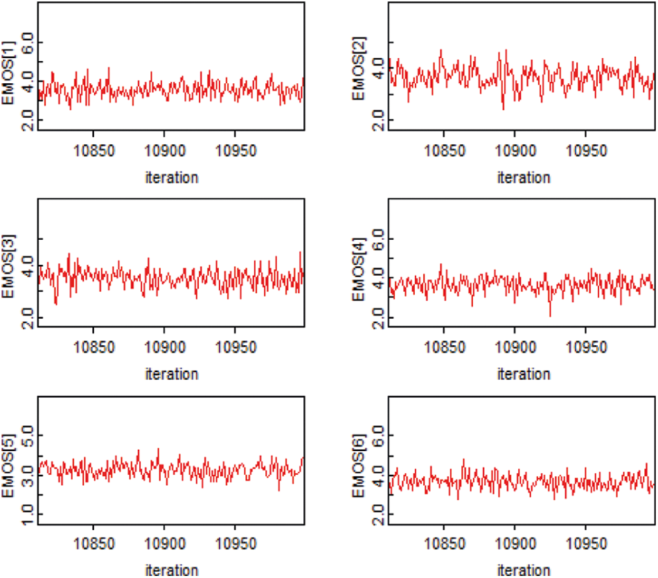
Figure 8: Dynamic tracing of six EMOS nodes

Fig. 9 shows the smoothed kernel density of six estimated MOS values. This figure is similar to a smoothed histogram where each iteration is distributed around the estimated node using a Kernel function, such as normal distributions instead of counting the estimates into bins of particular widths. The kernel density estimation is a means of estimating the posterior probability density function of a random variable. The high density concentrates between 3 and 4, which are the most accurate values of actual MOS. Bell-shaped posterior distributions indicate that the MC chain has reached the convergence level.
Fig. 10 visualizes the various plotting types of estimated MOS values over several points of data. Fig. 10a shows the boxplot of the posterior distributions of all estimated MOS values were summarized side by side. The interquartile range and anticipated mean value of MOS are represented by the green boxes and the center lines, respectively. The box arms extend to cover the center 95% of the distribution, with their ends corresponding to the 2.5% and 97.5% quantiles. More informative statistics and visualizations are provided in Fig. 10b, which depicts the full posterior distribution through shading, with the strip blackness at each data point defined as proportionate to the estimated density. Similarly, Fig. 10c represents the “caterpillar” plot, which is conceptually very similar to Fig. 10a. The x-axis for each distribution is summarized by a horizontal line representing the 95% interval, whereas the dots indicate the mean location.

Figure 9: Kernel density of six EMOS nodes

Figure 10: Visualization of estimated MOS (a) Boxplot (b) Caterpillar (c) Density strip
Fig. 11 shows a bar graph of AMOS, EMOS with absolute and squared error against random testing points. The absolute error of estimating MOS with AMOS of greater than 3 is lower compared to the MOS smaller than 3 because the data contain MOS greater than 3, and the majority of MBB networks fall in this score with a good and satisfying network. Thus, the model trains well with these MOS compared with the small data of MOS = 1. The maximum absolute average errors for MOS greater and smaller than 3 are 0.20 and 0.45, respectively.

Figure 11: Graph bar of AMOS, EMOS with absolute and squared error against random test points
Fig. 12 illustrates the comparison between the proposed Bayesian and neural networks in terms of MAE, MSE, and RMSE over test data sizes. In this comparison, these test data sizes are considered (20%, 40%, and 60%) where a higher test data size cannot be implemented practically. The dataset is divided into 20% test data and 80% training data in most common works. However, the proposed model is examined for two more test data sizes. The figure shows that the MAE, MSE, and RMSE increase when the size of test data increases. In the Bayesian network, the test data size of 20% achieved the lowest MAE and MSE of 0.148 and 0.025, respectively, whereas the test data size of 60% achieved the highest MAE and MSE of 0.259 and 0.110, respectively. Similarly, in the neural network, the test data size of 20% achieved the lowest MAE and MSE of 0.21 and 0.10, respectively, whereas the test data size of 60% achieved the highest MAE and MSE of 0.68 and 1.21, respectively. The results are because when the test data size is large, the training data will be small, which is insufficient to train the model. Thus, the estimated nodes have greater variance with less training data, while the performance statistic will have greater variance with less testing data. The proposed Bayesian network outperforms the neural network in all test data sizes. Tab. 2 summarizes different performance metrics over test data sizes.

Figure 12: Comparison between bayesian and neural networks over test data sizes

Fig. 13 demonstrates the accuracy comparison between the Bayesian and neural networks. The proposed Bayesian network achieved a high accuracy of 95.72%, 93.87%, and 81.49% for the test data sizes of 20%, 40%, and 60%, respectively. The neural network achieved a low accuracy of 88.07%, 81.00%, and 35.42% for test data size of 20%, 40%, and 60%, respectively. Both networks obtained the highest accuracies when using 20% of the test data size. However, the neural network had poor accuracy of 35.42% when using 60% of the test data size compared with the Bayesian network. Overall, the Bayesian and neural networks achieve 90.36% and 68.16%, respectively. Therefore, the proposed Bayesian network achieved remarkable accuracy and outperformed the neural network.
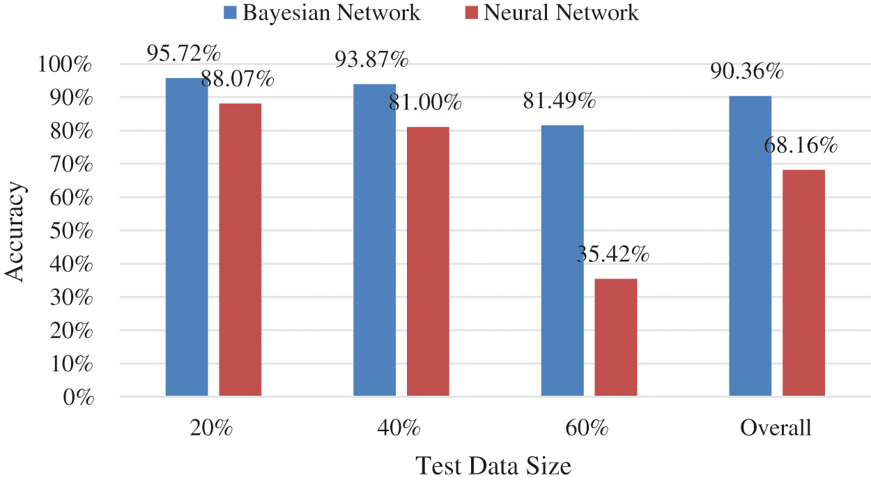
Figure 13: Accuracy comparison between bayesian and neural networks
In the present work, a Bayesian network based on a probabilistic graphical model to estimate MOS in MBB networks is proposed. Video streaming data have been utilized for training and testing the proposed model to estimate accurate MOS. Several performance metrics have been used to evaluate the proposed model with various implementing scenarios. The results showed that the proposed Bayesian network achieved high accuracy overall test data size compared with the neural network. Overall, the Bayesian network obtained an accuracy of 90.36% overall test data sizes. Therefore, the proposed Bayesian network achieved remarkable accuracy and outperformed the neural network. An interesting path for future investigation would be to explore the MOS of several services, such as video streaming with multiple resolutions, gaming, and web browsing. Multiple databases of several mobile network providers can be also be investigated further.
Acknowledgement: This research study was sponsored by the Universiti Teknologi Malaysia through the Professional Development Research University Grant (No. 05E92). It is also funded using the Collaborative Research Grant National (Grant reference PY/2019/02791).
Funding Statement: The research leading to these results has received funding from The Research Council (TRC) of the Sultanate of Oman under the Block Funding Program with Agreement No. TRC/BFP/ASU/01/2019.
Conflicts of Interest: The authors declare that they have no conflicts of interest to report regarding the present study.
1. ITU, “Series P: Telephone transmission quality, telephone installations, local line networks, vocabulary for performance, quality of service and quality of experience. T P.10/G.100,” in International Telecommunication Union Telecommunication Standardization Sector, Geneva, Switzerland: International Telecommunication Union (ITU2017. [Google Scholar]
2. ITU, “Series P: Terminals and subjective and objective assessment methods: Methods for objective and subjective assessment of speech and video quality: Mean opinion score (MOS) terminology, ITU-T Rec. P.800.1,” in Telecommunication Standardization Sector ITU, Geneva, Switzerland: International Telecommunication Union (ITU2016. [Google Scholar]
3. R. C. Streijl, S. Winkler and D. S. Hands, “Mean opinion score (MOS) revisited: Methods and applications, limitations and alternatives,” Multimedia Systems, vol. 22, pp. 213–227, 2016. [Google Scholar]
4. C. Callegari, R. G. Garroppo, S. Giordano, C. C. Labrozzo, G. Procissi et al., “Experimental analysis of ViLTE service,” IEEE Access, vol. 6, pp. 21129–21139, 2018. [Google Scholar]
5. V. Pedras, M. Sousa, P. Vieira, M. P. Queluz, A. Rodrigues et al., “A no-reference user-centric QoE model for voice and web browsing based on 3G/4G radio measurements,” in 2018 IEEE Wireless Communications and Networking Conf. (WCNC), Barcelona, Spain, pp. 1–6, 2018. [Google Scholar]
6. T. Daengsi and P. Wuttidittachotti, “QoE modeling for voice over ip: Simplified e-model enhancement utilizing the subjective MOS prediction model: A case of G. 729 and Thai users,” Journal of Network and Systems Management, vol. 27, pp. 837–859, 2019. [Google Scholar]
7. T. Ghalut and H. Larijani, “Non-intrusive method for video quality prediction over lte using random neural networks (rnn),” in 2014 9th Int. Symp. on Communication Systems, Networks & Digital Sign (CSNDSP), Manchester, UK, pp. 519–524, 2014. [Google Scholar]
8. Y. Zang, T. Hu, T. Zhou and W. Deng, “An automated penetration semantic knowledge mining algorithm based on bayesian inference,” Computers, Materials & Continua, vol. 66, pp. 2573–2585, 2021. [Google Scholar]
9. A. -I. Al-Omari, A. -S. Hassan, H. -F. Nagy, A. -R. -A. Al-Anzi, L. Alzoubi et al., “Entropy bayesian analysis for the generalized inverse exponential distribution based on URRSS,” Computers, Materials & Continua, vol. 69, pp. 3795–3811, 2021. [Google Scholar]
10. ITU, “P.912 subjective video quality assessment methods for recognition tasks,” in Int. Telecommunications Union Telecommunication Sector, Geneva, Switzerland: International Telecommunication Union (ITUpp. 72400Z, 2016. [Google Scholar]
11. ITU, “913, Methods for the subjective assessment of video quality, audio quality and audiovisual quality of internet video and distribution quality television in any environment,” in International Telecommunication Union, Geneva, Switzerland: International Telecommunication Union (ITU2021. [Google Scholar]
12. ITU, “P.1202. Parametric non-intrusive bitstream assessment of video media streaming quality,” in International Telecommunications Union Telecommunication Sector, Geneva, Switzerland: International TelecommunicationUnion (ITU2013. [Google Scholar]
13. ITU, “J.343: Hybrid perceptual bitstream models for objective video quality measurements,” in International Telecommunications Union Telecommunication Sector, Geneva, Switzerland: International Telecommunication Union (ITU2014. [Google Scholar]
14. T. ITU, “1070 multimedia quality of service and performance–generic and user-related aspects,” in Opinion Model for Video Telephony Applications, Geneva, Switzerland: International Telecommunication Union (ITU2012. [Google Scholar]
15. ITU-T, “G.1071: Opinion model for network planning of video and audio streaming applications,” in International Telecommunications Union Telecommunication Sector, Geneva, Switzerland: International Telecommunication Union (ITU2016. [Google Scholar]
16. A. Alhammadi, A. El-Saleh, and I. Shayea, “MOS prediction for mobile broadband networks using Bayesian artificial intelligence,” in 2021 Int. Conf. on Artificial Intelligence and Computer Science Technology (ICAICST), Yogyakarta, Indonesia, pp. 47–50, 2021. [Google Scholar]
17. I. Shayea, M. Ergen, M. H. Azmi, D. Nandi, A. A. El-Salah et al., “Performance analysis of mobile broadband networks with 5G trends and beyond: Rural areas scope in Malaysia,” IEEE Access, vol. 8, pp. 65211–65229, 2020. [Google Scholar]
18. OpenBUGS (Access: 31-05-2021). “Bayesian inference using gibbs sampling,” [Online]. Available: https://www.openbugs.net/w/FrontPage. [Google Scholar]
19. A. E. Gelfand and A. F. Smith, “Sampling-based approaches to calculating marginal densities,” Journal of the American Statistical Association, vol. 85, pp. 398–409, 1990. [Google Scholar]
20. ITU-T, “ITU-T recommendation G. 107: The E-model, a computational model for use in transmission planning,” in Series G: Transmission Systems and Media, Digital Systems and Networks, Geneva, Switzerland: International Telecommunication Union (ITU2015. [Google Scholar]
 | This work is licensed under a Creative Commons Attribution 4.0 International License, which permits unrestricted use, distribution, and reproduction in any medium, provided the original work is properly cited. |