DOI:10.32604/cmc.2022.024762
| Computers, Materials & Continua DOI:10.32604/cmc.2022.024762 | |
| Article |
Simulation and Modelling of Water Injection for Reservoir Pressure Maintenance
1Department of Physics, University of Petroleum & Energy Studies, Dehradun 248007, Uttarakhand, India
2Department of Computer Science, University of Petroleum & Energy Studies, Dehradun 248007, Uttarakhand, India
3College of Computing and Informatics, Saudi Electronic University, Riyadh 11673, Saudi Arabia
4Department of Information Systems, College of Computer Science and Information Technology, King Faisal University, Al Hasa 36362, Saudi Arabia
*Corresponding Author: Md Ezaz Ahmed. Email: m.ezaz@seu.edu.sa
Received: 30 October 2021; Accepted: 01 March 2022
Abstract: Water injection has shown to be one of the most successful, efficient, and cost-effective reservoir management strategies. By re-injecting treated and filtered water into reservoirs, this approach can help maintain reservoir pressure, increase hydrocarbon output, and reduce the environmental effect. The goal of this project is to create a water injection model utilizing Eclipse reservoir simulation software to better understand water injection methods for reservoir pressure maintenance. A basic reservoir model is utilized in this investigation. For simulation designs, the reservoir length, breadth, and thickness may be changed to different levels. The water-oil contact was discovered at 7000 feet, and the reservoir pressure was recorded at 3000 pounds per square inch at a depth of 6900 feet. The aquifer chosen was of the Fetkovich type and was linked to the reservoir in the j+ direction. The porosity was estimated to be varied, ranging from 9% to 16%. The residual oil saturation was set to 25% and the irreducible water saturation was set at 20%. The vertical permeability was set at 50 md as a constant. Pressure Volume Temperature (PVT) data was used to estimate the gas and water characteristics.
Keywords: Eclipse; water injection; reservoir; modeling; simulation; oil saturation
Reservoir pressure maintenance by water injection is a procedure when water is injected into the oil-bearing reservoir to maintain its natural drive and improve recovery and production of oil and gas [1]. Water injection into the reservoir is used where reservoir conditions are not sufficient to achieve higher recoveries, primarily in reservoirs with solution gas drive. For over three decades water injection has been applied as a secondary method to enhance oil and gas recoveries particularly in the Croatian production fields Beničanci, Šandrovac, Lipovljani, Jamaica, Kozarice, Ivani6, and Utica, while in other fields the produced water is deposited into selected geologically suitable reservoirs. A long list of fields in the Middle East is receiving some sort of pressure maintenance. In Saudi Arabia, water injection is the major pressure-maintenance technique, although some gas also is being injected. In Iran, several smaller projects are underway to inject water for pressure maintenance. Though individual projects naturally vary somewhat in detail due to reservoir conditions and other factors, several threads are common to many of the water-injection projects in the area. With increasing frequency, the need for water injection is being considered immediately after results of the discovery well analyses are available. Early planning and the early installation of injection facilities are part of a philosophy in the area that is aimed at doing everything possible to ensure maximum recovery. Most water injection programs are aimed at maintaining an active water drive and reservoir pressure, although some additional reservoir sweep also is expected. It is no surprise that volumes are large. For example- in Saudi Arabia. Aramco was injecting over 12 million barrel per day (BPD) in 11 fields at the end of last year.
Water injection boosts the percentage (also known as the recovery factor) and extends the life of a reservoir’s production rate. Baker and his coworkers as described by al, low-salinity water flooding is used to boost oil recovery and sustain reservoir pressure. The permeability sandstone core plugs used are two different types. The findings of this study show that water devoid of free ions and modified low salinity water improved oil recovery more than formation water and saltwater as a secondary oil process. Liu et al. describe a geo-mechanical model for increasing oil recovery by water injection [2]. He et al. proposes a novel technique for improving oil recovery from unconventional oil reservoirs by combining synchronous inter-fracture injection and production (SiFIP) and asynchronous inter-fracture injection and production (AiFIP) technologies (AiFIP) [3]. The suggested techniques increase flooding performance by converting fluid injection between wells to hydraulic fractures from the same multi-fractured horizontal well (MFHW), which is a viable unconventional oil reservoir Enhanced Oil Recovery (EOR) technology.
The suggested EOR technique (AiFIP-CO2) has the potential to increase oil recovery while reducing CO2 emissions and water waste. The experiment is carried out by Liu et al. to solve the problem of fast rise in water content and loss of output in fault-block reservoirs during floods [4]. The findings revealed that while there was no direct link between oxygen consumption and crude oil viscosity, there was a water saturation tipping point. The temperature of the reaction affects the pace of the reaction.
Gideon Dordzie offers EOR reports in Feed Conversion Ratio (FCRs) and investigate the elements that impact the outcomes. Depending on the existence of formation damage, fines migration has been shown to either increase or impede EOR [5]. Farajzadeh et al. studied the chemical-based oil recovery. The characteristics of CO2-brine-oil systems, as well as the technique for injecting carbonated water, are investigated in the study. The dissolved CO2 can move into the oil phase, causing oil swelling and increasing oil mobility, which both increase sweep efficiency [6]. Mahmoudpour et al. employ Nano fluid hybrid injection to improve oil recovery in carbonate deposits [7]. Esene et al. investigate Carbonated Water Injection (CWI) in depth, focusing on key features such as displacement processes and recovery performance under various properties [8].
Sohrabi et al. evaluate the performance of CWI under reservoir settings, as well as the factors that influence the amount of oil recovered by CWI and its underlying processes using the CWI Joint Industry Project (JIP) [9]. The findings demonstrate that carbonated water-crude oil interactions at the pore size are quite distinct from the well-known processes found in conventional CO2 floods.
Low Salinity Surfactant Flooding (LSSF), according to, Hosseini et al., is a hybrid technique that incorporates all of the late benefits (wettability modification and interfacial tension reduction) of both low salinity water (LSW) and surfactant flooding [10]. Software has been investigated as a valuable tool for simulation and optimization, as well as innovative cost-effective and accurate application approaches. Donaldson et al. look at a variety of approaches and tactics for increasing oil recovery [11]. The influence of silicon oxide nanoparticles on the change in wettability of glass micromodels was studied using both experimental and computational modelling techniques, according to the researchers Rostami et al. [12]. Both the original water-wet and imposed oil-wet glass micromodels (aged in stearic acid/n-heptane solution) were used in the displacement tests. The outcomes of injecting Nano fluids into oil-saturated micromodels were then compared to situations in which water was injected. The experiment’s and simulation’s results were found to be quite comparable. Adegbite et al. offer geochemical modelling of water injection to increase oil recovery [13].
The water injection is done to recover the oil and maintain the pressure in the production well. Water handling and injection is the single biggest operating cost in the production of oil [14]. The main opportunities lie in injection water management is to reduce the cost to improve the production economics and significant improvement in oil recovery.
The major contributions of this work are briefly explained as follows:
✓ To model and simulate water injection technique for reservoir pressure maintenance using Eclipse software.
✓ To study the Water injection method for improve recovery and production of oil from well [15].
This manuscript is divided into six sections. The first and second section is basic introduction and theory of water injection for pressure maintenance and EOR. Section three is dedicated to Eclipse computational model and section four is for reservoir simulation. In section five, discussion and analysis of the result. The sixth section is for conclusion and recommendation.
Water, oil, gas, or mixtures of these fluids are commonly penetrated by naturally existing rocks. The amount of fluid stored inside the rocks, as well as its transmissibility through the rocks, are of importance to oil and gas companies. The descriptions of fundamental rock features, fluid saturations, and reservoir drive mechanisms that follow will provide you the background you need to understand how these characteristics impact water injection and production in oil and gas wells. Fig. 1 explains the systematic diagram of CWI inside the well.
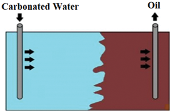
Figure 1: Water injection arrangement
A brief explanation of the gathering and arrangement of good information and production data is also included in this section. This focuses on helpful plots for assessing water production as well as techniques for tracking various costs associated with water handling and injection [16]. Wang et al. study the Inflow Performance Analysis of a Horizontal Well Coupling Stress Sensitivity and Reservoir Pressure Change particularly in a Fractured-Porous Reservoir [17].
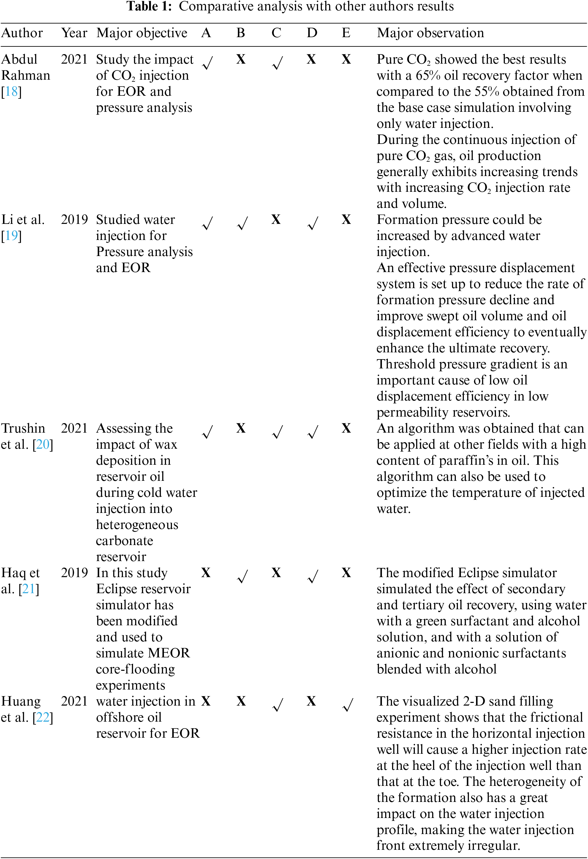
The comparative analysis of recent research works is defined in Tab. 1. Other simulation parameters are, A-Water injection, B-Pressure Analysis, C- Field Oil Production Total (FOPT) vs. Time analysis, D-Field Water Production Total (FWPT), and E-Formation Water Saturation (FWSAT).
The ratio of space in a rock to its bulk volume, multiplied by 100 to represent percent, is known as porosity. It is often referred to as the storage capacity of subsurface formations. Porosity is defined as 1) primary (formed during sediment deposition) or 2) secondary (produced after deposition of the rock) based on the method of genesis. Intergranular porosity in sandstones and carbonates, as well as inter particle and oolitic porosity in certain limestones, are examples of original porosity.
Fracture development in certain shales and limestones, as well as vugs or solution cavities in limestone and feldspar dissolving in sandstone, are all instances of induced porosity. Total or effective porosity are two different types of porosity. The characteristics of rocks with original porosity are more homogenous than those with porosity that have been produced in large amounts. Total porosity is defined as the proportion of space in a rock to its bulk volume (∅ as shown in Eq. (1).
where,
Vt = Total (or apparent) volume of the sample,
Vp = Volume of hollow spaces (or pore volume) between the solid grains,
Vs = Real volume of grains.
The ratio of the interconnected space in the rock to the bulk volume of the rock, both stated in percent, is known as effective porosity.
The ability of a rock medium to transfer or conduct fluids is measured by its permeability. Darcy or milli darcys are the units used to measure it. Flow pathways are randomly linked and come in a variety of forms and sizes. Horizontal and vertical fluid flow are both presents. The permeability of most porous rocks will vary over time. Matrix permeability is the flow in a rock’s major pore spaces, as opposed to fracture permeability, which is the flow in cracks or fractures. Solution channels and natural or manufactured cracks are common features in several grains of sand and carbonate reservoirs. The permeability of the matrix is not affected by these channels and fractures, but by the flow network’s effective permeability.
Prior to the invasion and entrapment of petroleum, the majority of oil-producing formations are thought to have been fully saturated with water. Less dense hydrocarbons push water out of the structurally high part of the rock’s interstices, causing it to shift to hydrostatic and dynamic equilibrium. The oil won’t be able to get rid of all of the water fully. As a result, petroleum hydrocarbons and water (also known as connate water) are commonly found in the same or neighboring pores in reservoir rocks. Before determining the number of hydrocarbons gathered in a porous rock formation, the fluid saturation of the rock material (oil, water, and gas) must be calculated. Displacement efficiency (Ed), invasion or vertical sweep efficiency (Ev), and pattern or areal sweep efficiency (Ep) all contribute to total recovery (Er), as shown in Eq. (2).
The residual oil saturation (Sor) of the swept zone determines displacement efficiency (Ed). So, Ed as a function of Sor and the interstitial (irreducible) water saturation (Swi) may be calculated using the following Eq. (3):
The ratio of viscous to capillary forces, called the capillary number, determines the displacement efficiency. The interfacial tension between the oil and the water is decreased in improved recovery procedures to increase the capillary number. Capillary pressure, relative permeability, and wettability must all be explained since two or more fluids might exist in porous rock at the same time.
The power required to push fluid down a pore throat and displace pore-wetting fluid is known as capillary pressure. To displace pore-wetting fluid, greater capillary pressures are necessary as pore mouths narrow. Capillary pressure curves can show pore throat sorting, relative permeability, and reservoir quality. Residual water saturation influences the size of the pore throat. Capillarity and distance above the oil-water contact determine the amount of water cut. Water injection methods such as waterflood operations rely heavily on capillarity.
The ratio of a fluid’s effective permeability to the rock’s base permeability is referred to as relative permeability. Relative permeability is a tough topic to grasp since it is both a rock characteristic and a fluid attribute. The kind of fluid moving, rock surface features, and pore structure geometry all influence a rock’s permeability. Permeability is also affected by the presence of several fluids in the pore space of rock. The fluid saturation determines the relative permeability, which ranges from zero to one. Relative permeability affects both oil and gas recovery as well as reservoir pressure.
Oil, water, and gas are the three most common phases found in reservoirs, and their effective Permeabilities are denoted by the letters ko, kw, and kg, respectively. Divide the effective permeability (k) to flow by the absolute permeability to get the relative permeability for each phase as shown in the set of Eq. (4).
Wettability is a measurement of which fluid clings to a rock surface preferentially when two immiscible fluids, such as oil and water, come into contact. The majority of producing reservoirs are water wet, which implies that connate water preferentially clings to the rock surfaces. The rock surface is considered to be water wet when the contact angle () between the rock surface and the water is less than 90 degrees, i.e., 90°. If the contact angle is more than 90 degrees, the rock is considered oil-soaked. Interstitial water saturation, residual oil saturation, and wettability are all influenced by wettability and other variables.
Wellbore diagrams are a wonderful way to record and display well data in an easy-to-understand format. Correctly analyzing relevant well and reservoir data can aid in the explanation of both production and reservoir performance. The importance of comprehensive individual well records of all production, injection, and workover data cannot be overstated. Knowing the overall output rate for the lease or field isn’t enough. Individual good rates are typically determined by testing each production well once or twice a month.
Data graph are visual displays that allow the operator to specify certain events that occur throughout a well’s life. Plots show the performance of individual wells as well as the entire project. There has also been evidence of interaction between the wells. Graphs can be created using hand-drawn plots, spreadsheet software, and oil and gas-specific software. The speed with which data may be updated and visually shown is a key benefit of having a computer to store it. The operator may produce charts for the entire project, individual wells, groups of wells, trends, and other study subjects fast and efficiently using the same data.
The operator will be able to observe and understand events that occur during the life of a well with the help of oil production plots. A semi-log representation of oil output vs. time is referred to as a “decline curve.” On a linear scale, the ordinate (or y-axis) reflects the logarithm of oil production rate, while the abscissa represents time (or x-axis). Extrapolating production decline patterns, calculating when the production rate will reach its economic limit, determining when the oil rate will peak, and determining when the initial production reaction from water injection will occur may all be done using this sort of graphic.
Plotting different rates against time can help identify key events connected to producing effectively. Water production, water-to-oil ratios (water cut), gas-to-oil ratios, water injection rates, and cumulative water injection are depicted in these graphs. Various rates vs. time are commonly displayed on the same graph. Different factors in a water injection process, such as injection and production rates, can be compared to see if they have a relationship. Changes in one rate might have an impact on another.
2.8.3 Water-Oil Ratio (WOR) vs. Cumulative Oil Production
To discover trends across a well’s lifespan, a semi-log plot of WOR versus cumulative oil output can be used. The ordinate shows WOR as a logarithm, whereas the abscissa indicates linear cumulative oil production. This graph shows the variations in water production as a function of oil output. Everything needed to follow a well is readily evident because the region under the curve represents complete water flow. A casing leak, a water break in a water drive reservoir, or a flood might all cause an increase in WOR.
A high WOR coupled with a low cumulative oil production might indicate a channeling problem. This plot should be created for both the whole project and each individual. If appropriately constructed, these graphs can also be used to forecast eventual recovery at a certain WOR. If a well’s WOR rises early in its life or is connected to low cumulative oil production, a thorough examination of individual excellent data, geological descriptions, and engineering data is necessary to identify the best course of action, which may include gelled polymer permeability adjustment. The WOR curve may reverse after good cleanup, followed by a flattening.
The type of process to be represented, as well as the process’s level of complexity, will impact the simulation model’s architecture. A 2-D aerial model may be used to depict the oil sweeping process in the drive as it occurs in the reservoir. The reservoir is separated into three sections: the oil zone, the aquifer, and the reservoir itself. The water volume change in the regional aquifer is calculated with the production of oil. With no real data provided for this simulation study, a 2000 ft. × 2000 ft. reservoir model with single layer is created with Eclipse 100 simulator. For case 1 and 2 models, the grid consisted of 40 blocks. The length and width of the model is 2000 ft. divided by 20 grid blocks which make the length and width of each grid block 1000 ft. and the height of the model is taken to be variable.
3.2 Reservoir Geometry and Properties
The reservoir model utilized in this study is basic. For simulation designs, the reservoir length, breadth, and thickness may be adjusted to various levels. The reservoir thickness is varied because the reservoir depth ranges from 7500 to 6880 feet. At 7000 feet, the water-oil contact was discovered, with reservoir thickness varying. At a reference depth of 6900 feet, the water-oil contact was discovered at 7000 feet, and reservoir pressure was recorded at 3000 psi. The aquifer chosen was of the Fetkovich type, and it was linked to the reservoir in the j+ direction.
The temperature gradient was set to 12° F every 100 feet, with the ground surface temperature fixed at 60° F. Although this number was not necessary for the simulation, the reservoir temperature is 120° F. Porosity was considered to be varied, ranging from 9% to 16%. The residual oil saturation was set to 25% and the irreducible water saturation to 20%. The horizontal permeability’s Kx and Ky are changeable with grid blocks and values as shown in the input data file, while the vertical permeability was set to a fixed value of 50 md.
PVT data was used to estimate the gas and water characteristics. Oil, water, and gas had specific gravities of 34.2, 1.07, and 0.7, respectively. The oil was thought to be dead, with very little dissolved gas. Capillary pressure was not taken into account in this investigation. In the first example, four producing wells were evaluated, whereas, in the second situation, four producing wells plus two injection wells were considered.
Although comer point geometry has excellence in simulation as this is a preliminary exercise block centered geometry is good enough. This approach will have a very less level of complexity, less data requirement, and a fair amount of reliability of results. The thickness of the grid blocks was taken variable varying in the range of 35–45 ft. approximately and Net-to-gross (NTG) ratio was taken as default. The period of the simulation was taken for five years. The period was chosen arbitrarily as it does not have any impact on the output produced. The reservoir was expected to be in the initial phase having no development done.
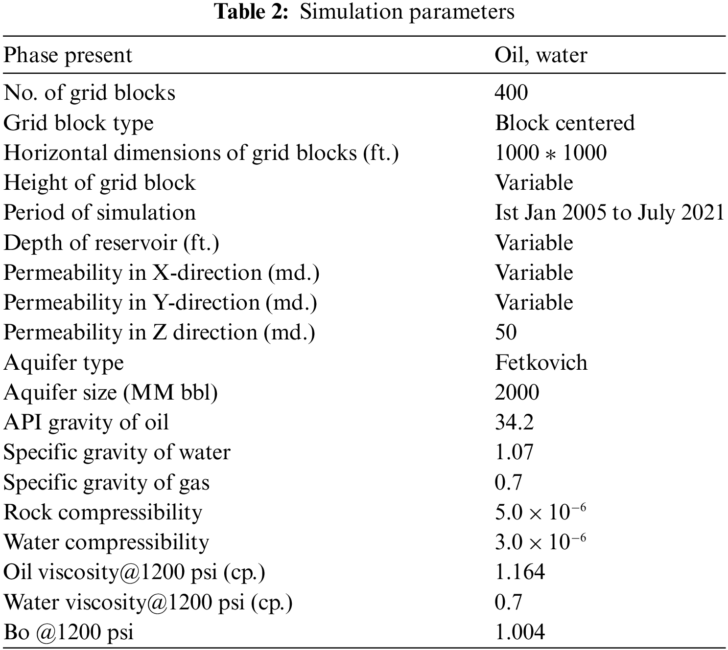
This section explains the simulation-based analysis using Eclipse software. Other simulation parameters are shown in Tab. 2.
4.1 Introduction of ECLIPSE 100 (Reservoir Simulation)
ECLIPSE 100 is a general-purpose black oil simulator with a gas condensate option that is entirely implicit, three-phased, and three-dimensional. The software is written in FORTRAN 77 and may be run on any computer that has an ANSI-compliant FORTRAN 77 compiler and enough RAM to run it. It might imitate one, two, or three system phases. Two-component systems are used to solve choices in two phases (oil/water, oil/gas, and gas/water), saving both computer storage and time. In addition to gas dissolving in oil (changing bubble point pressure or oil/gas ratio), ECLIPSE 100 may be used to mimic oil vaporizing in gas (shifting dew point pressure or oil/gas ratio or gas/oil ratio). Geometry choices include both corner-point and traditional block-center.
In one, two, or three dimensions, radial and Cartesian block-center choices are provided. The circle is completed with a 3D radial option that allows flow over the 0/360 degree interface. To start the simulation, we’ll need an input file with all of the reservoir’s data and the extraction technique. ECLIPSE’s input data is generated utilizing a free-format keyword system. The input file may be created using any standard editor. ECLIPSE Office may be used to interactively prepare data and submit runs.
The name of the input file must be formatted as follows: FILENAME.DATA. The section-header keyword is used to split parts in an ECLIPSE data input file. A list of all section-header keywords, as well as a description of each section’s contents and keyword occurrences in tile code, is provided below. It’s crucial to note that the input file’s keywords must be in the correct sequence. The input data file’s keywords (including section-header keywords) must all begin in column 1 and be no more than eight characters long. In the first eight columns, all of the characters have meaning. From column 9 onwards, any characters that appear on the same line as a keyword will be treated as comments.
A comprehensive study may take a year or more to complete and for a time may place intense demands on computer hardware and skilled personnel depending on the intensity of work required to achieve the desired result. Less comprehensive studies require fewer resources but usually must be conducted under severe time constraints.
Both types of studies should follow clear, practical plans to ensure that they supply the correct information to the reservoir management team in appropriate detail and above all, in time to be used effectively. Most studies involve essentially the same kinds of activities although the distribution of effort among the activities will vary from project to project depending on the objectives.
This study is to define the performance of the water drive reservoir and the associated operating parameters with and without water injection for reservoir pressure maintenance. The performance prediction will be based upon the reservoir parameters such as aquifer water influx, recovery, FOIP, formation pressure, water cut and formation water saturation. Tab. 2 defines the input data for simulation.
5.1 Simulated Results and Predictions
The results were obtained from Eclipse 100 software for two different cases:
CASE 1:4 wells producing at constant oil production rate.
CASE 2:4 wells producing at constant oil production rate with 2 injection wells with constant water injection rate.
The parameters selected for representing the performance of a reservoir are chosen as:
⮚ Total Oil Production (FOPT)
⮚ Total Water Injection (FWIT)
⮚ Field Water Cut (FWCT)
⮚ Avg. Reservoir Pressure (FPR)
⮚ Formation Oil in Place (FOIP)
⮚ Formation Water Saturation (FWSAT)
⮚ Oil Recovery (FOE)
⮚ Total Water Production (FWPT)
Also, individual good parameters such as well Bottom Hole Pressure (BHP), water cut, oil Productivity index (PI) are obtained for the simulation runs for both cases.
5.2 Total Oil Production (FOPT)
At the end of the last year total oil production of 24 MM STB (Million Stock Tank Barrels) was obtained and it increases linearly as the oil production rate was kept constant due to supply constraints as shown in Fig. 2. Such cases show similar results, as production constraints were the same as in case 1 and case 2.
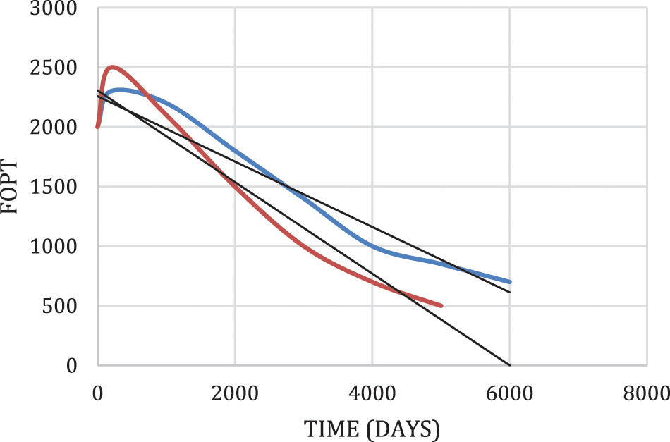
Figure 2: Average FOPT vs. Time (days) graph case I & case II
In case I, the water cut starts early around 3000 days, and increases very rapidly to attain a Value just above 0.38 in the next 3200 days. Such behavior of water cut may be resulting due to water coning as the good production rate is kept quite high. While in case 2, the water cut starts a little late at around 3500 days and increases rapidly to a value of 0.34 at the end of 6000 days as shown in Fig. 3. The reason behind late water coning may be a result of maintained pressure in the reservoir which is a more favorable case than case l.
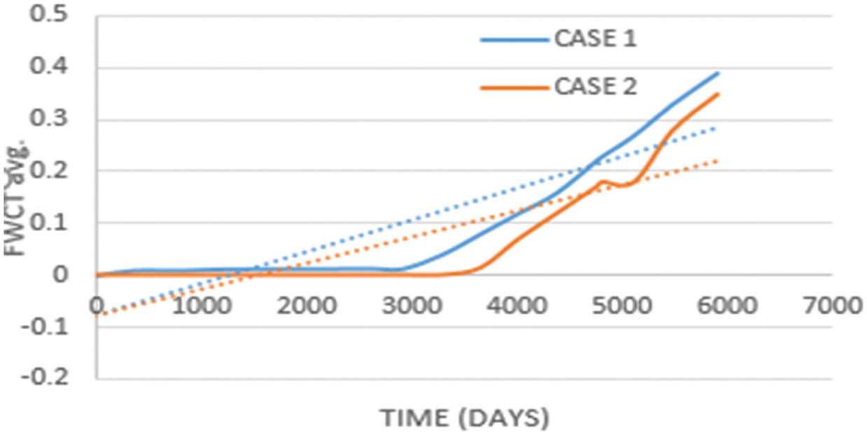
Figure 3: Average FWCT vs. Time (days)
5.4 Average Reservoir Pressure (FPR)
In this section average reservoir pressure decreases with the production life of the reservoir and attains a value of 1792 psi at the end 10th year (Case1). In case 2 due to water injection the depletion of pressure reduced from 1792 to 2136 psi as shown in Fig. 4. This will result in longer production life and ultimately increased overall recovery from the field.
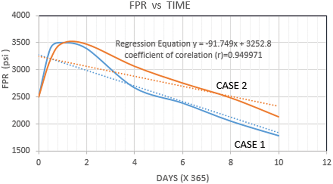
Figure 4: FPR vs. Time curve
5.5 Formation Oil in Place (FOIP)
The formation oil in place does not change as initial FOIP and total production from the reservoir are the same in both cases as shown in Fig. 5. Case 2 may result in less FOIP if production constraints for wells are changed from ORAT (Operational Readiness and Airport Transition) to BHP or liquid production rate. The remaining FOIP at the end of the 10th year was found to be 133 MM STB.
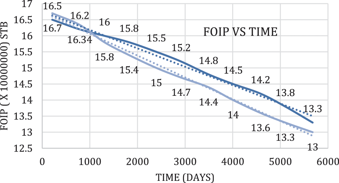
Figure 5: FOIP vs. Time curve
5.6 Formation Water Saturation (FWSAT)
The nature of formation water saturation remains the same for both cases as the exploitation scheme is the same excluding the injection wells. Case 1 results in an FWSAT value of 0.579 while case 2 results in 0.583 for ten years as shown in Fig. 6.
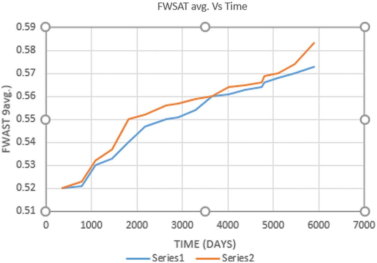
Figure 6: FWSAT vs. Time curve
The total oil recovery remains the same for both cases as the initial oil saturation and total oil production from the reservoir remain the same. The overall oil recovery at the end of July 2021 was to be just above 15% and change was found to be linear as the exploitation scheme was kept the same throughout the production life as shown in Fig. 7.
Now similar recovery does not suggest that both cases are the same in terms of ultimate recovery as case 2 definitely has larger production life and less residual oil in place and thus more ultimate recovery can be obtained.
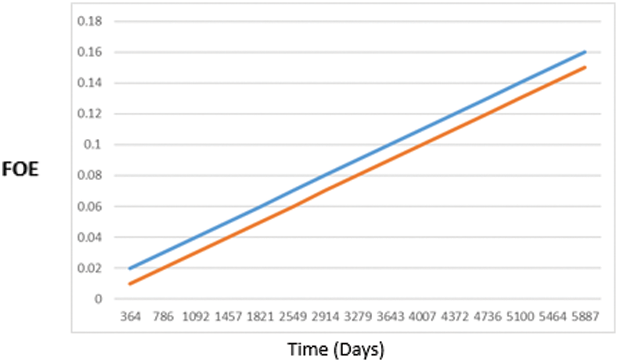
Figure 7: FOE vs. Time curve
5.8 Total Water Production (FWPT)
The water production in case 2 started a little early around 3500 days in comparison to case 1 where water production started around 4000 days. Case 2 shows premature and high water production due to the presence of water injection wells. At the end of the simulation study case, 1 result in a total water production of 2.3 MM STB, and case 2 result was the same 3.4 MM STB approx. as shown in Fig. 8. Even though the total water production in case 2 is higher but it shows much stable reservoir pressure and if this excess amount of produced water can be handled case 2 comes as a better exploitation scheme.
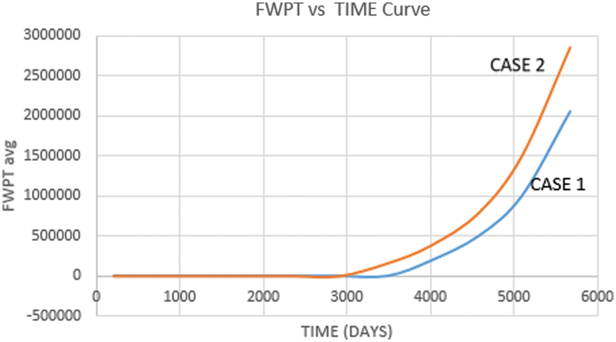
Figure 8: FWPT vs. Time curve
The objective of the study was to predict the performance of a model water drive reservoir based on the simulated results of Eclipse 100 simulators. The prediction was given based on two different cases representing two different exploitation schemes for the same reservoir under similar production constraints. The effort was to generate the simulated data for both cases to predict the favorable case in terms of different performance parameters. Based on the simulated results the case 2 was found out to be more favorable as it increases the production life of the reservoir and thus a higher total recovery can be expected before the abandonment of the reservoir is done. Also, if the production rate from the field is to be increased it is obvious that it will be easier and economically profitable in case 2 as it runs on a higher average reservoir pressure.
Being a preliminary exercise and due to limitations in the availability of data, it was not possible to simulate a more practical case in which the production figures will be more realistic. Also, if an actual set of reservoir data including production data is available and operating license permits history match should be practiced for validating the simulated results. Eclipse simulator provides more in-depth reach to the reservoir through dynamic modeling, front tracking, flow grid, well test data handling, etc. which can be used only after achieving proper license. The same reservoir model can be used to study the water flooding performance only by properly aligning the wells. Reservoir simulation models would also be used in the development of new fields. These models are also used in developed fields where production forecasts are needed to help make investment decisions.
Funding Statement: The author received no specific funding for this study.
Conflicts of Interest: Authors declare that they have no conflicts of interest regarding the present study.
Reference
1. K. A. Alwan, H. A. Baker and S. F. Fadhil, “Enhanced oil recovery using smart water injection,” Journal of Engineering, vol. 24, no. 8, pp. 40–54, 2018. [Google Scholar]
2. Y. Liu, L. Liu, J. Y. Leung, K. Wu and G. Moridis, “Coupled flow/geo-mechanics modeling of inter-fracture water injection to enhance oil recovery in tight reservoirs,” SPE Journal, vol. 26, no. 01, pp. 1–21, 2021. [Google Scholar]
3. Y. He, Y. Qiao, J. Qin and Y. Tang, “A novel method to enhance oil recovery by inter-fracture injection and production through the same multi-fractured horizontal well,” Journal of Energy Resources Technology, vol. 144, no. 04, pp. 043005, 2021. [Google Scholar]
4. H. Liu, X. Baocai and R. Chen, “Study on air foam flooding technology to enhance oil recovery of complex fault block reservoir by water injection,” IOP Conference Series: Earth and Environmental Science, vol. 781, no. 2, pp. 022032, 2021. [Google Scholar]
5. G. Dordzie and D. Morteza, “Enhanced oil recovery from fractured carbonate reservoirs using nanoparticles with low salinity water and surfactant: A review on experimental and simulation studies,” Advances in Colloid and Interface Science, vol. 293, pp. 102449, 2021. [Google Scholar]
6. R. Farajzadeh, S. Kahrobaei, A. A. Eftekhari and R. A. Mjeni, “Chemical enhanced oil recovery and the dilemma of more and cleaner energy,” Scientific Reports, vol. 11, no. 1, pp. 1–14, 2021. [Google Scholar]
7. M. Mahmoudpour and P. Pourafshary, “Investigation of the effect of engineered water/nanofluid hybrid injection on enhanced oil recovery mechanisms in carbonate reservoirs,” Journal of Petroleum Science and Engineering, vol. 196, no. 00, pp. 10766, 2021. [Google Scholar]
8. C. Esene, N. Rezaei, A. Aborig, and S. Zendehboudi, “Comprehensive review of carbonated water injection for enhanced oil recovery,” Fuel, vol. 237, pp. 1086–1107, 2019. [Google Scholar]
9. M. S. Sohrabi, A. Emadi and S. A. Farzaneh, “A thorough investigation of mechanisms of enhanced oil recovery by carbonated water injection,” in SPE Annual Technical Conf. and Exhibition, One Petro, 2015. [Google Scholar]
10. S. N. Hosseini, M. T. Shuker and M. Sabet, “Brine ions and mechanism of low salinity water injection in enhanced oil recovery: A review,” Research Journal of Applied Sciences, Engineering and Technology, vol. 11, no. 11, pp. 1257–1264, 2015. [Google Scholar]
11. E. C. Donaldson, G. V. Chilingarian and T. F. Yen, “Enhanced oil recovery, II: Processes and operations,” in Developments in Petroleum Science, LA, USA: Elsevier Science & Technology, vol. 17b, 1989. [Google Scholar]
12. P. Rostami, M. Sharifi, B. Aminshahidy and J. Fahimpour, “The effect of nanoparticles on wettability alteration for enhanced oil recovery: Micromodel experimental studies and CFD simulation,” Petroleum Science, vol. 16, no. 4, pp. 859–873, 2019. [Google Scholar]
13. J. O. Adegbite, E. W. Al-Shalabi and B. Ghosh, “Geochemical modeling of engineered water injection effect on oil recovery from carbonate cores,” Journal of Petroleum Science and Engineering, vol. 170, no. 00, pp. 696–711, 2018. [Google Scholar]
14. N. Morrow and J. Buckley, “Improved oil recovery by low-salinity waterflooding,” Journal of Petroleum Technology, vol. 63, no. 05, pp. 106–112, 2011. [Google Scholar]
15. G. van Essen, M. Zandvliet, P. Van den Hof and O. Bosgra, “Robust waterflooding optimization of multiple geological scenarios,” Spe Journal, vol. 14, no. 01, pp. 202–10, 2009. [Google Scholar]
16. W. Bangerth, H. Klie, M. F. Wheeler, P. L. Stoffa and M. K. Sen, “On optimization algorithms for the reservoir oil well placement problem,” Computational Geoscience, vol. 10, no. 3, pp. 303–19, 2006. [Google Scholar]
17. M. Wang, Z. Fan, W. Zhao, R. Ming and L. Zhao, “Inflow performance analysis of a horizontal well coupling stress sensitivity and reservoir pressure change in a fractured-porous reservoir,” Lithosphere, vol. Special, no. 1, pp. 7024023, 2021. [Google Scholar]
18. I. Abdulrahman, “An evaluation of the effects of carbon dioxide (CO2) injection on enhanced Oil recovery (EOR),” MS thesis. NTNU, 2021. [Google Scholar]
19. C. Li, J. Yang, J. Ye, J. Zhou, R. Zhang et al., “Semi-analytical modeling of advanced water injection in low permeability reservoirs under non-darcy-flow condition,” Advances in Mechanical Engineering, vol. 11, no. 5, pp. 1687814019846767, 2019. [Google Scholar]
20. Y. M. Trushin, A. S. Aleshchenko, O. N. Zoshchenko and M. S. Arsamakov, “A new approach to simulation of Wax precipitation during cold water injection in carbonate reservoir of kharyaga oilfield,” in SPE Russian Petroleum Technology Conf., OnePetro, 2021. [Google Scholar]
21. B. Haq, J. Liua and K. Liu, “Modification of eclipse simulator for microbial enhanced oil recovery,” J. Petrol Explor. Prod. Technol., vol. 9, pp. 2247–2261, 2019. [Google Scholar]
22. S. Huang, Y. Zhu, S. Chai, G. Ding, Y. Xin et al., “A practical model for water injection evaluation and optimization in typical offshore reservoirs considering formation heterogeneity based on experimental study,” in SPE Middle East Oil & Gas Show and Conf., OnePetro, 2021. [Google Scholar]
 | This work is licensed under a Creative Commons Attribution 4.0 International License, which permits unrestricted use, distribution, and reproduction in any medium, provided the original work is properly cited. |