DOI:10.32604/cmc.2022.025442
| Computers, Materials & Continua DOI:10.32604/cmc.2022.025442 | |
| Article |
A Hybrid System for Customer Churn Prediction and Retention Analysis via Supervised Learning
1Department of Computer Science, COMSATS University, Islamabad, Attock Campus, Pakistan
2Department of Computer Science, COMSATS University, Islamabad, Islamabad Campus, Pakistan
*Corresponding Author: Khalid Iqbal. Email: khalidiqbal@cuiatk.edu.pk
Received: 24 November 2021; Accepted: 11 February 2022
Abstract: Telecom industry relies on churn prediction models to retain their customers. These prediction models help in precise and right time recognition of future switching by a group of customers to other service providers. Retention not only contributes to the profit of an organization, but it is also important for upholding a position in the competitive market. In the past, numerous churn prediction models have been proposed, but the current models have a number of flaws that prevent them from being used in real-world large-scale telecom datasets. These schemes, fail to incorporate frequently changing requirements. Data sparsity, noisy data, and the imbalanced nature of the dataset are the other main challenges for an accurate prediction. In this paper, we propose a hybrid model, name as “A Hybrid System for Customer Churn Prediction and Retention Analysis via Supervised Learning (HCPRs)” that used Synthetic Minority Over-Sampling Technique (SMOTE) and Particle Swarm Optimization (PSO) to address the issue of imbalance class data and feature selection. Data cleaning and normalization has been done on big Orange dataset contains 15000 features along with 50000 entities. Substantial experiments are performed to test and validate the model on Random Forest (RF), Linear Regression (LR), Naïve Bayes (NB) and XG-Boost. Results show that the proposed model when used with XGBoost classifier, has greater Accuracy Under Curve (AUC) of 98% as compared with other methods.
Keywords: Telecom churn prediction; data sparsity; class imbalance; big data; particle swarm optimization
DATA volume is significantly growing in recent decade due to advancements in information technology. Concurrently, an enormous development is being made in machine learning algorithms to process this data and discover hidden patterns independently. Machine learning techniques learn through data and also have the potential to automate the analytical model building. Machine learning is divided into three categories such as: 1) supervised, 2) semi-supervised, and 3) unsupervised learning. Supervised learning is used to discover hidden patterns from labeled datasets. Whereas unsupervised learning is used to discover hidden patterns from unlabeled data. Therefore, unsupervised learning is beneficial in finding the structure and useful insights from an unknown dataset. However, semi-supervised learning falls in between unsupervised and supervised learning [1].
Customers are the most important profit resource in any industry. Therefore, telecom industry fear customer churn due to changing interests, and demand for new applications and services. Customer churn is defined as the movement of people from one company to another company for several reasons. The organization’s major concern is to retain their unsatisfied customers to survive in a highly competitive environment. To reduce customer churn, the company should be able to predict the behavior of customers correctly. For this, a churn prediction model is used to get an estimate of customers, who may switch a given service provider in the near future [2]. Along with the telecom industry, churn prediction has also been used in subscription-based services, e-commerce, and industrial area [3,4]. Nowadays, the use of the mobile phone is integral to our everyday life. This increases competition in the telecom sector, as it is less costly for a customer to switch services. The behavior of a churner typically relies on multiple attributes. From a company perspective, the expense of attracting new customers is 6 to 7 times higher than retaining the unsatisfied ones [5]. On the contrary, companies are aware of the fact of losing customers, resulting in decrease profits. Therefore, Customer Relationship Management (CRM) needs an effective model to predict future churners for automating the retention mechanism. Many operators also use simple pattern matching programs to identify potential churners. However, these programs require regular maintenance, and fail to incorporate the changing requirements. Therefore, machine learning algorithms have the potential to continually learn from new data and adapt as new patterns emerge.
In the past decade, significant research was performed to predict customer churn in telecom companies. Most approaches used machine learning for churn prediction [6]. One study combined two different ML models for customer churn prediction. The ML models are Back Propagation Artificial Neural Networks and Self Organizing Maps [7]. Various classification algorithms are used in this research [8] and compared their result to discover the most accurate algorithm for prediction of customer churn in businesses. In other research, the author creates a custom classification model using a combination of Artificial Neural Networks, Fuzzy modeling, and Tree-based models [9]. The proposed research is called the locally linear model tree (LOLIMOT). The results show that the LOLIMOT model achieved accurate classification as compared to other classification algorithms even in extremely unbalanced datasets. Similarly, researchers have suggested a large number of classifier-based techniques like Enhanced Minority Oversampling Technique (EMOTE), Support Vector Nachine (SVM), Support Vector Data Description (SVDD), Netlogo (agent-based model), Fuzzy Classifier, Random Forest (RF) (e.g., [10–18]). Also, there are hybrid techniques for churn prediction that merge two classifiers like K-Means with Decision Tree (DT), DT along with Logistic Regression (LR) and K-Means and classic rule inductive technique (FOIL) [19–21]. Also, Particle Swarm Optimization (PSO) based technique was proposed for feature selection in [22–25]. Nowadays, customer churn is a major issue for every organization. The operation of customer churn prediction has become more complicated. Therefore, there is a need to develop some new and effective that accurately predict customer churn that help the company in more effective allocation of its resources.
In this paper, our main concern is churn prediction for large datasets. We collected data from the international competition KDD Cup, 2009 (provided by Orange, Inc) [26]. We proposed a hybrid system, name as HCPRs, based on PSO feature selection and classification via different classifiers with the aim to generate better performance, and we addressed the class imbalance problem by using SMOTE. Furthermore, we reduce the overall computational cost through features selection. This method targets the issue of predicting customer churn, and retention analysis in telecom industry. The proposed system may help telecom companies to retain existing customers along with attracting new ones.
The following are our main contribution of this paper:
• We propose a hybrid model, named as A Hybrid System for Customer Churn Prediction and Retention Analysis via Supervised Learning (HCPRs) to address the issue of imbalance class data and feature selection. It uses a PSO based feature selection model which makes churn identification more quickly.
• We perform stratified five-fold cross validation for better testing of data, and performance evaluation.
• To demonstrate the effectiveness of HCPRs, we evaluate the proposed model against prominent techniques. Experimental results show an improved performance on RF compared to other classifiers.
The rest of the paper is organized as follows. In Section 2, we present previous work along with the statistics related to past work. Motivation and research questions are presented in Section 3. In Section 4, we describe the widely known performance metrics used in the Churn prediction problem. In Section 5, we discuss our proposed work. In Section 6, the prediction and evaluation are presented for multiple machine learning classifiers. In Section 7, experiments and results have been discussed. Finally, Section 8 concludes the paper and future work.
Churn in the telecom industry has been a long-term challenge for telecom companies. Typically, experts would manually perform churn analysis and make predictions accordingly. However, with the ever-increasing number of mobile subscribers and cellular data, it is not possible to predict manually. Hence, the research community has been attracted to explore the use of classifiers-based and PSO-based models for churn prediction.
2.1 Classifier Based Churn Prediction
In some previous researches, supervised learning approaches were used to identify churn like Naive Bayes, Logistic Regression, Support Vector Machines, Decision Tree and Random Forest (e.g., [27–29]). Awang et al. [30] presented a regression-based churn prediction model. This model utilizes the customer’s feature data for analysis and churns identification. Vijaya et al. [31] proposed a predictive model for customer churn using machine learning techniques like KNN, Random Forest, and XG Boost. The author compared the accuracy of several machine learning algorithms to determine the better algorithm of higher accuracy. One more research [16] proposed a fuzzy based churn prediction model and compared the accuracy of several classifiers with the fuzzy model. The author proved in predicting customer churn that fuzzy classifiers are more accurate as compared to others. De Bock et al. [32] design the GAMensplus classification algorithm for interpretability and strong classification. Karanovic et al. [5] proposed a questionnaire-based data collection technique processed over Enhanced Minority Oversampling Technique (EMOTE) classifier. Maldonado et al. [33] proposed relational and the non-relational learner’s classifiers handling data sparsity by social network analytic method.
In earlier days, many researchers show that single model based churn prediction techniques do not produce satisfactory results. Therefore, researchers switched on to hybrid models [18–20]. The basic principle with the hybrid model is to combine the features of two or more techniques. One study combined two different ML models for customer churn prediction such as Back Propagation Artificial Neural Networks and self-organizing Maps [7]. A data filtration process was performed using a hybrid model combining two neural networks. After that, data classification was performed using Self-Organized Maps (SOM). The proposed hybrid model was evaluated through two fuzzy testing sets and one general testing set. The evaluation results show that the proposed hybrid model was outperforming in prediction and classification accuracy, using a single neural network baseline model. In one more research, the author creates a custom classification model using a combination of Artificial Neural Networks, Fuzzy modeling, and Tree based models [9].
2.3 PSO-Based Churn Prediction
PSO-based techniques were proposed to solve the problem of customer churn (e.g., [21,24,28,31]). Huang et al. [21] proposed a technique for churn prediction using particle swarm optimization (PSO). Furthermore, the author proposed three variants of PSO that are 1) PSO incorporated with feature selection, 2) PSO embedded with simulated annealing and 3) PSO with a combination of both feature selection and simulated annealing. It was observed that proposed PSO and its variants give better results in imbalanced scenarios. Guyon et al. [34] designed a model for efficient churn prediction by using data mining techniques. In preprocessing stage, the k-means algorithm is used. After preprocessing, attributes are selected by employing the minimum Redundancy and Maximum Relevance (mRMR) approach. This technique uses the Support Vector Machine with Particle Swarm Optimization (SVM with PSO) to examine the customer churn separation or prediction. The experiments show that the proposed model attain better performance as compared to the existing models in terms of accuracy, true-positive rate, false-positive rate, and processing time. Vijaya et al. [31] handled imbalanced data distribution by features selection using PSO. It used Principle Component Analysis (PCA), Fisher’s ratio, F-score, and Minimum Redundancy and Maximum Relevance (mRMR) techniques for feature selection. Moreover, Random Forest (RF) and K Nearest Neighbor (KNN) classifiers are utilized to evaluate the performance.
In this section, we present the overall architecture of the proposed model along with its major component descriptions.
The performance of the proposed model is evaluated in a telecom churn prediction model after knowing the problem statement in this era. Telecom providers T = {t1, t2, t3,…,tk} competing each other that may result in customers churn where C = {c1, c2, c3,…., cn}. Telecom providers (ti ⊆ T) require an identification system for churners (c ⊆ C) having a high possibility to churn. Considered multiple features F = {f1, f2, f3,….fj} of customers either to churn or non-churn along with a class label (L). The feature selection process is done to get the prediction result on considering valuable features (f ⊆ F).
The overall work flow diagram of the proposed system is illustrated in Fig. 1. We explain the components of the churn prediction proposed model in a step-by-step manner. In the first step, data pre-processing is performed that comprises the data cleaning process, removal of imbalanced data features, and normalized the data. The synthetic Minority Oversampling (SMOTE) technique is used to balance the imbalanced data in telecommunication industries to improve the performance of churn prediction. In the second step, important features are extracted from data using the particle swarm optimization (PSO) mechanism. In the third step, different classification algorithms are employed for categorizing the customers into the churn and non-churn customers. The classification algorithms consist of Logistic Regression (LR), Naïve Bayes (NB), Random Forest (RF), and XG-boost.

Figure 1: Precise churn prediction proposed model
A publicly available Orange Telecom Dataset (OTD) is provided by the French telecom company [35]. The orange dataset consists of churners and non-churners. The dataset contains a large amount of information related to the customers and mobile network services. This information is considered in the KDD cup held for customer relationship prediction [36]. The dataset consists of 15000 variables and 50000 instances; the dataset is further divided into five chunks (C1, C2, C3, C4, C5) that contain an equal number of samples (10,000 each). Furthermore, out of 50000 samples, 3672 and 46328 samples were churners and non-churners. The approximate percentage ratio between churner and non-churner in OTD is 7:93. Due to which class imbalance problem occurs in such data set, Fig. 2 shows a graphical representation between churner vs. non-churners. The names of the features are not defined to respect the customer’s privacy. OTD is a heterogeneous dataset that consists of noisy data with variations in the measurement scale, features with null values, features with missing values, and data sparsity. Hence, for which data pre-processing is a requirement on such kind of dataset.

Figure 2: Churner vs. non-churner in OTD
The dataset consists of noisy features, sparsity and missing values. In the dataset it was noticed that approximately 19:70% of the data have missing values. The main purpose of data pre-processing step is to consider data cleaning for missing values and noisy data and data transformation. For data normalization, there are several methods like Z-Score, Decimal Scaling and Min-Max. Resolving the data sparsity problem, we used Min-Max normalization method. Min-Max normalization method performs a linear transformation on the data. In this method, we normalize the data in a predefined interval that is valued 0 and 1.
Class Imbalance
Distribution of the dataset where one class has a very large number of instances compared to the other class. The class with few samples is the minority class, and the class with relatively additional instances is the majority class. The imbalance between two classes is represented by the use of the “Ratio Imbalance” which is defined as the ratio between a number of samples of the majority class and that of a minority class. In forecasting the customer churn rate, the number of nonsense are relatively high compared to the churn number. Several techniques have been proposed to solve the problems associated with an unbalanced dataset. These techniques can be classified into four categories such as [36]:
• Data level approaches,
• Algorithm level approaches,
• Cost-sensitive learning approaches, and
• Classifier Ensemble techniques
Data level oversampling technique reduces the imbalance ratio of the skewed dataset by duplicating minority instances. The most commonly used an oversampling technique is the Synthetic Minority Oversampling Technique (SMOTE) [37]. A SMOTE introduces additional synthetic samples into the minority class instead of directly duplicating instances.
Using synthetic samples helps create larger and less specific decision regions. The algorithm first finds k nearest neighbors from each minority class sample using Euclidean distance as a measure of distance. Synthetic examples are generated along the line segments connecting the original minority class sample to its nearest k neighbors. The value of k depends on the number of artificial instances that need to be added. Steps for generating synthetic samples [36]:
1. Generate a random number between 0 and 1
2. Compute the difference between the feature vector of the minority class sample and its nearest neighbor
3. Then Multiply this difference by a random number (as generated in step 1)
4. After multiplication, adds the result of multiplication of the feature vector of the minority class sample
5. The resulting feature vector determines the newly generated sample
In this paper, we considered the Orange dataset, the distribution of the number of churners and the number of non-churner had a large amount of difference in the dataset. Computed values between the churner against the nonchurner are 3672 (7:34%) and 46328 (92:65%), respectably. It shows the ratio of 1:13 between churners and non-churns. In customer churn prediction, the number of non-churners is relatively high with respect to the number of churners as shown in Fig. 3.

Figure 3: Chunk wise OTD churner vs. non-churner
For such an unbalanced distribution of the two classes, the few churners getting the same weight in a cost function as the non-churner will result in a high misclassification rate. As the classifier will be biased towards the majority class. To resolve this imbalance issue, we used an advanced oversampling technique SMOTE. The working of generic SMOTE is demonstrated in Fig. 4. A synthetic oversampling technique performed rather than simple Random Under Sampling (RUS) and Random Over Sampling (ROS) technique. We resolved the imbalance issue by making the minority class (churners) equal to the majority one (nonchurner) with a ratio of 1:1.

Figure 4: Generic SMOTE synthetic churner instance creation
3.4 PSO Based Feature Selection
Choosing subsets of features from an original dataset or eliminating unnecessary features are the fundamental principle underlying feature selection. Having irrelevant functionality in the dataset can reduce the accuracy of classification models and force the classification algorithm to process based on irrelevant functionality. A subset that must represent the original data necessarily and reasonably while still being useful for analytical activities. The feature selection activity focuses on finding an optimal solution in a generally large search space to mitigate classification activity. Therefore, it is recommended that performs a feature selection task before training a model. In this work, we use PSO-based feature selection mechanism of generating the best optimum subset for each of the chunks individually. It is a suitable algorithm for addressing feature selection problems for the following reasons: easy feature encoding, global search function, computationally reasonable, fewer parameters, and easy implementation [3]. The PSO is implemented for feature selection because of the above reasons.
The algorithm was introduced as an optimization technique for natural number spaces and solved complex mathematical problems. This algorithm work on the principle of interaction to share information between the members. This method performs the search of the optimal solution through particles. Each particle can be treated as the feasible solution to the optimization problem in the search space. The flight behavior of particles is considered as the search process by all members. PSO is initialized with a group of particles, and each particle moves randomly. A particle i is defined by its velocity vector, vi, and its position vector to xi. Each particle's velocity and position are dynamically updated in order to find the best set of features until the stopping criterion is met. The stopping criteria can be a maximum number of iterations or a good fitness value.
In PSO, each particle updates its velocity VE and positions PO with following equations:
where i denote the index of the swarm global best particle, VE is the velocity and
where Np is the total number of particles, f is the fitness function, p is the position and t is the current iteration number.
The first part of Eq. (1) (i.e.,
After the feature selection stage, we will obtain meaningful global best selected features X = [x1, x2, x3, …., xi] (i.e., (X(f)). Hence, after doing all the above process step by step we are in a position to have a purified Orange Telecom Dataset, visualized in Fig. 5. In purified dataset class, imbalance issue is removed, the dataset has no null or missing values, dataset values are normalized in-between [0, 1], and the most relevant features have been selected.

Figure 5: Purified OTD
It is necessary to evaluate the model in order to determine which one is more reliable. Cross-validation is one of the most used methods to assess the generalization of a predictive model and avoid overfitting. There are three categories of cross-validation: 1) Leave-one-out cross-validation (LOOCV), 2) k-Fold cross-validation, and 3) Stratified cross-validation. This study focuses primarily on the stratification k-fold cross-validation (SK).
The Stratification k-fold cross-validation (SK) works as the following steps:
1) SK splits the data into k folds, making particular, each fold is a proper representation of the original data
• The proportion of the feature of interest in the training and test sets is the same as in the original dataset.
2) SK selects the first fold as the test set.
• The test set selects one by one in order. For instance, in the second iteration, the second fold will be selected as the test
3) Repeat steps 1 and 2 for k times
In this paper, stratified k-fold forward cross-validation is used, which is an improved version over traditional k-fold cross-validation for evaluating explorative prediction power of models. Instead of randomly partitioning the dataset, the sampling is performed so that the class proportions in the individual subsets reflect the proportions in the learning set. Stratified k-fold cross-validation is an improved version of traditional k-fold cross-validation. SK can preserve the imbalanced class distribution for each fold. Instead of randomly partitioning the dataset, stratified sampling is performed in such a way that the samples are selected in the same proportion as they appear in the population as shown in Fig. 6. For example, if he learning set contains n = 100 cases of two classes, the positive and the negative class, with n+ = 80 and n− = 20. If random sampling is done without stratification, then some validation sets may contain only positive cases (or only negative cases). With stratification, however, each validation set of 5-fold cross-validation is guaranteed to contain about eight positive cases and two negative cases, thereby reflecting the class ratio in the learning set.

Figure 6: Visualization of a stratified k-fold validation when k = 5
In this section, we used multiple classifiers that are Naïve Bayes (NB), Logistic Regression (LR), Random Forest (RF), and XG-Boost to get accurate and efficient prediction results of customer’s churners.
Naive Bayes (NB) [38,39] is a type of classification algorithm based on the Bayesian theorem. It determines the probabilities of classes on every single instance and feature [x1, x2, x3, . . . , xi] to derive a conditional probability for the relationships between the feature values and the class. The model contains two types of probabilities that can be calculated directly from the training data: (i) the probability of each class and (ii) the conditional probability for each class given each x value. Here, the Eq. (4) used for Bayes Theorem is given as,
where
Hence, the equation of Bayes theorem can also be written
In this paper, Naïve Bayes algorithm was implemented to predict either the customer will churn or not.
Logistic regression (LR) is the machine learning technique that solved binary classification problems. LR takes the real valued inputs and estimates the probability of an object belonging to a class. In this paper, a regression algorithm is evaluated to classify the customer churn and non-churners.
where y is the dependent variable and x is the set of independent variables. The value of y is ‘1’ implies the churned customer or y is ‘0’ implies the non-churn customer.
LR is estimated through the following equation:
where β is the coefficients to be learned and Pr is the probability of churn or not churn. If the value of probability pr is >0.5 then it takes the output as class 0 (i.e., non-corners) otherwise it takes the output as class 1 (i.e., churners).
Random Forest (RF) [40,41] is a classification algorithm that builds up many decision trees. It adds a layer of randomness that aggregates the decision trees using the “bagging” method to get a more precise and stable prediction. Therefore, RF performs very well compared to many other classifiers. Both classification and regression tasks can be accomplished with RF. It is robust against overfitting and very user-friendly [41].
The random forest technique's main idea is as follows:
1. Feature selection is accomplished on the decision tree to purify the classified data set. GINI index is taken as the purity measurement standard:
where G represents the GINI function; q represents the number of categories in sample D; Pi represents the proportion of category i samples to the total number of samples and k represents that sample D is divided into k parts, that is, there are k Dj data sets.
When the value of the GINI index (Eq. (8)) reach the maximum, then the node splitting is accomplished.
2. The generated multiple decision trees establish the random forest, and a majority voting mechanism is adopted to complete the prediction. The final classification decision is shown in Eq. (9).
where L(X) represents the combined classification algorithm; li represents the classification algorithm of ith decision tree, and y is the target variable. I(•) is the indicative function. Fig. 7 presents the generic working of the RF ensemble model on a purified orange dataset with final predictions.

Figure 7: Generic overview of RF in churn prediction
In this work, we adopt the Extreme Gradient Boosting (XGBoost) an algorithm as a machine learning algorithm that is employed for classification and regression problems. XGBoost is also a decision-tree-based ensemble algorithm that uses a gradient boosting framework that boosts weak learners to become stronger. XGBoost experimented on the Orange Telecom Dataset. XGBoosting algorithm only takes numerical values that are a suitable technique to use the orange dataset. It is famous due to the speed and performance factors.
XGBoost used the primary three gradients boosting techniques such as 1) Regularized, 2) Gradient, and 3) Stochastic boosting to enhance and tune the model. Moreover, it can reduce and control overfitting and decrease time consumption. The advantage of XGboost is that it can use multiple core parallel and fasten the computation by combining the results. Accuracy gained with the XGBoost algorithm was better than all the previous methods.
3.6.5 Multiple Linear Regression
MLR determines the effect when a variety of parameters are involved. For example, while predicting the behavior of churn users, multiple factors could be considered such as: cost, services, customer dealing which a telecom company provides. The effect of these different variables is used to calculate y (dependent variable) is calculated by multiplying each term with assigned weight value and adding all the results.
In this study, Accuracy, Precision, Recall, F1-Measure, and Accuracy Under Curve (AUC) based evaluation measures are used to quantify the accuracy of the proposed HCPRs churn prediction model. These well-known performance metrics are employed due to their popularity considered in existing literature for evaluating the quality of the classifiers that are used for churn prediction [42–44]. The following evaluation measures are used:
Accuracy is defined as the ratio of the correct classifications of the number of samples to the total number of samples for a given test dataset. It is mainly used in classification problems for the correct prediction of all types of predictions. Mathematically, it is defined in Eq. (10).
where ‘TN’ is True Negative, ‘TP’ is True Positive, ‘FN’ is False Negative and ‘FP’ is False Positive.
Precision is defined as the ratio of the correct classifications of positive samples to all numbers of the classified positive samples. It describes that the part of the prediction data is positive. Mathematically, it is defined in Eq. (11).
Recall measures the ratio of correctly classified relevant instances to the total amount of relevant instances. It can be showed for the churn and non-churn classes by the following equations, respectively.
The F1 score is defined as a weighted average precision and recall. Where the F1 best score value is 1, and the worst score value is 0. The relative part of precision and recall to the F1 score are equal. Mathematically, it is defined in Eq. (13).
4.5 Accuracy Under Curve (AUC)
We also used the standard scientific accuracy indicator, AUC (Area under the Curve) ROC (Receiver Operating Characteristics) curve to evaluate the test data. An excellent model with the best performance has higher the area under the curve (AUC) in an ROC.
Mathematically, it is defined in Eq. (14).
where P represents the number true churners and N shows the number of true non-churners. Arranging the churners in descending order, rank n is assigned to the highest probability customer, the next with rank n-1 and so on.
The proposed HCPRs approach is validated with the comprehensive experimentation carried on respective combinations of sampling, feature selection, and classification methodologies. In this section, a comparative analysis of HCPRs with other existing approaches are also included. Orange Telecom Dataset (OTD) is used, as discussed in Section 3.4 performance evaluation of the proposed churn prediction model. In this study, 5-fold cross-validation testing is adopted for analyzing the performance of the proposed model. OTD dataset is further divided into five chunks (C1, C2, C3, C4, C5) that contains an equal number of samples.
5.1 Classifiers Performance Evaluation on Split OTD
We used multiple classifiers by not rely only on a single classifier as evaluation results vary from classifier to classifier. Classifiers considered in our study are Naïve Bayes (NB), Logistic Regression (LR), Random Forest (RF), and XG-Boost. Performance metrics used to predict the efficiency of the model chunk wise are Accuracy, Recall, Precision, F-Measure, whose results can be visualized in Fig. 8. It can be seen that chunk 3 shows a high accuracy rate of Random Forest, XGBoost, Logistic Regression 95%, 96%, 88%, respectively whereas Naïve Bayes has a low accuracy rate of 74%. From the experimental results, the XGBoost outperformed the other classification algorithms on accuracy evaluation measures. Random Forest, XGBoost, Logistic Regression performed very well at Precision 96%, 9%, and 90%, respectively. Although Naïve Bayes has a lower precision rate of 83%. Although XGBoost outperformed the other algorithms on precision. XGBoost and Random Forest classifier gives higher recall score, i.e., 96%, 95% compared to Naïve Bayes and Logistic Regression classifiers. As displayed in Fig. 8, we confirm that the XGBOOST algorithm and Random Forest outperformed the rest of the tested algorithms with an F1-measure value of 95%. Logistic Regression algorithm occupied second place with an F1-measure value of 88%, while Naïve Bayes came last in the F1-measure ranking with a value of 73%.
From the experimental results, XGBoost algorithm outperformed the other classification algorithms on most evaluation measures.

Figure 8: Classifier performance evaluation on split OTD
5.2 Split OTD Area under ROC Curve Visualization with Multiple Classifiers
This section presents the ROC curve of LR, Naive Byes, Random Forest and XGBOOST. ROC curve is widely used to measure the test’s ability as a criterion. In general, the ROC curve is used to predict the model accuracy. The area under the ROC curve (AUC) is a measure of how well parameters can distinguish between churned and not churned groups. The AUC value is between 0:5 and 1. AUC value is better if it is close to 1. Moreover, the mean value of folds is also computed on the classifiers. Fig. 9 shows an overall view of the ROC curve on multiple classifiers that visualized on a split orange dataset along with mean AUC values. Stratified 5-fold cross-validation is used on each of the chunks. After 5-fold cross-validation, the Naïve Bayes Classifier means the AUC value of each chunk is 0:75 as shown in Fig. 9.

Figure 9: Split OTD area under ROC curve visualization with multiple classifiers
After that, we implemented a Logistic Regression classifier to obtain more accurate results. Similarly, like the previous technique, the environment is the same, and the mean AUC value is predicted 0:93 of C1, C2, and C4, and the mean AUC obtained on C3 and C5 is 0:94. Moreover, to predict churner more accurately, we also used an ensemble technique, Random Forest. ROC curve showed much more required results of each chunk with a mean AUC value of 0:962. Furthermore, we also used a boosting technique (i.e., XGBoost) on the same split orange dataset to obtain more accurate results. ROC curve gave more accurate and efficient results than all the previous techniques. The mean AUC value of each chunk (i.e., C1, C2, C3, C4, C5) is 0:98. Results showed that the ensemble technique outperformed on the Orange dataset. Fig. 10 demonstrates the graphical representation of mean AUC results reported by the classifiers used in our research.

Figure 10: Multiple classifiers mean AUROC curve
5.3 Performance Comparison with other Existing Approaches
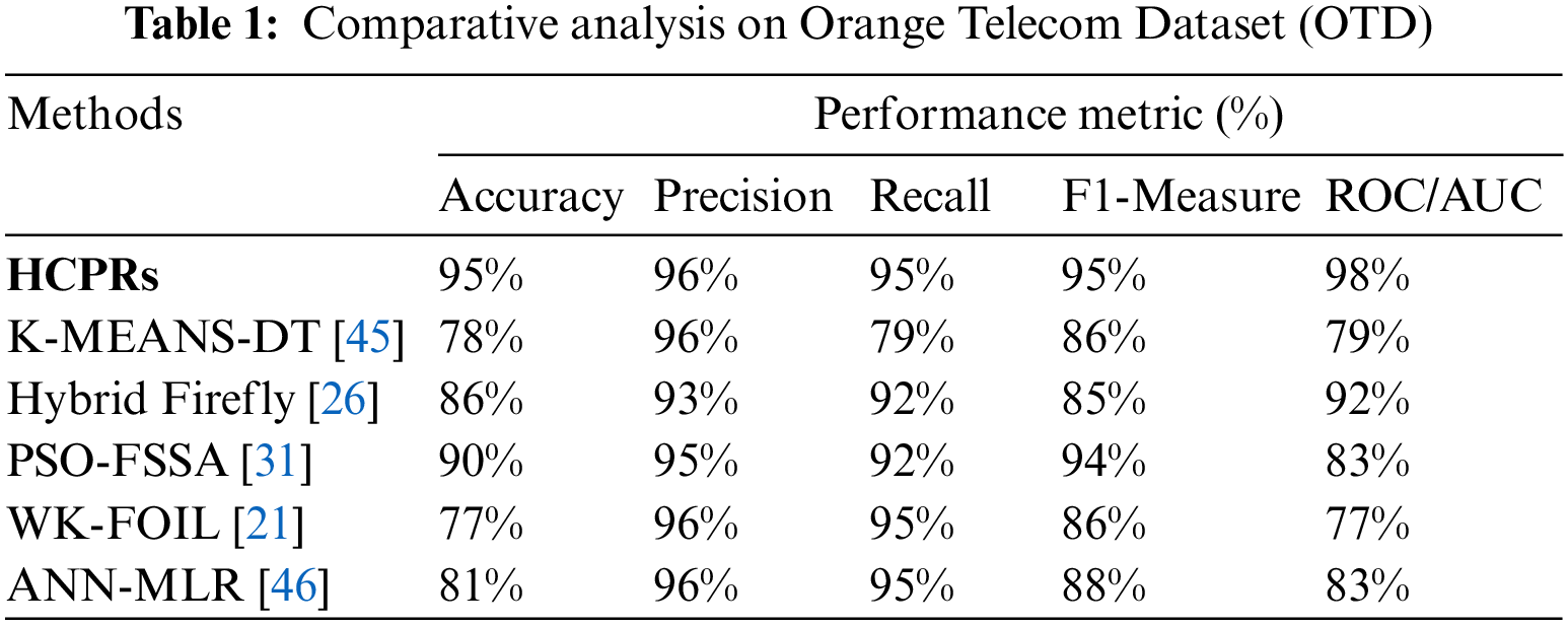
Numerous approaches applied with different classifiers in the domain of churn prediction. The comparison was taken based on performance evaluation metrics such as accuracy, precision, recall, F1-measure, and the ROC/AUC with the same dataset and different telecom datasets. These metrics were chosen to identify the performance of the HCPRs technique. Comparison of the HCPRs technique with K-MEANS-DT [45], Hybrid Firefly [26], PSO with a combination of both feature selection and simulated annealing (PSO-FSSA) [31], Weighted K-means and a classic rule inductive technique (FOIL) (WK-FOIL) [21] and Artificial Neural Networks and Multiple Linear Regression models (ANN-MLR) [46] were performed to measure the difference in performance levels Tab. 1 shows the comparison of the current technique with different approaches with the same dataset.
From the experimental results, the proposed HCPRs significantly perform better as compared to the other algorithms on most evaluation measures in predicting telecom churners when evaluated on an Orange Telecom Dataset (OTD). Although it performed not very well at Precision, it outperformed the other algorithms on Accuracy, Recall, F1-score, and ROC/AUC. In addition, the predictive performance of our proposed model of the ROC curve is most excellent.
A hybrid PSO based churn prediction model is presented in this paper. We tested our model on an orange telecom dataset. For preprocessing, SMOTE technique is used for data cleaning, and removal of imbalanced data features. After that important features are extracted from data with PSO. Furthermore, Logistic Regression (LR), Naive Bayes (NB) and Random Forest (RF) are used for categorizing customers into two categories i.e., churn, and non-churn customers. It is shown through results that using a stratified 5-fold cross validation procedure improves the performance of our prediction model. Naive Bayes is given 0:75 least accurate result on AUC in comparison with Logistic Regression and Random Forest giving 0:934 and 0:962 respectively.
For the future work, we plan to automate the retention mechanism based on these prediction methods, which is now a days a necessary requirement of a telecom company. Furthermore, we intend to perform experiments with increasing number of folds up to 10-folds for gaining accurate results.
Funding Statement: The authors received no specific funding for this study.
Conflicts of Interest: The authors declare that they have no conflicts of interest to report regarding the present study.
1. A. Saran Kumar and D. Chandrakala, “A survey on customer churn prediction using machine learning techniques,” International Journal of Computer Applications, vol. 154, no. 10, pp. 13–16, 2016. [Google Scholar]
2. L. Katelaris and M. Themistocleous, “Predicting customer churn: Customer behavior forecasting for subscription-based organizations,” in European, Mediterranean, and Middle Eastern Conf. on Information Systems, EMCIS 2017: Coimbra, Portugal, pp. 128–135, 2017. [Google Scholar]
3. N. Gordini and V. Veglio, “Customers churn prediction and marketing retention strategies. An application of support vector machines based on the AUC parameter-selection technique in B2B e-commerce industry,” Industrial Marketing Management, vol. 62, no. 3, pp. 100–107, 2017. [Google Scholar]
4. A. Bansal, “Churn prediction techniques in telecom industry for customer retention: A survey,” Journal of Engineering Science, vol. 11, no. 4, pp. 871–881, 2020. [Online]. Available: https://www.jespublication.com. [Google Scholar]
5. M. Karanovic, M. Popovac, S. Sladojevic, M. Arsenovic and D. Stefanovic, “Telecommunication services churn prediction-deep learning approach,” in 2018 26th Telecommunications Forum (TELFOR), Belgrade, Serbia, pp. 420–425, 2018. [Google Scholar]
6. P. Lalwani, M. K. Mishra, J. S. Chadha and P. Sethi, “Customer churn prediction system: A machine learning approach,” Computing, vol. 104, no. 8, pp. 1–24, 2021. [Google Scholar]
7. C. F. Tsai and Y. H. Lu, “Customer churn prediction by hybrid neural networks,” Expert Systems with Application, vol. 36, no. 10, pp. 12547–12553, 2009. [Google Scholar]
8. S. R. Labhsetwar, “Predictive analysis of customer churn in telecom industry using supervised learning,” ICTACT Journal of Soft Computing, vol. 10, no. 2, pp. 2054–2060, 2020. [Google Scholar]
9. A. Ghorbani, F. Taghiyareh and C. Lucas, “The application of the locally linear model tree on customer churn prediction,” in 2009 Int. Conf. of Soft Computing and Pattern Recognition, Las Vegas, pp. 472–477, 2009. [Google Scholar]
10. S. Babu and N. R. Ananthanarayanan, “Enhanced prediction model for customer churn in telecommunication using EMOTE,” in Int. Conf. on Intelligent Computing and Applications, Sydney, Australia, pp. 465–475, 2018. [Google Scholar]
11. R. Dong, F. Su, S. Yang, X. Cheng and W. Chen, “Customer churn analysis for telecom operators based on SVM,” in Int. Conf. on Signal and Information Processing, Networking and Computers, Chongqing, China, pp. 327–333, 2017. [Google Scholar]
12. S. Maldonado and C. Montecinos, “Robust classification of imbalanced data using one-class and two-class SVM-based multiclassifiers,” Intelligent Data Analysis, vol. 18, no. 1, pp. 95–112, 2014. [Google Scholar]
13. S. Maldonado, Á. Flores, T. Verbraken, B. Baesens and R. Weber, “Profit-based feature selection using support vector machines--General framework and an application for customer retention,” Applied Soft Computing, vol. 35, no. 3–4, pp. 740–748, 2015. [Google Scholar]
14. M. Óskarsdóttir, C. Bravo, W. Verbeke, C. Sarraute, B. Baesens et al., “Social network analytics for churn prediction in telco: Model building, evaluation and network architecture,” Expert Systems with Appications, vol. 85, no. 10, pp. 204–220, 2017. [Google Scholar]
15. S. D’Alessandro, L. Johnson, D. Gray and L. Carter, “Consumer satisfaction versus churn in the case of upgrades of 3G to 4G cell networks,” Marketing Letters, vol. 26, no. 4, pp. 489–500, 2015. [Google Scholar]
16. M. Azeem, M. Usman and A. C. M. Fong, “A churn prediction model for prepaid customers in telecom using fuzzy classifiers,” Telecommunication Systems, vol. 66, no. 4, pp. 603–614, 2017. [Google Scholar]
17. M. Azeem and M. Usman, “A fuzzy based churn prediction and retention model for prepaid customers in telecom industry,” International Journal of Computational Intelligence System, vol. 11, no. 1, pp. 66–78, 2018. [Google Scholar]
18. E. Shaaban, Y. Helmy, A. Khedr and M. Nasr, “A proposed churn prediction model,” International Journal of Engineering Research and Applications, vol. 2, no. 4, pp. 693–697, 2012. [Google Scholar]
19. Y. Huang, “Telco churn prediction with big data,” in Proc. of the 2015 ACM SIGMOD Int. Conf. on Management of Data, Australia, Melbourne, pp. 607–618, 2015. [Google Scholar]
20. A. De Caigny, K. Coussement and K. W. De Bock, “A new hybrid classification algorithm for customer churn prediction based on logistic regression and decision trees,” European Journal Operational Research, vol. 269, no. 2, pp. 760–772, 2018. [Google Scholar]
21. Y. Huang and T. Kechadi, “An effective hybrid learning system for telecommunication churn prediction,” Expert Systems with Applications, vol. 40, no. 14, pp. 5635–5647, 2013. [Google Scholar]
22. J. Pamina, J. B. Raja, S. S. Peter, S. Soundarya, S. S. Bama et al., “Inferring machine learning based parameter estimation for telecom churn prediction,” in Int. Conf. on Computational Vision and Bio Inspired Computing, Coimbatore, India, pp. 257–267, 2019. [Google Scholar]
23. A. Idris, M. Rizwan and A. Khan, “Churn prediction in telecom using random forest and PSO based data balancing in combination with various feature selection strategies,” Computers & Electrical Engineering, vol. 38, no. 6, pp. 1808–1819, 2012. [Google Scholar]
24. B. Xue, M. Zhang and W. N. Browne, “Particle swarm optimization for feature selection in classification: A multi-objective approach,” IEEE Transactions on Cybernetics, vol. 43, no. 6, pp. 1656–1671, 2012. [Google Scholar]
25. S. M. Sladojevic, D. R. Culibrk and V. S. Crnojevic, “Predicting the churn of telecommunication service users using open source data mining tools,” in 2011 10th Int. Conf. on Telecommunication in Modern Satellite Cable and Broadcasting Services (TELSIKS), Nis, Serbia, vol. 2, pp. 749–752, 2011. [Google Scholar]
26. A. A. Q. Ahmed and D. Maheswari, “Churn prediction on huge telecom data using hybrid firefly based classification,” Egyption Informatics Journal, vol. 18, no. 3, pp. 215–220, 2017. [Google Scholar]
27. J. Burez and D. Van den Poel, “Handling class imbalance in customer churn prediction,” Expert System with Applications, vol. 36, no. 3, pp. 4626–4636, 2009. [Google Scholar]
28. B. Huang, M. T. Kechadi and B. Buckley, “Customer churn prediction in telecommunications,” Expert System with Applications, vol. 39, no. 1, pp. 1414–1425, 2012. [Google Scholar]
29. D. Ruta, D. Nauck and B. Azvine, “K nearest sequence method and its application to churn prediction,” in Int. Conf. on Intelligent Data Engineering and Automated Learning, Burgos, Spain, pp. 207–215, 2006. [Google Scholar]
30. M. K. Awang, M. N. A. Rahman and M. R. Ismail, “Data mining for churn prediction: Multiple regressions approach,” in Computer Applications for Database, Education, and Ubiquitous Computing, Gangneug, Korea, Springer, pp. 318–324, 2012. [Google Scholar]
31. J. Vijaya and E. Sivasankar, “An efficient system for customer churn prediction through particle swarm optimization based feature selection model with simulated annealing,” Cluster Computing, vol. 22, no. S5, pp. 10757–10768, 2019. [Google Scholar]
32. K. W. De Bock and D. den Poel, “Reconciling performance and interpretability in customer churn prediction using ensemble learning based on generalized additive models,” Expert System with Applications, vol. 39, no. 8, pp. 6816–6826, 2012. [Google Scholar]
33. S. Maldonado, Á. Flores, T. Verbraken, B. Baesens and R. Weber, “Profit-based feature selection using support vector machines-General framework and an application for customer retention,” Applied Soft Computing Journal, vol. 35, no. 3–4, pp. 240–248, 2015. [Google Scholar]
34. I. Guyon, V. Lemaire, M. Boullé, G. Dror, D. Vogel et al., “Analysis of the KDD Cup 2009: Fast Scoring on a Large Orange Customer Database,” in KDD-Cup 2009 Competation, pp. 1–22, 2009. [Online]. Available:http://www.kddcup-orange.com/. [Google Scholar]
35. Orange Telecom Datase, “link https//www.kdd.org/kdd-cup/view/kdd-cup-2009. [Google Scholar]
36. N. V. Chawla, K. W. Bowyer, L. O. Hall and W. P. Kegelmeyer, “SMOTE: Synthetic minority over-sampling technique,” Journal of Artifical Intelligence Research, vol. 16, pp. 321–357, 2002. [Google Scholar]
37. https://www.analyticsvidhya.com/. [Google Scholar]
38. E. M. M. van der Heide, R. F. Veerkamp, M. L. van Pelt, C. Kamphuis, I. Athanasiadis et al., “Comparing regression, naive Bayes, and random forest methods in the prediction of individual survival to second lactation in Holstein cattle,” Journal of Dairy Science, vol. 102, no. 10, pp. 9409–9421, 2019. [Google Scholar]
39. P. Asthana, “A comparison of machine learning techniques for customer churn prediction,” Interational Journal of Pure and Applied Mathematics, vol. 119, no. 10, pp. 1149–1169, 2018. [Google Scholar]
40. L. Breima, “Random forests,” Machine Learning, vol. 45, no. 1, pp. 5–32, 2001. [Google Scholar]
41. Andy Liaw and Matthew Wiener, “Classification and regression by randomForest,” R News, vol. 2, no. 3, pp. 18–22, 2002. [Google Scholar]
42. Q. Tang, G. Xia, X. Zhang and F. Long, “A customer churn prediction model based on xgboost and mlp,” in 2020 Int. Conf. on Computer Engineering and Application (ICCEA), Guangzhou, China, pp. 608–612, 2020. [Google Scholar]
43. H. Jain, A. Khunteta and S. Srivastava, “Churn prediction in telecommunication using logistic regression and logit boost,” Procedia Computer Science, vol. 167, no. 1, pp. 101–112, 2020. [Google Scholar]
44. T. Xu, Y. Ma and K. Kim, “Telecom churn prediction system based on ensemble learning using feature grouping,” Applied Science, vol. 11, no. 11, pp. 4742, 2021. [Google Scholar]
45. S. Y. Hung, D. C. Yen and H. Y. Wang, “Applying data mining to telecom churn management,” Expert Systems with Applications, vol. 31, no. 3, pp. 515–524, 2006. [Google Scholar]
46. M. Khashei, A. Zeinal Hamadani and M. Bijari, “A novel hybrid classification model of artificial neural networks and multiple linear regression models,” Expert Systems with Application, vol. 39, no. 3, pp. 2606–2620, 2012. [Google Scholar]
 | This work is licensed under a Creative Commons Attribution 4.0 International License, which permits unrestricted use, distribution, and reproduction in any medium, provided the original work is properly cited. |