DOI:10.32604/cmc.2022.025526
| Computers, Materials & Continua DOI:10.32604/cmc.2022.025526 | |
| Article |
Arabic Music Genre Classification Using Deep Convolutional Neural Networks (CNNs)
1Department of Software Engineering, Al-Hussein Bin Talal University, Ma’an, 71111, Jordan
2Department of Computer Science, Al-Hussein Bin Talal University, Ma’an, 71111, Jordan
3King Abdullah II School of Information Technology, The University of Jordan, Amman, Jordan
4Department of Computer Science and Engineering, University of Bridgeport, Bridgeport, CT, 06604, USA
*Corresponding Author: Laiali Almazaydeh. Email: laiali.almazaydeh@ahu.edu.jo
Received: 26 November 2021; Accepted: 02 March 2022
Abstract: Genres are one of the key features that categorize music based on specific series of patterns. However, the Arabic music content on the web is poorly defined into its genres, making the automatic classification of Arabic audio genres challenging. For this reason, in this research, our objective is first to construct a well-annotated dataset of five of the most well-known Arabic music genres, which are: Eastern Takht, Rai, Muwashshah, the poem, and Mawwal, and finally present a comprehensive empirical comparison of deep Convolutional Neural Networks (CNNs) architectures on Arabic music genres classification. In this work, to utilize CNNs to develop a practical classification system, the audio data is transformed into a visual representation (spectrogram) using Short Time Fast Fourier Transformation (STFT), then several audio features are extracted using Mel Frequency Cepstral Coefficients (MFCC). Performance evaluation of classifiers is measured with the accuracy score, time to build, and Matthew’s correlation coefficient (MCC). The concluded results demonstrated that AlexNet is considered among the top-performing five CNNs classifiers studied: LeNet5, AlexNet, VGG, ResNet-50, and LSTM-CNN, with an overall accuracy of 96%.
Keywords: CNN; MFCC; spectrogram; STFT; arabic music genres
Music Information Retrieval (MIR) is an interdisciplinary field that aims to extract meaningful information due to the rapid growth of the music volume produced daily. This kind of process is required to have a major benefit in various applications. MIR can be used in copyright monitoring, music management, and Music genre classification.
Music Genre Classification (MGC) has become one of the most significant MIR techniques as it is vital for digital music platforms such as Tidal, sound cloud, and Apple Music. Automatic approaches for performing MGC can extract meaningful information directly from the audio content. Such information is used to enhance the output of various application systems such as playlist generation, music recommendation, and search optimization.
Music genre refers to the categorization of music descriptions based on the interaction between culture, artists, and market forces. It assists in sorting music into collections by showing similarities between musicians or compositions [1]. Due to the very elusive properties of auditory musical data, it isn’t easy to distinguish between distinct genres [2].
Several studies proposed MGC methods for the western music genre with comparative results [3–9]. However, till the last decade, studies rarely offered such an automatic MGC method of non-western music. As mentioned by Downie et al. [10], MGC is considered one of the most significant challenges in the International Society of Music Information Retrieval (ISMIR) to extend its musical horizons to non-western music.
The Arabic music content on the web is poorly categorized, and its genres are not well defined. Most Arabic music content needs both exact description “Labeling” and classification “genres.” For this reason, we introduce a method for automatic classification between five of the most well-known Arabic music genres: Eastern Takht, Rai, Muwashshah, the poem, and Mawwal.
The implementation is carried out to classify the five different music genres using Deep learning techniques, explicitly using Convolutional Neural Networks. Deep learning can build Powerful Artificial Intelligence (AI) applications capable of solving extraordinary complex tasks. All AI applications have the same type of neural network architecture, which is Convolutional Neural Networks (CNN). CNN is an extensively used model in image information retrieval applications, and it has a high capacity for extracting relevant characteristics from changes of musical patterns with no prior knowledge [2].
There have been various CNN architectures [11] since LeNet by LeCun et al. in 1998 [12], and the first deep learning network applied in the competition of object recognition with the advancement of GPUs, also the AlexNet network by Krizhevsky et al. [13], and VGGNet [14] are an advanced CNN architecture.
Notably, the various CNN architectures conduct similarly and have a few cases where they are better. Therefore, this paper presents a comprehensive empirical comparison of CNN architectures on Arabic music genres classification.
Considering the mentioned below reviewed related works in western MGC, our contribution can be summarized as follows:
• Covering the absence of Arabic Genre Music dataset by gathering, structuring, and annotating a large corpus of Arabic audio clips, since most of the literature works towards western genre music using the GTZAN dataset, which although it is considered a benchmark dataset for MGC but according to Strum in [15] it has some shortcomings such as mislabeling, distortions, and replicas.
• Presenting a comprehensive systematic empirical comparison of various deep learning models using fine-tuned CNNs architecture.
• Evaluating the performance of the various implemented CNNs classifiers on the constructed corpus.
Developing such an Arabic music genre classifier with many beneficial applications such as search optimization, playlist generation, and music management.
This paper is organized as follows: Section 2 offers the related research. Section 3 describes the dataset and CNN architectures used. Section 4 demonstrates the experimental results and evaluation. Section 5 summarizes how the research objectives are being achieved and future works.
Compared to rarely proposed methods to classify non-western genre music, most developed methods were primarily oriented toward western MGC. Some popular western music genres are rap, folk, jazz, country, pop, and rock.
The work in [16] was carried out to distinguish between three different folk music: German, Irish, and Austrian. The dataset was tested and compared using different Hidden Markov Models (HMM) structures to explore statistical differences among the various folk. The classification performance is averaging 77%. However, the work carried out in [17] using Support Vector Machines (SVM) as a statistical ML technique achieved a higher performance rate in MGC than HMM.
A recent study [18] examined the selection of frequency-domain features and low-level features using a genetic algorithm. Comparative analysis is performed with different classification algorithms, such as Naïve Bayes (NB) and K-nearest neighbor (KNN), and SVM. This study was experimented on samples from the GTZAN dataset [7,19] to differentiate between a collection of 10 genres. Optimal classification accuracy of 80.1% was obtained with SVM compared to NB and KNN.
Similarly, SVM was used as a basis for classification in [20], and the classification was evaluated on GTZAN dataset and a proposed Brazilian Music Dataset (BMD). The authors used features that belong to six sets of descriptors: time-domain, spectral, tonal, sound effect, high-level, and rhythm. In addition to the following common features: tonality, loudness, dissonance, sharpness, inharmonicity, tempo, key, and beat histograms. Higher accuracy of 86.11% was achieved with BMD compared to GTZAN.
Many classifiers are also employed for automatic MGC using different feature extraction methods. These classifiers are: Gaussian mixture model (GMM) [21], radial basis function (RBF) [22], AdaBoost [23], and semi-supervised method [24]. However, the results of several ML classification methods have also been reviewed in a comprehensive survey in [25], which shows that seeking the perfect classifier is still required.
In recent years, deep learning approaches for the MGC have significantly impacted the classification results. According to Choi et al. [26], adopting deep learning models in the context of MGC will be beneficial for different reasons. The first one is that it provides classification with learned features obtained from different hierarchical layers of the neural networks rather than derived features obtained from structured data. The second one is the hierarchical topology properties of deep learning models that can be useful for musical analysis at any time and frequency range. In this regard, Convolution Neural Networks (CNNs) have been employed by many researchers for MGC [27–33]. For instance, based on the sample level, Allamy et al. [27] proposed that 1D CNN architecture consists of nine residual blocks and two Convolution layers to classify the GTZAN dataset containing 1000 audio clips. The proposed 1D CNN achieved 80.93% accuracy. However, as future work, the authors believe that better results could be achieved on large music datasets such as MSD dataset [28], LMD dataset [29], and free music archive dataset [30]. On the other hand, the work carried out in [31] using the preprocessed spectrogram as input to the CNN consisting of five convolutional layers achieved a higher accuracy rate of 84% on the GTZAN dataset. On the same dataset, Senac et al. [32] adopted CNN for their work with the set of eight music features along three main music dimensions: timbre, tonality, and dynamics (previously used in [33]). As a result, the trained CNN model achieved an accuracy rate of up to 91%.
This section discusses the methodology illustrated in Fig. 1 through steps such as data construction, audio pre-processing, feature extraction, training, and testing.
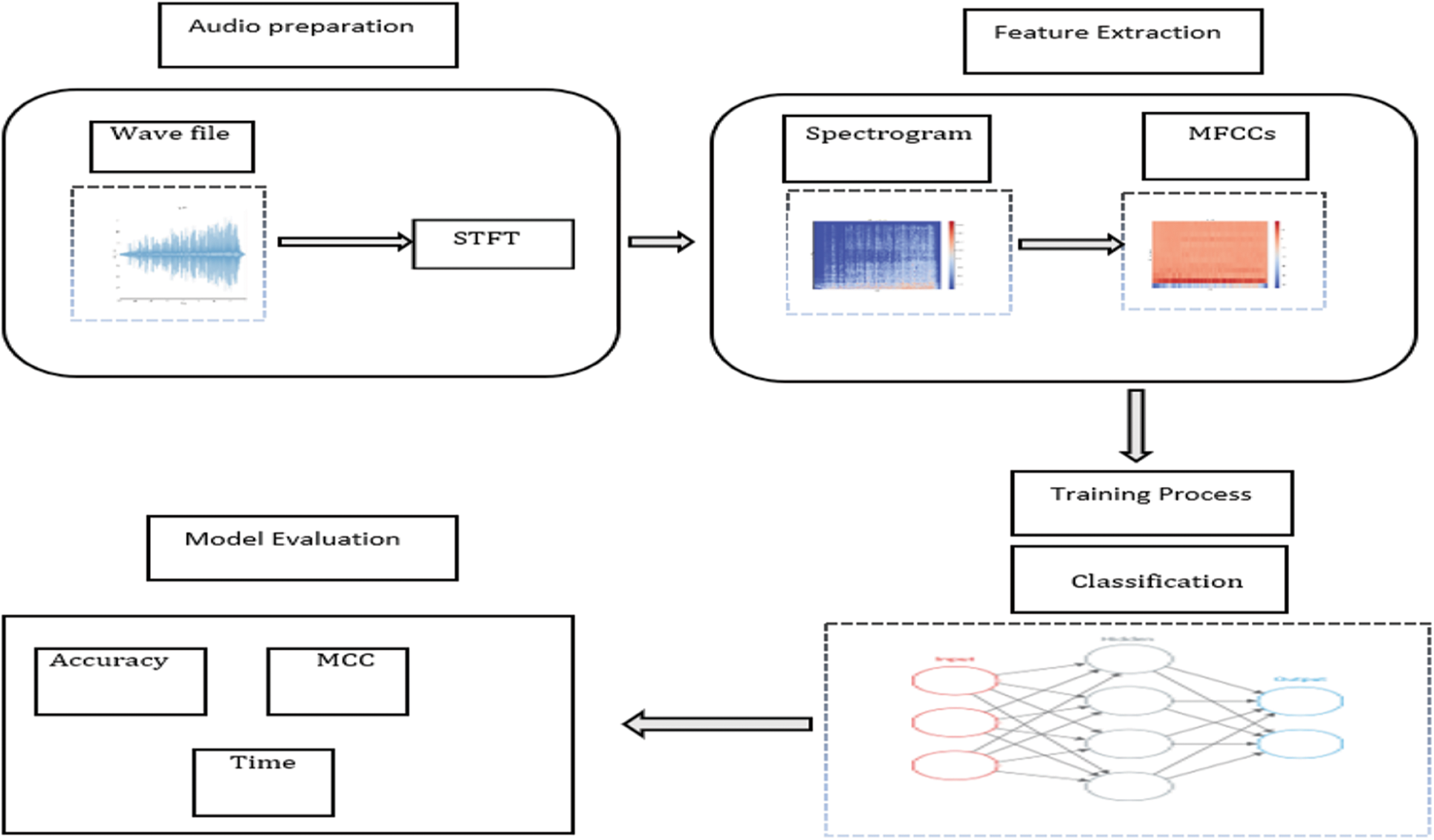
Figure 1: Overall framework
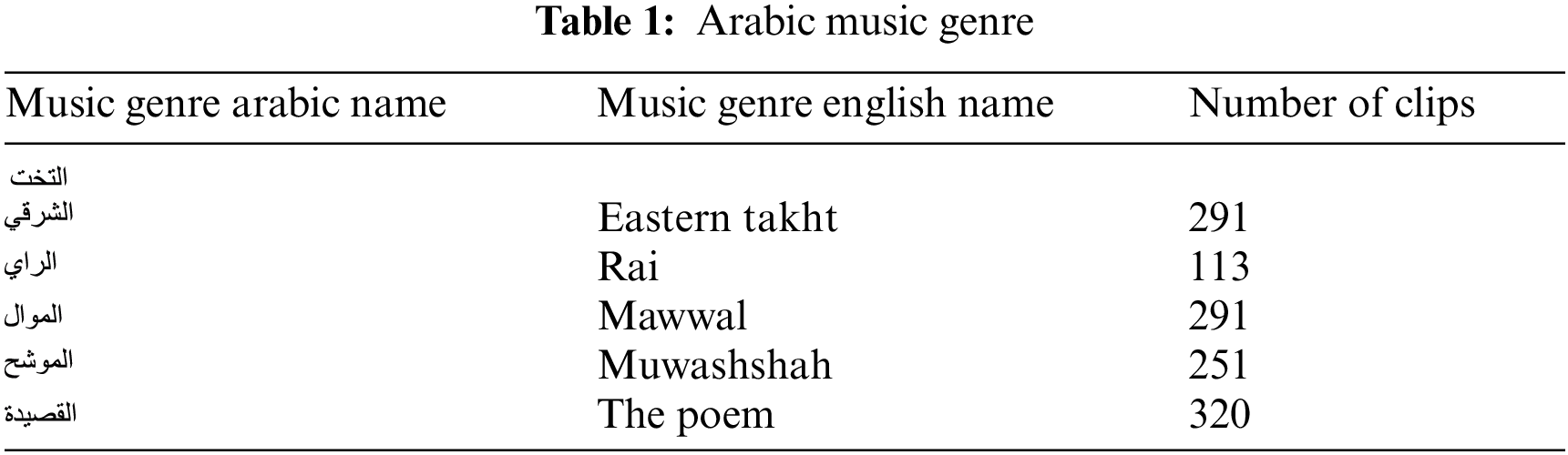
The large corpus of the Arabic Music Genre (AMG) dataset is built by extracting numerous audio clips from YouTube. The dataset consists of five different known genre classes, as presented in Tab. 1. The AMG consists of 1266 audio tracks, each music piece of 30 s long, stored as a 799 MB wav audio file.
The AMG dataset is well-annotated and well-structured of Arabic audio clips. This dataset is available freely for the research community on Arabic MGC on Kaggle under the title “Ar-MGC: Arabic Music Genre Classification Dataset” [34].
The dataset has the following folders:
• Genres original — A collection of 5 genres with 1266 audio files, all are having a length of 30 s.
• Images original — A visual representation for each audio file.
• 1 JSON file — Contains features of the audio files. This JSON file contains three sections:
Mapping-> contains a name of the music genre.
Labels-> which represented as numbers for each genre [0–4].
MFCC-> which represented as a vector with size 13, and contains the features extracted by MFCC.
The methodology implementation starts with WAVs files to convert them into spectrograms. WAVs were initially developed by Microsoft and IBM back in 1991. It is a waveform audio file format, and it is used to store uncompressed recorded sound with high fidelity.
Figs. 2 and 3 show waveforms of two AMG; Muwashshah and the Poem as time on the x-axis and amplitude on the y-axis. In this case, the visual representations for both genres clearly illustrate the difficulty in distinguishing each genre from the other one, so the Genre prediction by visual inspection is not evident.
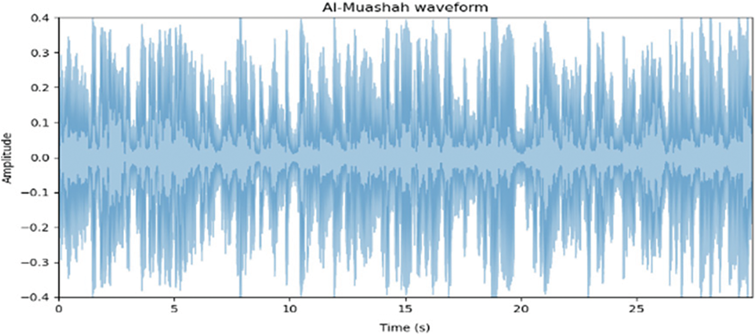
Figure 2: Waveform of muwashshah genre

Figure 3: Waveform of the poem genre
STFT stands for Short Time Fourier Transform. It shows the changes in the frequency content over time by applying a series of windows to the signal using a DFT algorithm, and then all resulting DFTs are placed together in a single graph called a spectrogram, as shown in Fig. 4. In this work, the parameters used to generate the spectrogram are as follows:
• Sampling rate (sr) = 22050
• Window size (n_fft) = 2048
• Hop_size = 512

Figure 4: Spectrogram of the poem genre
MFCCs stands for Mel-Frequency Cepstral Coefficients, introduced in the 1990 s by Davis et al. [35]. It is one of the most popular state-of-the-art feature extraction methods because of its faster extraction technique than other methods such as Perceptual Linear Prediction (PLP) and Linear Prediction Coefficients (LPC). The MFCC summarizes the frequency distribution throughout the window size, allowing for analysis of the sound’s time and frequency characteristics.
In this work, first, the STFT of the audio signal is taken with n_fft= 2048 and hop_size = 512, next, the logarithm of the powers is taken at domain frequencies, then to map the powers onto the Mel-Scale using triangular overlapping windows, and then the final step to apply Discrete Cosine Transform, thereby obtaining the MFCCs, whereas 12656 is many audio features are extracted using the LibROSA package [36].
CNNs are a type of deep neural network that is commonly used in computer vision applications. Furthermore, the uses of CNNs might be extended for any audio analysis applications because the architecture of 2D CNNs can process audio data after MFCC transformation, as it will deal with spectrograms as input. Similarly, as the architecture of 2D CNNs used with image processing tasks, it can also process spectrograms as images due to variations of musical patterns. A spectrogram is a 2D visual representation of the spectrum of audio frequencies over time, which is the convolved input using filters that identify essential characteristics to match the output. Therefore, CNN learns mostly hierarchical features through convolutions. Convolution produces a dot product between the filter and the pixels convolving the entire image as the output of the first convolution layer. Then this features map is sent into the next layer to produce many more features maps until it reaches the end of the network with extremely detailed general information about the image contents. The numbers within the filters are known as weights, and these represent the parameters trained during the training phase. CNNs are composed of convolution layers to learn hierarchical features and an activation function, and a pooling layer between each convolution layer. These activation functions employ the backpropagation approach to calculate the error and then propagate this error across the network, altering the weights of the filters based on this error. Indeed, the most used activation function is known as the Rectified Linear Unit (ReLU) function. Typically, to simplify the network and reduce the number of parameters, pooling layers are another building block of a CNN, and max pooling is the most common operation used in pooling [37].
As explained above, that is the basic form of CNN; accordingly, there have been many different CNN architectures since the pioneering one, which is LeNet5 [12] by LeCun et al., in 1998, next, is AlexNet [38] by Krizhevsky et al., in 2012, the deep learning network applied in the most popular object recognition competition, called ImageNet LSVRC-2010 contest to classify the 1.2 million images into the 1000 different classes. Next, with the progress of the GPUs, is VGG [39] by Simonyan et al. in 2015. Later, ResNet [40] by He et al. in 2016. Nowadays, most state-of-the-art architectures [41] perform similarly and have some specific use cases where they are better. In the following, we detail the most used CNN architectures [42] implemented in this paper, in addition to LSTM [43].
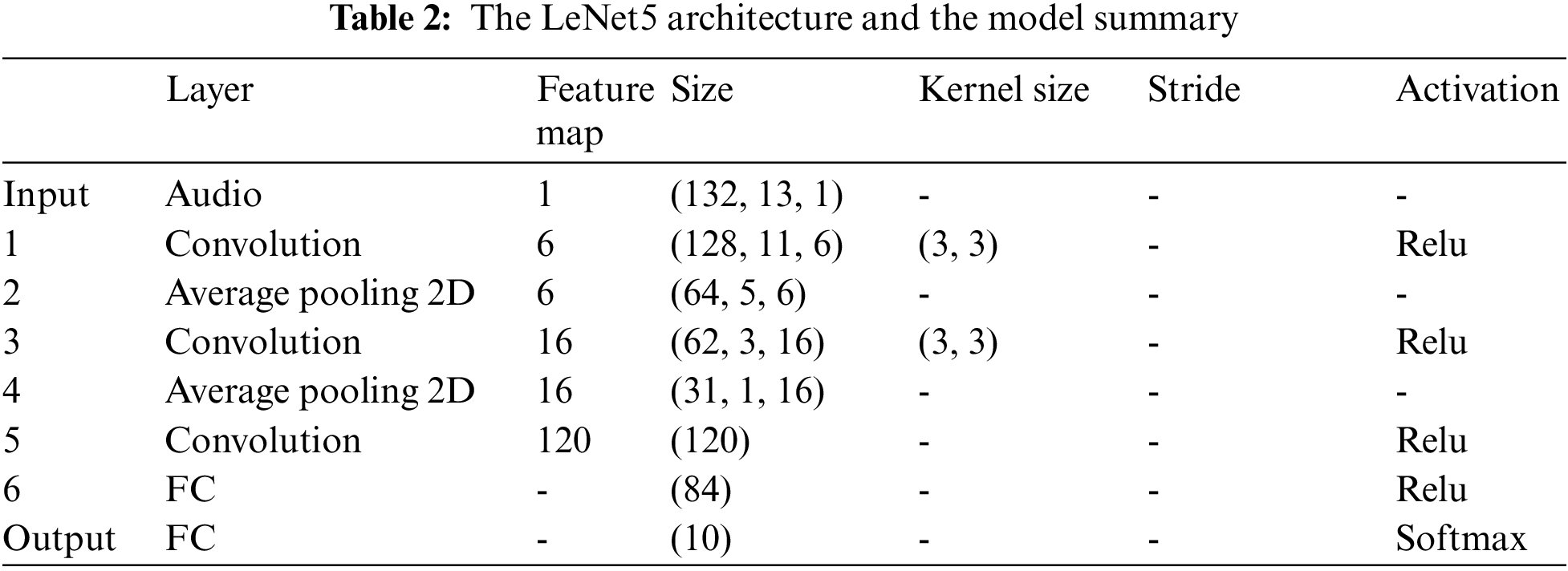
LeNet is the most common class of neural network architectures, as it is one of the earliest deep learning architectures. LeNet5 constitutes of five alternating convolutional and pooling, followed by two fully connected layers in the end. It employs convolution to preserve the spatial orientation of features and average pooling for downsampling of the feature space and ReLU and softmax activation between layers. The summary of the LeNet5 model is shown in Tab. 2. The summary shows the total number of layers, the input size of each layer, the used activation functions employed, and more parameters.
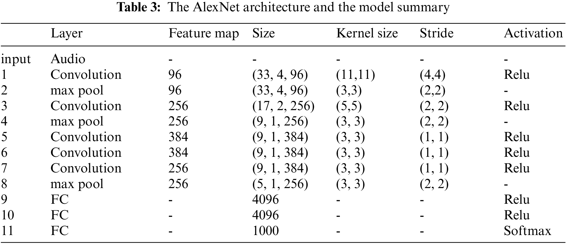
AlexNet was one of the first deep neural networks in the 21st century. It is a deeper version of the LeNet5, which won the most popular object recognition competition, called ImageNet LSVRC-2010 contest, to classify more than one million images into the 1000 different classes. Advancement in computational hardware, GPU, and huge dataset availability aided the network’s success in the competition.
The architecture of AlexNet consists of eight learned layers. It is five convolution layers followed by three fully connected layers. Each convolutional layer has a convolutional filter followed by a nonlinear activation function (ReLU). Between the first and second convolutional layers, max pooling and normalization operations add shift invariance and numerically stabilize learning, respectively. The third, fourth and fifth convolutional layers are connected to one another without any intervening pooling or normalization layers. Tab. 3 shows the summary of the AlexNet model. The summary shows the total number of layers, the input size of each layer, the used activation functions, and more parameters.
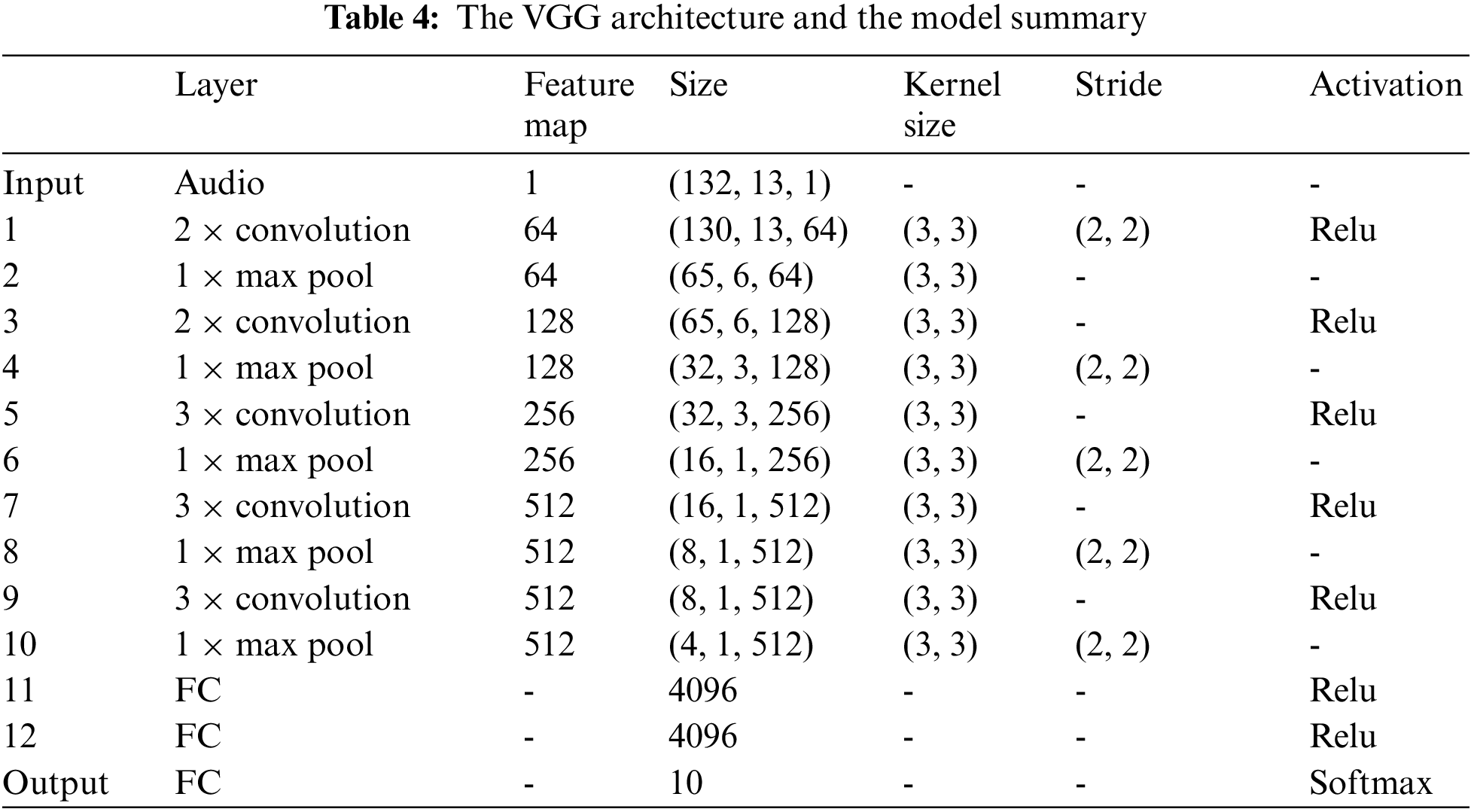
The VGG model was developed in 2014 by the visual geometry group at Oxford to handle another crucial component of convolution architecture design which is depth. VGG would have 11 to 19 layers compared to AlexNet’s eight layers. To this aim, other architectural parameters were fixed. At the same time, depth was gradually increased by adding more convolutional layers, which was possible due to relatively small convolution filters in all layers’ levels. The spectrograms are passed through a stack of convolution layers. The filters have a very small receptive field of 3 cross 3, which is the smallest size required to capture the notions of left-right, up-down, and center. This results in a significant parameter decrease. Spatial pooling is also carried out by five max pooling layers that follow some of the convolutional layers. Tab. 4 summarizes the VGG model. The summary displays the overall number of layers, the input size of each layer, the activation functions employed, and additional parameters.
Typically, previous models to the ResNet have depths of 16 and 30 layers, whereas ResNet could be trained very deep up to a hundred and fifty-two layers in the network. This is 8 times more than that of the VGG nets. ResNet-50 is a CNN that is 50 layers deep using residual connections. As a result, instead of learning unreferenced functions, the layers are reformulated as learning residual functions concerning the layer inputs. Fig. 5. Shows a simple flow chart for RestNet with the residual connection, which is the building block that utilizes skip connections to bypass some layers. There are two primary reasons for adding skip connections: to prevent vanishing gradients and alleviate the Degradation (accuracy saturation) problem. In addition, an extra weight matrix may be employed; these models are known as HighwayNets.

Figure 5: The ResNet flowchart
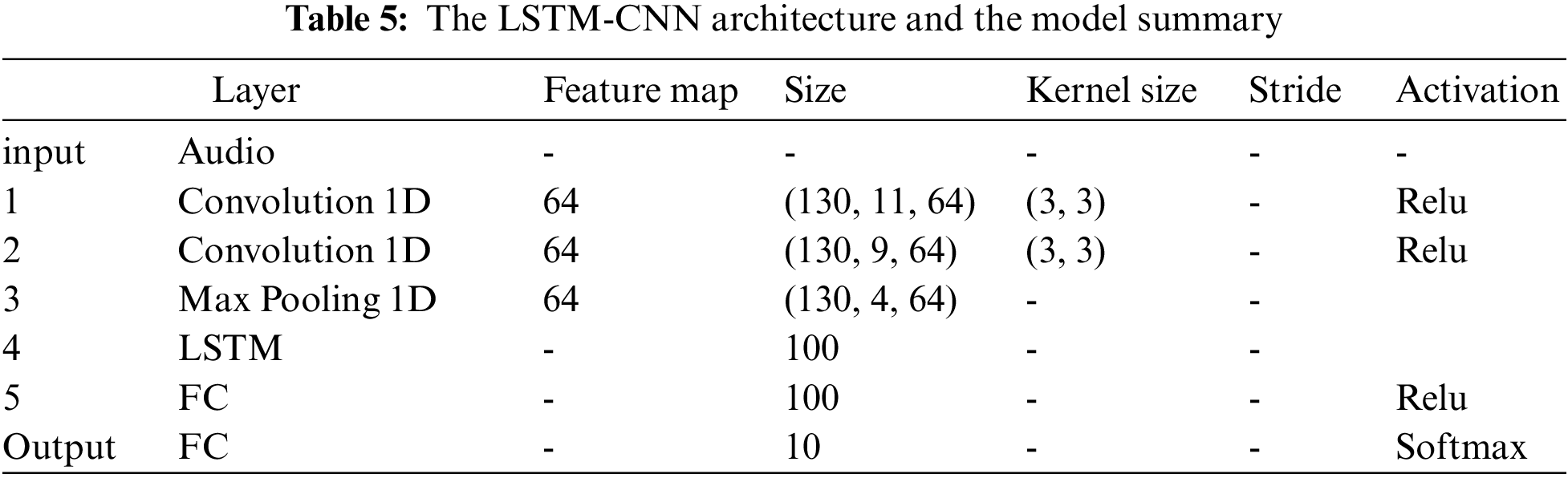
The overall architecture of LSTM-CNN model combines convolutional block and Long Short-Term Memory (LSTM) block to capture spatial features and temporal features within the data, respectively. In the first convolutional block, the input data will be convoluted with a filter map by sliding the kernel window. There is a pooling layer, which is a way of compressing the convoluted data further. Here, the max pooling is used by considering the max from the vector. The second block, LSTM block [43], acts as a sequence to vector, and it is ideal for capturing long-term patterns within the time series data. Finally, the final output layer acts as a fully connected artificial neural network, and SoftMax activation function is used to generate the output. The summary of the LSTM-CNN model is shown in Tab. 5. The summary shows the total number of layers, the input size of each layer, the activation functions employed, and more parameters.
One of the main objectives of this study is to evaluate the performance of all trained models described in Section 3 on our new created dataset; the AMG dataset, which consists of 1266 audio tracks, each track piece of 30 s long, stored as wav audio files at a sampling rate of 22050 Hz. Samples were classified into the following five Arabic musical genres: Eastern Takht, Rai, Muwashshah, the poem, and Mawwal. AMG dataset was split into75% for the training set and 25% for the testing set.
In order to build our approach and evaluate it, the experiment was performed under a GPU server (Kaggle notebook) using Python 3 [44]. MFCC features is computed from audio signals were sent to the deep CNN models for training.
In general, MIR field provides two main parameters for evaluating the system performance: accuracy and Matthew’s correlation coefficient (MCC), in addition to the time required to run the model.
The percentage of correctly classified audio samples is referred to as accuracy [45]. It includes all four possibilities: True Positives (TP), True Negatives (TN), False Positives (FP), and False Negatives (FN). This formula defines the accuracy.
Matthew’s correlation coefficient determines the correlation between true class and predicted class. The higher the correlation between true and predicted values, the better the prediction, and mathematically is defined as
An empirical experiment was performed using different epochs and learning rate parameters to compare CNN model performance. Learning rate controls how quickly or slowly a CNN model learns a problem, and epoch refers to one cycle through the full training dataset. Indeed, it is an art in ML to determine the number of sufficient epochs for a network; hence, three epochs’ values were used (30, 50, 70), and three learning rates were used (0.001, 0.0001, 0.00005). The experimental results show a perfectly configured learning rate, and epochs are 0.00005 and 70, respectively.
The performance of the different CNN models with the learning rate 0.00005 and the different epochs values is summarized in Tab. 6. The best result shows that AlexNet model obtained a 96% test accuracy on the dataset and 95% on MCC within 6.4 s. Figs. 6–8 illustrate the overall performance in terms of Accuracy, MCC and time, respectively. Furthermore, the confusion matrix of AlexNet model shows superior performance with Eastern Takht genre classification reaching an accuracy rate of 99%, as illustrated in Fig. 9.


Figure 6: Performance evaluation of all classifiers on the dataset in terms of accuracy

Figure 7: Performance evaluation of all classifiers on the dataset in terms of MCC

Figure 8: Performance evaluation of all classifiers on the dataset in terms of time

Figure 9: Confusion matrix of AlexNet model
Using the constructed dataset titled “Ar-MGC: Arabic Music Genre Classification Dataset”, we performed a complete empirical comparison of deep CNNs architectures in this study. In the methodology, the audio data was transformed into a spectrogram using STFT. MFCC was applied to extract the audio features, and finally, a classification task was carried out using CNNs.
Comparing the reviewed related works mainly implemented in western MGC using various ML algorithms. AlexNet model obtained higher accuracy on automatic classification between five of the most well-known Arabic music genres: Eastern Takht, Rai, Muwashshah, the poem, and Mawwal.
Many CNNs architectures were explored with their design parameters and evaluation. The results of the experimental evaluation are encouraging to incorporate this work into the mood analysis system on music preferences as music has the potential to impact our brains. This psychological investigation involves EEG analysis.
Funding Statement: The authors received no specific funding for this study.
Conflicts of Interest: The authors declare that they have no conflicts of interest to report regarding the present study.
1. A. Kumar, A. Rajpal and D. Rathore, “Genre classification using feature extraction and deep learning techniques,” in 2018 10th Int. Conf. on Knowledge and Systems Engineering (KSE), Hong Kong, pp. 175–180, 2018. [Google Scholar]
2. T. Li, A. Chan and A. Chun, “Automatic musical pattern feature extraction using convolutional neural network,” in Proc. of the Int. Multi- Conf. of Engineers and Computer Scientists (IMECS), pp. 1–6, 2010. [Google Scholar]
3. U. Bagci and E. Erzin, “Automatic classification of musical genres using inter-genre similarity,” IEEE Signal Processing Letters, vol. 14, no. 8, pp. 521–524, 2007. [Google Scholar]
4. C. McKay and I. Fujinaga, “Automatic music classification and the importance of instrument identification,” in Proc. of the Conf. on Interdisciplinary Musicology, Canada, pp. 1–10, 2005. [Google Scholar]
5. P. Annesi, R. Basili, R. Gitto, A. Moschitti and R. Petitti, “Audio feature engineering for automatic music genre classification,” in Proc. of 8th Int. Conf. on Computer-Assisted Information Retrieval (RIAO), PA, USA, 2007. [Google Scholar]
6. A. Karatana and O. Yildiz, “Music genre classification with machine learning techniques,” in 2017 25th Signal Processing and Communications Applications Conf. (SIU), Antalya, Turkey, pp. 1–4, 2017. [Google Scholar]
7. G. Tzanetakis and P. Cook, “Musical genre classification of audio signals,” IEEE Transactions on Speech and Audio Processing, vol. 10, no. 5, pp. 293–302, 2002. [Google Scholar]
8. K. Chen, S. Gao, Y. Zhu and Q. Sun, “Music genres classification using text categorization method,” in IEEE 8th Workshop on Multimedia Signal Processing, Canada, pp. 221–224, 2006. [Google Scholar]
9. J. Yoon, H. Lim and D. Kim, “Music genre classification using feature subset search,” International Journal of Machine Learning and Computing, vol. 6, no. 2, pp. 134–138, 2016. [Google Scholar]
10. J. Downie, D. Byrd and T. Crawford, “Ten years of ISMIR: Reflections on challenges and opportunities,” in 10th Int. Society for Music Information Retrieval Conf. (ISMIR), Japan, pp. 13–18, 2009. [Google Scholar]
11. A. Khan, A. Sohail, U. Zahoora and A. Qureshi, “A survey of the recent architectures of deep convolutional neural networks,” Artificial Intelligence Review, vol. 53, pp. 5455–5516, 2020. [Google Scholar]
12. Y. LeCun, L. Bottou, Y. Bengio and P. Haffner, “Gradient-based learning applied to document recognition,” in Proceedings of the IEEE, vol. 86, no. 11, pp. 2278–2324, 1998. [Google Scholar]
13. A. Krizhevsky, I. Sutskever and G. Hinton, “ImageNet classification with deep convolutional neural networks,” Communications of the ACM, vol. 60, no. 6, pp. 84–90, 2017. [Google Scholar]
14. K. Simonyan and A. Zisserman, “Very deep convolutional networks for large-scale image recognition,” In ICLR Conference, San Diego, CA, USA, pp. 1–14, 2015. [Google Scholar]
15. B. Sturm, “An analysis of the GTZAN music genre dataset,” in Proc. of the Second Int. ACM Workshop on Music Information Retrieval with User-Centered and Multimodal Strategies (MIRUM’ 12), ACM, NY, USA, pp. 7–12, 2012. [Google Scholar]
16. W. Chai and B. Vercoe, “Folk music classification using hidden markov models,” in Proc. of Int. Conf. on Artificial Intelligence, vol. 6, no. 6, pp. 1–6, 2001. [Google Scholar]
17. C. Xu, N. Maddage and X. Shao, “Automatic music classification and summarization,” IEEE Transactions on Speech and Audio Processing, vol. 13, no. 3, pp. 441–450, 2005. [Google Scholar]
18. A. Girsang, A. Manalu and K. Huang, “Feature selection for musical genre classification using a genetic algorithm, “Advances in Science, Technology and Engineering Systems, vol. 4, no. 2, pp. 162–169, 2019. [Google Scholar]
19. G. Tzanetakis and P. Cook, “MARSYAS: A framework for audio analysis,” Organised Sound, vol. 4, no. 3, pp. 169–175, 2000. [Google Scholar]
20. J. de Sousa, E. Pereira and L. Veloso, “A robust music genre classification approach for global and regional music datasets evaluation,” in IEEE Int. Conf. on Digital Signal Processing (DSP), Beijing, China, pp. 109–113, 2016. [Google Scholar]
21. T. Li and M. Ogihara, “Toward intelligent music information retrieval,” IEEE Transactions on Multimedia, vol. 8, no. 3, pp. 564–574, 2006. [Google Scholar]
22. D. Turnbull and C. Elkan, “Fast recognition of musical genres using rbf networks,” IEEE Transactions on Knowledge and Data Engineering, vol. 17, no. 4, pp. 580–584, 2005. [Google Scholar]
23. J. Bergstra, N. Casagrande, D. Erhan, D. Eck and B. Kegl, “Aggregate features and adaboost for music classification,” Machine Learning, vol. 65, no. 2-3, pp. 473–484, 2006. [Google Scholar]
24. Y. Song and C. Zhang, “Content-based information fusion for semi-supervised music genre classification,” IEEE Transactions on Multimedia, vol. 10, no. 1, pp. 145–152, 2008. [Google Scholar]
25. N. Scaringella, G. Zoia and D. Mlynek, “Automatic genre classification of music content: A survey,” IEEE Signal Processing Magazine, vol. 23, no. 2, pp. 133–141, 2006. [Google Scholar]
26. K. Choi, G. Fazekas and M. Sandler, “Automatic tagging using deep convolutional neural networks,” in Proc. of the 17th Int. Society for Music Information Retrieval Conf. (ISMIR 2016), New York City, USA, pp. 805–811, 2016. [Google Scholar]
27. S. Allamy, and A. Koerich, “1D CNN architectures for music genre classification.,” arXiv preprint arXiv:2105.07302, 2021. [Google Scholar]
28. T. Kim, J. Lee and J. Nam, “Sample-level CNN architectures for music auto-tagging using raw waveforms,” in IEEE Int. Conf. on Acoustics, Speech and Signal Process, Calgary, Alberta, Canada, pp. 366–370, 2018. [Google Scholar]
29. C. Jr, A. Koerich and C. Kaestner, “The latin music database,” in Int. Society for Music Inf Retrieval Conf. Philadelphia, USA, pp. 451–456, 2008. [Google Scholar]
30. M. Defferrard, K. Benzi, P. Vandergheynst and X. Bresson, “FMA: A dataset for music analysis,” in 18th Int. Society for Music Inf Retrieval Conf., Suzhou, China, pp. 316–323, 2017. [Google Scholar]
31. H. Cheng, C. Chang and C. Kuo, “Convolutional neural networks approach for music genre classification,” in 2020 Int. Symposium on Computer, Consumer and Control (IS3C), Taichung, Taiwan, pp. 399–403, 2020. [Google Scholar]
32. C. Sènac, T. Pellegrini, F. Mouret and J. Pinquier, “Music feature maps with convolutional neural networks for music genre classification,” in Int. Workshop on Content-Based Multimedia Indexing (CBMI), Florence, Italy. pp. 1–5, 2017. [Google Scholar]
33. F. Mouret, “Personalized music recommendation based on audio features,” Master Thesis. INP ENSEEIHT, Toulouse, France, 2016. [Google Scholar]
34. A. Atawil, “Ar-MGC: Arabic music genre classification dataset” https://www.kaggle.com/dataset/e551c2960440673a7afcd2ea7ca4c979415e7822e085404c99d939cd85f64077. 2021. [Google Scholar]
35. S. Davis and P. Mermelstein, “Comparison of parametric representations for monosyllabic word recognition in continuously spoken sentences,” IEEE Transaction on Acoustics, Speech, and Signal Processing, vol. 28, no. 4, pp. 1929–1936, 1980. [Google Scholar]
36. McFee, Brian, Colin Raffel, Dawen Liang, Daniel PW Ellis, Matt McVicar, Eric Battenberg, and Oriol Nieto, “Librosa: Audio and music signal analysis in python”. In Proceedings of the 14th Python in Science Conference, pp. 18--25. Austin, Texas, USA, 2015. [Google Scholar]
37. L. Gatys, A. Ecker and M. Bethge, “Image style transfer using convolutional neural networks,” in 2016 IEEE Conf. on Computer Vision and Pattern Recognition (CVPR), Las Vegas, NV, USA, pp. 2414–2423, 2016. [Google Scholar]
38. A. Krizhevsky, I. Sutskever and G. Hinton, “ImageNet classification with deep convolutional neural networks,” in Proceedings of the 25th International Conference on Neural Information Processing Systems, California, USA, vol. 1, pp. 1097–1105, 2012. [Google Scholar]
39. K. Simonyan and A. Zisserman, “Very deep convolutional networks for large-scale image recognition,” in Proc. of the Int. Conf. on Learning Representations, Banff, Canada, 2014. [Google Scholar]
40. K. He, X. Zhang, S. Ren and J. Sun, “Deep residual learning for image recognition,” in Proc. of the IEEE Conf. on Computer Vision and Pattern Recognition, Las Vegas, NV, USA, pp. 770–778, 2016. [Google Scholar]
41. A. Khan, A. Sohail, U. Zahoora and A. Qureshi, “A survey of the recent architectures of deep convolutional neural networks,” Artificial Intelligence Review, vol. 53, no. 8, pp. 5455–5516, 2020. [Google Scholar]
42. A. Tarawneh, A. Hassanat, D. Chetverikov and C. Verma, “Invoice classification using deep features and machine learning techniques,” in 2019 IEEE Jordan International Joint Conference on Electrical Engineering and Information Technology (JEEIT), Amman, Jordan, pp. 855–859, 2019. [Google Scholar]
43. S. Hochreiter and J. Schmidhuber, “Long short-term memory,” Neural Computation, pp. 1735–1780, 1997. [Google Scholar]
44. https://www.python.org/downloads/release/python-395/. 2021. [Google Scholar]
45. L. Almazaydeh, K. Elleithy, M. Faezipour and A. Abushakra, “Apnea detection based on respiratory signal classification,” Procedia Computer Science, vol. 21, pp. 310–316, 2013. [Google Scholar]
 | This work is licensed under a Creative Commons Attribution 4.0 International License, which permits unrestricted use, distribution, and reproduction in any medium, provided the original work is properly cited. |