DOI:10.32604/cmc.2022.025692
| Computers, Materials & Continua DOI:10.32604/cmc.2022.025692 | |
| Article |
Cervical Cancer Classification Using Combined Machine Learning and Deep Learning Approach
1Department of Biomedical Engineering, Jordan University of Science and Technology, Irbid, 22110, Jordan
2Department of Biomedical Systems and Informatics Engineering, Yarmouk University 556, Irbid, 21163, Jordan
3Faculty of Electrical Engineering Technology, Campus Pauh Putra, Universiti Malaysia Perlis, 02000, Arau, Perlis, Malaysia
4Advanced Computing, Centre of Excellence (CoE), Universiti Malaysia Perlis (UniMAP), 02000, Arau, Perlis, Malaysia
5The Institute of Biomedical Technology, King Hussein Medical Center, Royal Jordanian Medical Service, Amman, 11855, Jordan
6Department of Computer Engineering, Yarmouk University, Irbid, 21163, Jordan
*Corresponding Author: Wan Azani Mustafa. Email: wanazani@unimap.edu.my
Received: 01 December 2021; Accepted: 02 March 2022
Abstract: Cervical cancer is screened by pap smear methodology for detection and classification purposes. Pap smear images of the cervical region are employed to detect and classify the abnormality of cervical tissues. In this paper, we proposed the first system that it ables to classify the pap smear images into a seven classes problem. Pap smear images are exploited to design a computer-aided diagnoses system to classify the abnormality in cervical images cells. Automated features that have been extracted using ResNet101 are employed to discriminate seven classes of images in Support Vector Machine (SVM) classifier. The success of this proposed system in distinguishing between the levels of normal cases with 100% accuracy and 100% sensitivity. On top of that, it can distinguish between normal and abnormal cases with an accuracy of 100%. The high level of abnormality is then studied and classified with a high accuracy. On the other hand, the low level of abnormality is studied separately and classified into two classes, mild and moderate dysplasia, with ∼ 92% accuracy. The proposed system is a built-in cascading manner with five models of polynomial (SVM) classifier. The overall accuracy in training for all cases is 100%, while the overall test for all seven classes is around 92% in the test phase and overall accuracy reaches 97.3%. The proposed system facilitates the process of detection and classification of cervical cells in pap smear images and leads to early diagnosis of cervical cancer, which may lead to an increase in the survival rate in women.
Keywords: Classification; deep learning; machine learning; pap smear images; resnet101; support vector machines
Cervical cancer is a disease in which cells in a woman’s cervix develop uncontrollably. This cancer is named after the initial site of origin, even when it afterwards spreads towards other organs. The vagina (birth canal) and the upper part of the uterus are connected by the cervix. Meanwhile, in the uterus (also known as the womb), the baby develops during pregnancy. Cervical cancer is a disease that affects all women. It is more prevalent in women aged 30 and up. Cervical cancer is caused by long-term infection with the Human papillomavirus (HPV), a sexually transmitted disease. Most sexually active people will contract HPV, but only a small number of women will develop cervical cancer, which is affected by other factors [1]. The segmented Pap Smear image is one of the detection techniques with several different approaches. The detection of cervical cancer cells is required before classification. The solution involved comparing the dissimilar performance of existing techniques using various existing detection approaches. Improving the precision of system performance is required to develop a new method [2]. Cervical cancer classification methods were thoroughly researched. This resulted in a deeper examination of database attributes, cervical cancer categories, classification techniques, and system performance [3].
Classification of images is the primary domain in which deep neural networks are most effective in medical image analysis. If a disease occurs, it can be determined by using the image classification, which accepts images as input to generate output classifications. Many different ideas of classification mechanisms have been proposed to identify cervical cancer diagnoses. Current research appears to validate the view of the schematic representation of the used and proposed ordinal losses in Fig. 1. This study proposed losses (CO, CO2, and HO2). The Herlev Dataset was used in this study.
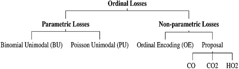
Figure 1: Schematic representation of the used and proposed ordinal losses [4]
In article by Albuquerque et al. [4], the researcher has proposed a new non-parametric loss for the multi-class Pap smear cell classification. This proposed method was based on a convolutional neural network. This Non-parametric loss outperformed parametric losses when compared to ordinal deep learning architectures on cervical cancer data. According to the study findings, this new loss can compete with current results and is more flexible than existing deep ordinal classification methods, which impose unimodality on the probabilities. However, the proposed loss involves two new hyper-parameters to be calculated, where other ordinal classification applications may be able to use the proposed loss. As a result, results are still below 75.6% accurate. It is fascinating to compare with another study by Gibboni [5]. This study, however, uses a different database from the TissueNet: Detect Lesions in Cervical Biopsies, which contains thousands of “whole slide images” WSIs of uterine cervical tissue from medical centers. Four classes of WSIs are recognized: benign (class 0), low malignant potential (class 1), high malignant potential (class 2), and invasive cancer (class 3). Self-supervised training with Multiple Instance Learning (MIL) is used by this researcher to classify WSIs using only coarse-grained image-level labeling. This is the first time a self-supervised learning-based pre-trained model has been implemented for cervical cancer entire slide images classification. Self-supervision is implemented very well in WSIs classification, according to this research. The researcher compares the consequence of the proposed pre-trained model to the ResNet18 model pre-trained on ImageNet to assess its effectiveness. Initially, the accuracy increases as the number of clusters increases, but as the number of clusters increases to 10, the accuracy decreases [6].
The database used in this study is derived from the CRIC Searchable Image Database’s cervical cell classification collection [7] (available online at https://database.cric.com.br, accessed on September 2021). The Center for Recognition and Inspection of Cells created these cervical cell images for this dataset (CRIC). The ensemble methodology’s primary objective is to assess several classification models and integrate them to produce a classifier that overrides them individually. After each architecture created its predictions, we combined the three top architectures in terms of recall values to form an ensemble approach. In the event of a tie, the decision of the architecture with the highest recall value took precedence [8]. The proposed ensemble in [8] is depicted in Fig. 2.
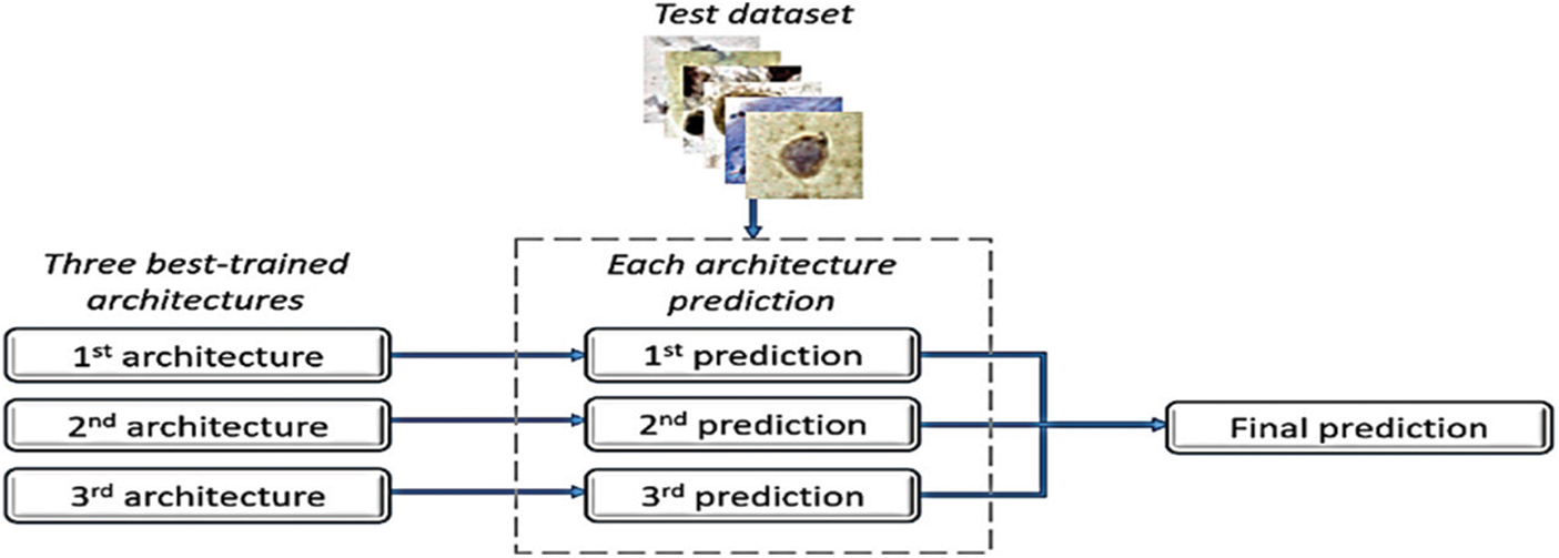
Figure 2: Ensemble method [8]
Furthermore, a paper by Diniz et al. [9] has shown that a selection of the SIPaKMeD cervical cell image dataset from the 2018 International Conference on Image Processing demonstrates the effectiveness and feasibility of the proposed method. Fig. 3 shows the proposed method of cervical cell image framework model by Diniz et al. [9]. A CNN model pre-trained in the cervical cell classification model initially extracts the features of cell images. Then, K-means clustering is applied to these CNN features, allowing the cluster centers to be obtained. Given that the clusters are possible to be significantly correlated, the graph of clustering centroid correlation is constructed based on its inherent resemblances. The constructed graph allows for further exploration of the potential relationships among image data. Following that, two-layer GCN is used to learn over the graph structure and node features to produce relation-aware node features. Since linear projection, a cross-entropy loss is used to train the entire network. The goal of the Graph Convolutional Network (GCN) is to discover the relation-aware image features of nodes by propagating the graph’s inherent structure information. In contrast to CNN-based approaches that perform convolution on local Euclidean structure, GCN generalizes convolution operation to non-Euclidean data (e.g., a graph). Furthermore, it undertakes convolution on neighboring nodes’ spectral graphs and updates the feature representation of each node to include graph structure during training [10].
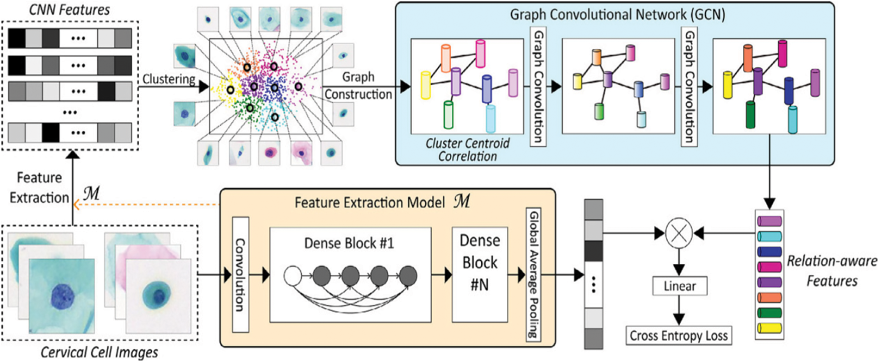
Figure 3: Classification framework of our method for cervical cell images [9]
Many researchers have carried out their experiments by utilizing the facilities in artificial intelligence techniques. This includes Shi et al. [11], who proposed a classification model for cervical images based on CNN structure, achieving high accuracy in discriminating between two classes, reaching 99.5% and 91.2% for seven classes. On the other hand, Ghoneim [12] utilized the benefits of deep transfer learning based on snapshot ensemble (TLSE), which is a new strategy in training. Their highest accuracy reached 65.56% for seven classes. In addition, Chen [13] used the deep learning method besides transfer learning for pretrained convolutional neural networks. They obtained the highest accuracy, but their proposed method suffered from requiring high computation time. Classification of a single patch requires 3.5 s, which is too slow in a clinical setting. Moreover, Zhang et al. [14] enhanced the images using a local adaptive histogram. Then, cell segmentation was performed through a Trainable Weka Segmentation classifier. The feature selection step is achieved then the classification is performed using a fuzzy c-means algorithm. Their classes are just normal and abnormal cervical images. On top of that, William [15] classified pap smear images into normal and abnormal by ensemble classifier with SVM, multilayer perceptron classifier and random forest, that takes high computation time beside it is focused on two classes only.
This paper proposed an automatic system based on deep graphical features extracted by ResNet101 to classify cervical cancer images. The presented method is focused on the utilization of automated features extraction besides on selecting the most important features to distinguish between seven classes of cervical cancer from pap smear images using Support Vector Machine classifier (SVM). The novelty of this work is the higher performance achieved by the proposed system, which makes it dependable software and can be covered all types of cervical abnormalities. The proposed method can be used to detect the type of cancer early, leading to an increase in women’s survival rate. The performance of the proposed work is tested and compared with previous studies. The rest of the paper reviews some of the conventional methods of cervical cancer detection, the methodologies of the proposed method, and their results. The last section concludes the proposed work.
The proposed recognition approach consists of four main stages: the first stage is to load and resize the whole dataset beside increase its number by augmented it ; the second stage is utilizing CNN to extract the deep features using ResNet101; that is done by splitting the dataset into training and testing sub-datasets; the third stage employing features reduction algorithm; Principal Component Analysis to extract the most significant graphical features, that will reduce the computation time beside to enhance the performance of next stage. the fourth stage training and validate the proposed multi-stage cascaded SVM training and testing datasets, and finally display the results. The following subsections will discuss in detail all used materials and methods.
The study is conducted on the Herlev Pap Smear dataset that is consisted of 917 cell images, and each one contains one single nucleus. The dataset was collected by Herlev University Hospital (Denmark) and the Technical University of Denmark [4]. These cervical cell images are collected manually, which are then annotated into seven classes by skilled cyto-technicians. The distribution of cervical images is presented in Tab. 1. Samples of normal and abnormal classes are shown in Figs. 3–5, respectively.
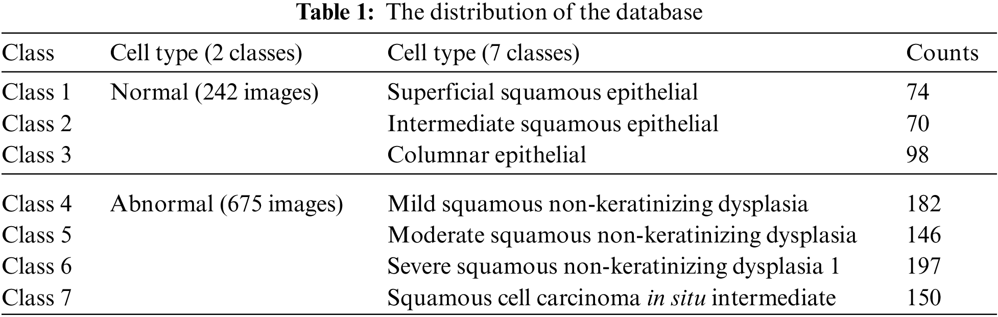
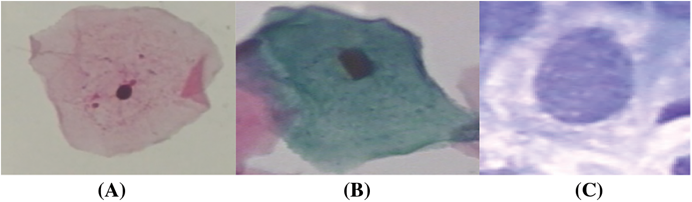
Figure 4: Normal classes cervical images; (a) superficial, (b) intermediate, (c) columnar
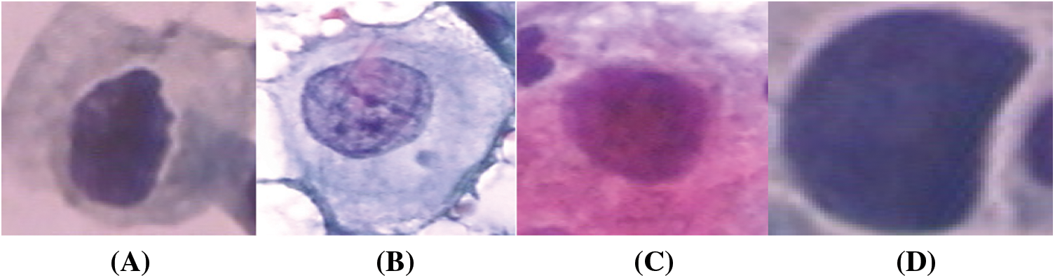
Figure 5: Abnormal classes cervical images; (a) mild, (b) moderate, (c) Severe, (d) carcinoma in situ
All the images in the dataset were utilized are resized to 224 × 224 × 3 pixel as the use ResNet model requires, and neither low-quality nor low-resolution images were excluded. Also, to build a balanced dataset, a set of pre-processing options for images are applied rotation by 45 degrees, reflection in the left-right direction, reflection in the top-bottom direction, Uniform (isotropic) scaling.
Deep Learning (DL) is part of Machine Learning (ML) which is a subfield of Artificial Intelligence (AI). Deep learning is a state-of-the-art technology that is bioinspired by the neural connections of the human brain [16]. Deep Learning methods are representation learning methods, and they gain knowledge from the input data. They learn from experience and do not require explicit programming by engineers. The availability of huge datasets and the massive computing power contributed to its widespread applicability. Contemporary Deep Learning (DL) methods have drawn wide attention because of their various commercial applications. Deep Learning techniques are very popular nowadays and have been used in different domains to solve a broad range of complex problems like Computer Vision, image processing, speech recognition, natural language processing, self-driving cars, and board games [17,18]. In addition, the performance of those techniques exceeded that of conventional methods, and their performance has even surpassed that of a human expert in carrying out some specific tasks. Deep learning uses a dense Artificial Neural Network (ANN) with lots of neurons, synapses, and multilayers coupled together with weighted connections and hence the term “deep”. A typical Deep Learning (DL) algorithm learns and improves by itself. It is trained using huge datasets with millions of data points, and learning can be unsupervised, semi-supervised, or supervised. Unlike traditional methods and techniques, the performance of the deep learning algorithm improves as the size of the dataset increases. In a deep architecture, the first layer extracts low-level features, whereas higher layers recognize more complex and abstract features. For example, the first layer might extract pixels. On the other hand, the second layer might identify edges, while the third layer might distinguish a group of edges or a motif. Also, higher layers might diagnose that a particular image contains a disease. Convolutional Neural Networks (CNN) and Recurrent Neural Networks (RNN) are the most prominent Deep Learning (DL) algorithms [19,20].
Convolutional Neural Networks are the most dominant, capable, and widely used architecture, particularly in the field of computer vision. A Convolutional Neural Network (CNN) is a hierarchical multilayered neural network that takes multidimensional arrays as input and is based on the noncognition architecture developed in 1983 [21,22]. The only difference is that a CNN is self-organized using supervised learning while a noncognition was self-organized by unsupervised learning. A CNN can automatically extract features from the input image, which eliminates the need for manual feature extraction. A typical CNN is made of multiple stages where each stage is comprised of alternating convolutional and pooling layers. The convolutional layers identify local features, and the pooling layer groups similar features together [23]. When the network trains on a set of images, it learns those images, extracts the underlying features, and can eventually perform generalization to decide or make a prediction on unseen data. To eliminate the need for long training hours and immense computing power, pretrained CNNs can be used to perform classification tasks directly. Alternatively, they can be used as a feature extractor followed by a generic classifier. To solve complex tasks and to improve the recognition accuracy, it is recommended to add more layers or to use deeper neural networks. Researchers noticed that adding more layers to the neural network did not improve performance. Instead, it causes the accuracy to improve temporarily, and then it saturates before it eventually degrades. Here ResNet comes to the rescue and helps address the problem [24].
Residual Networks (ResNet) was introduced in 2015 by researchers at Microsoft [25]. They won the 2015 ILSVRC classification contest, among other competitions. It is an extremely deep residual learning framework that uses a Convolutional Neural Network (CNN). It has a 60 × 60 input layer size, 2 × 1 output layer size, 33 residual blocks and can be applied to solve vision and non-vision recognition problems. Depending on the number of layers the model uses, there are multiple versions of the ResNet framework, specifically ResNet18, ResNet50, ResNet101, and ResNet152. The model is pretrained using 1.28 million images, validated using 50 k images from the ImageNet dataset that has 1000 categories [26]. Since model training is a time-consuming task, transfer learning takes advantage of the excellent generalization capability of the ResNet101 model. Therefore, transfer learning uses fewer data to train the models, is less expensive, and is not as time-consuming.
When training “plain” networks, the observation is that as the number of layers increases, the training accuracy saturates then it worsens quickly [27,28]. To address the vanishing gradient problem [29,30], the ResNet utilizes a feedforward neural network with bypass connections avoiding one or more weight layers to perform identity mappings. The output is eventually fused with the output of the stacked layers, as shown in Fig. 1. Unlike regular networks that experience high training errors when the model depth increases, the extremely deep ResNet is easy to optimize. In addition, the accuracy of the ResNet increases as the network depth increases. Finally, ResNet can be easily realized using publicly available libraries and is trained with Stochastic Gradient Descent (SGD) and backpropagation [31].
3.4 Principal Component Analysis (PCA)
Sometimes at the surface, the data seems scattered but using some advanced data mining techniques can reveal some interesting trends. Data scientists believe that there is a lot of information and knowledge that can be gained from digging deep into the data. Developed in 1933 [32], Principal Component Analysis (PCA), also known as the Hotelling transformation, is an old, simple statistical technique that transforms the data from a higher dimension to a lower dimension in hopes of a better understanding of the data. Principal Component Analysis (PCA) is used for dimensionality reduction, data compression, and data visualization. In the dimensionality reduction case, it helps simplify the problem by reducing the number of features dramatically. If the number of features in the original dataset is p, the number of features in the new dataset is q where q << p. Since the new dimension is smaller in size when compared to the original dimension, some information will be lost. PCA can help identify the variables hiding deep in the data. The Scree plot can help prioritize that hidden variable according to the fraction of the total information they retain to identify the principal components. The principal components are uncorrelated, and they are a linear combination of the original data. Two or three of the principal components might account for 90% of the original signal [33–36].
Principal Component Analysis (PCA) is a tool that has found many field applications from neuroscience to quantitative finance. Multiple researchers [37–39] have used Principal Component Analysis (PCA) to identify and classify cervical cancer. Cervical cancer is a serious disease that affects the cervix tissues; however, the disease is 100% curable if detected at an early stage. The problem is that cervical cancer detection can be expensive and time-consuming. Researchers have mainly used Principal Component Analysis (PCA) to help select the risk and clinical features that can be used to identify cervical cancer. They tried to reduce the number of features without losing the clinical information to process the data efficiently and effectively. Most studies tried to simplify the cervical cancer identification and classification problem by eliminating the irrelevant features without affecting cancer identification accuracy. Such work will hopefully lay the ground for building accurate systems that can detect cancer quickly and cost-effectively, thus increasing the women’s survival rate.
Experimentation or analysis is performed to determine the priorities since different states or experiment data have different priorities. For this proposed work, their priorities from high to low are denoted as the Abnormal-Normal category, the High/Low-Normal category, Severe Dysplasia-Carcinoma in-situ category, Mild Dysplasia-Moderate dysplasia category, and Superficial-Intermediate-Columnar category, thus five categories. Because there are five categories, thus there are M-1 levels classifiers; in this case, four levels classifiers. Then the formers (s = 1, 2, . . ., M − 1) levels, in this case, Abnormal-Normal levels classifier find out the corresponding Normal category together, and the (M −1) levels classifiers or four levels classifier is designed using the rest two categories of High/Low and Normal which are not recognized by the former (M − 2) levels or three levels classifier. The design of 4-th (s = 1, 2, . . ., M − 1) level based on feature selection is given as follows:
Let s be 3, the (M − s + 1) categories, that is (5−3 + 1) = 3 categories which cannot be recognized by the former s − 1 levels, that is (3−1) = 2 levels are denoted as {Vi1, Vi2, . . . , Vi(M−s+1)} and the many-to-one binary classifier is denoted by Ʌ (M−s + 1)k (k = 1, 2, . . . , M − s + 1). One category is
These two functions priorities are schemed from high to low, which means if and only if (1) attain the max value as clear in Eq. (1), then min q is to be considered as clear in Eq. (2). Based on (1), classification is performed with the class with the highest classification precision during each level. The concept is when each level attained the highest classification precision and the smallest size of feature subset. Then, the serial SVM garners the highest classification precision and the smallest size of feature subset for the classifier model. Thus, the s-th level is designed to reach the highest classification precision and the least number of feature subsets. The samples are separated into two parts; training and determining the least number of features during the feature subset selection process and classifiers construction purposed to evaluate the selected features [40].
For the classification of M, also meant for five categories, Fig. 6 illustrates the proposed framework of serial and cascading SVM classifier. The SVM binary classifier is used as the base classifier, whereas the SVM multiclass classifier is used for non-binary cases. When samples are input to the serial and cascading SVM classifier, the first category can be recognized by SVM Model 1, while the second is recognized by SVM Model 2. Moreover, the third is SVM Model 3, the fourth is SVM Model 4, and lastly, SVM Model 5. Logically, the (M-2)-th category or third category is recognized by the former (M − 2) SVM classifiers or called SVM Model 3, and the categories (M − 1)-th or fourth category and M-th or fifth category can be recognized by all five SVM classifiers. Unlike the traditional cascade classifiers’ adding predictions of the level to the next level, the cascade model that we proposed classifies the class with the highest classification precision after each level. Here, the number of classes is reduced continuously via serial and cascading SVM models. Each categories’ separability will not affect classifiers of each level simultaneously because they are cascaded, which makes the model more convenient to dig features’ classification potential.
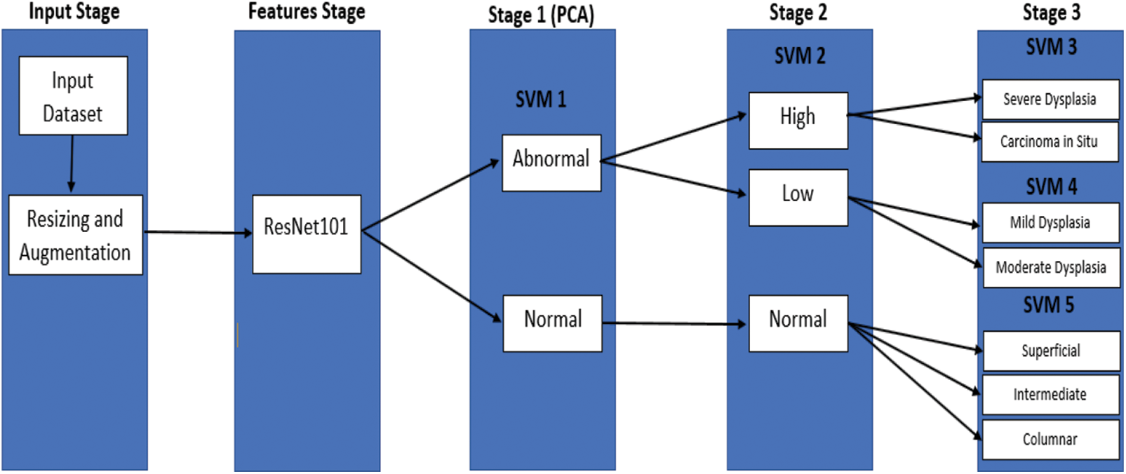
Figure 6: The proposed model
Five serial SVM models are built in MATLAB® in three stages to classify seven cervical cancer images. Tab. 2 illustrates the classification results in terms of accuracy. The training accuracy is 100% in all classes and stages, whereas test accuracy is high in all classes. Four statistical indices, namely true positive (TP), false positive (FP), false negative (FN), and true negative (TN), are computed. Consequently, the Accuracy, Sensitivity, and specificity, the F1 score is calculated [41–43].
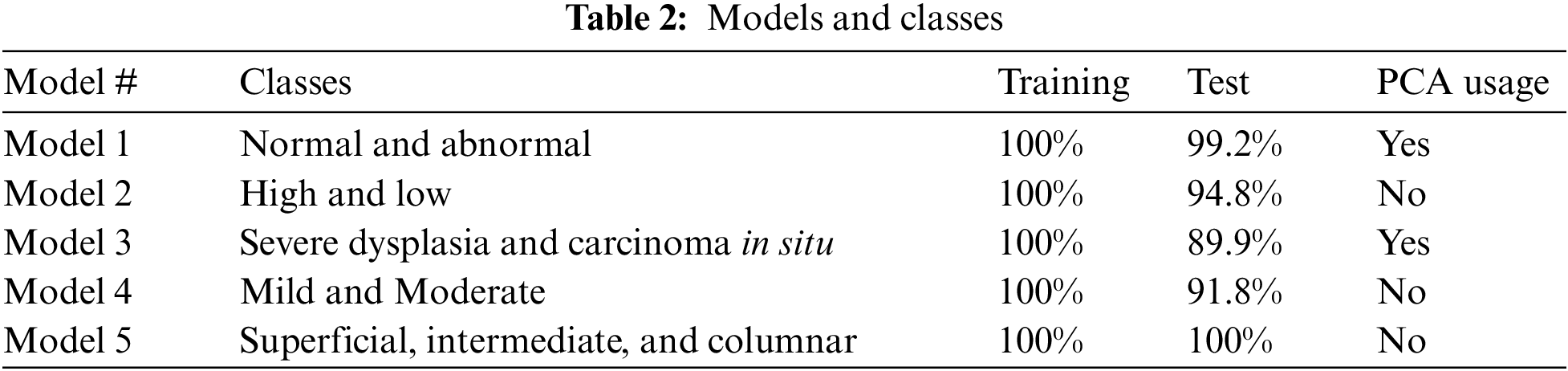
The highest test accuracy, 99.2%, is obtained in terms of distinguishing between normal and abnormal images by utilizing PCA. The testing accuracy in High and Low abnormal cases is 94.8%. In Model 2, all extracted features are exploited to obtain a better class separately. Nevertheless, the highest class is classified into two classes: severe dysplasia and carcinoma in situ with 89.9%. In this stage, all features are employed due to the high similarity between these two types of images. On top of that, the low level is proceeded to discriminate between mild and moderate classes with an accuracy of 91.8%. SVM model 5 is exploited to discriminate between normal cases into superficial, intermediate, and columnar with 100% accuracy for both training and test. The overall data after augmentation is 1341 images, where 30% of them are taken as test data. The number of misclassified images is 34 in the test case, whereas it is zero in the training phase. The overall accuracy for seven classes in the test case is 91.4%. However, the overall accuracy for both phases, test and train, is 97.5%. Tab. 2 illustrates the models that have been built beside the classes, accuracy in training and test, and the usage of PCA or not.
The decision in using PCA or not is based on obtaining the best accuracy and the available automated features that are suitable, or there are redundant features as is clear in stage 1 and stage 3 of the obtained models. The precision, sensitivity, F1-score, and AUC are computed for each model separately. Tab. 3 illustrates the results of each model. While Figs. 7–10, and Fig. 11 show the testing confusion matrix for each SVM model.
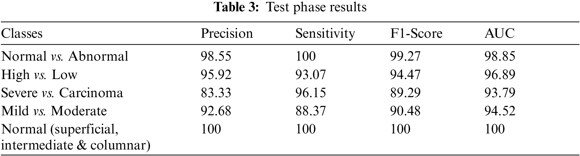
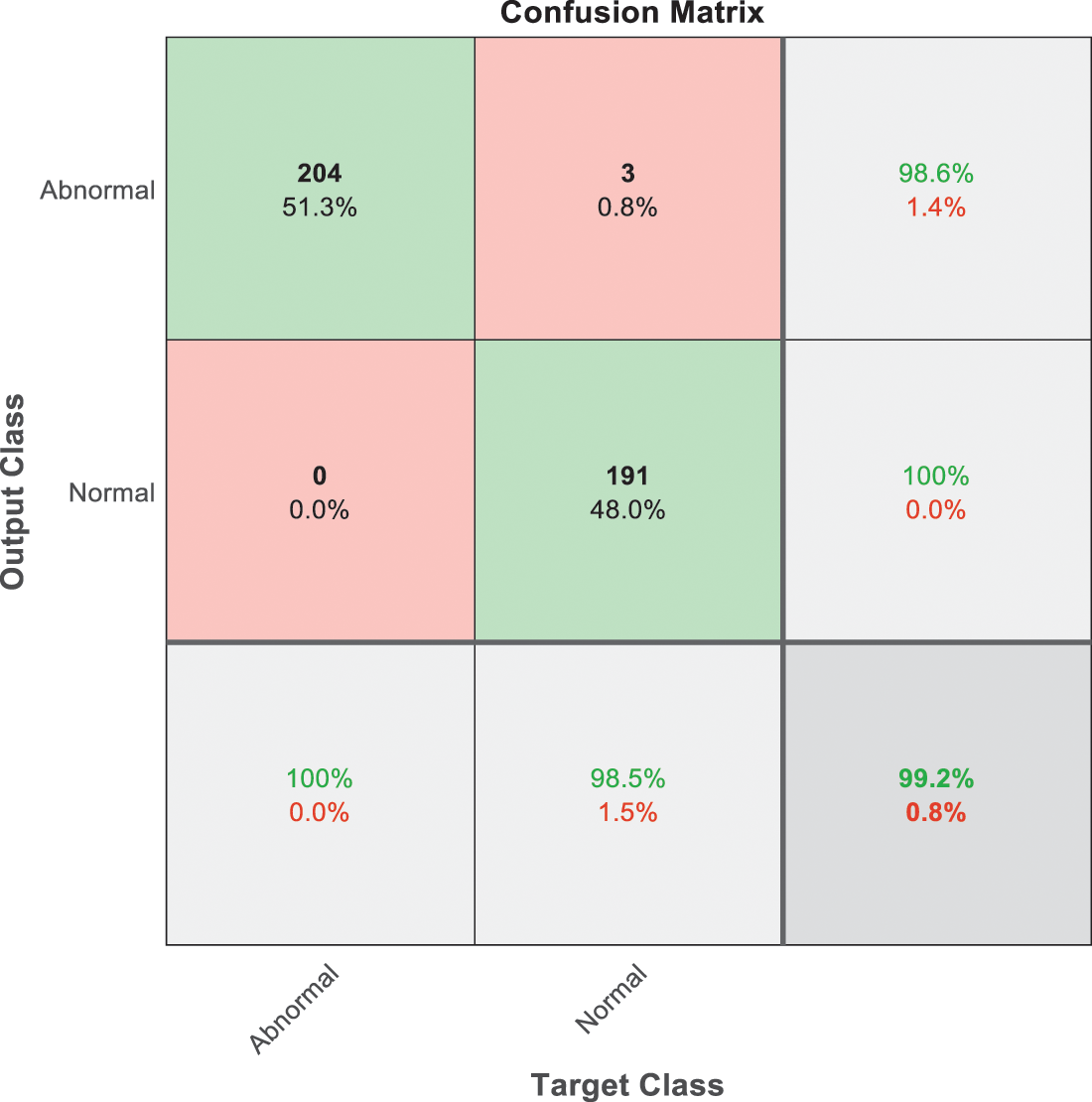
Figure 7: SVM 1 testing confusion matrix
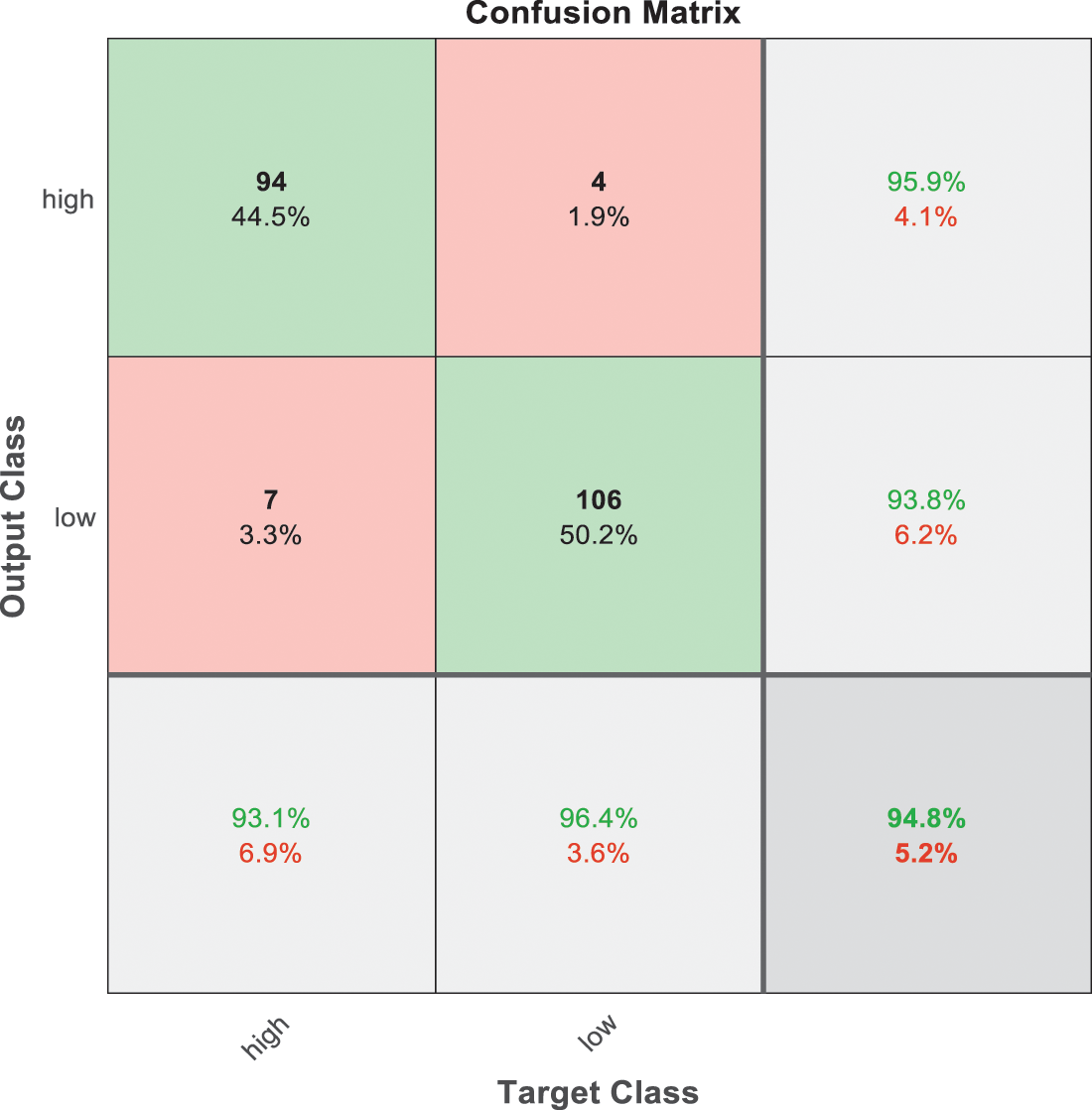
Figure 8: SVM 2 testing confusion matrix
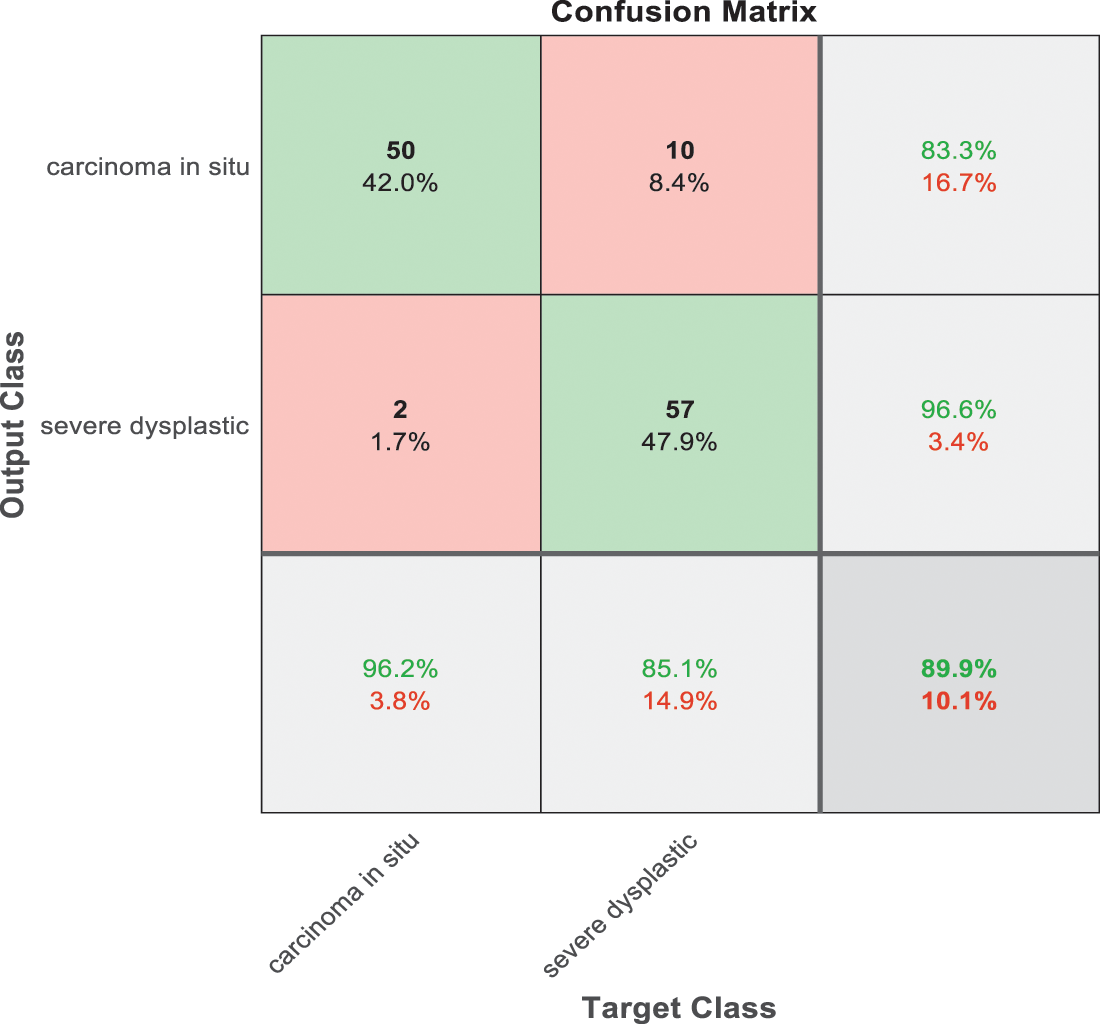
Figure 9: SVM 3 testing confusion matrix
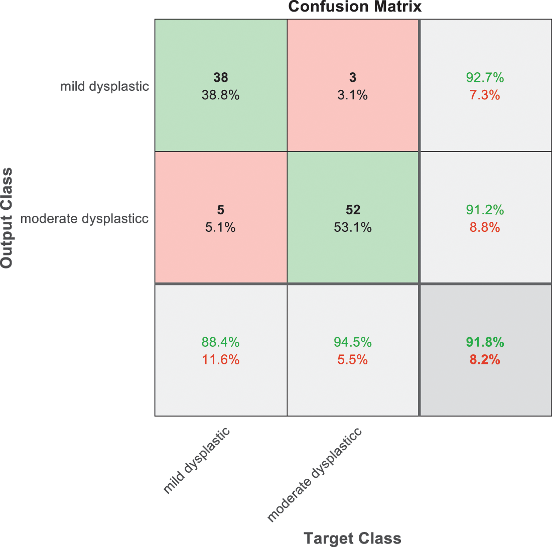
Figure 10: SVM 4 testing confusion matrix
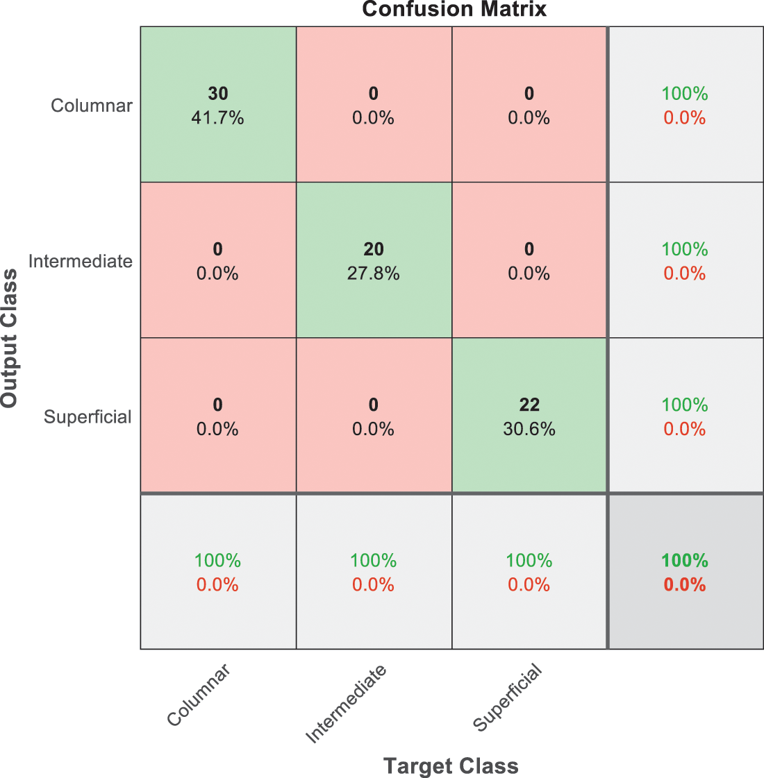
Figure 11: SVM 5 testing confusion matrix
Fig. 7 is demonstrated the results for model 1 which is deploy for distinguishing between normal and abnormal biopsies images. On the other hand, Fig. 8 is illustrated the results of model 2 to discriminate between high and low levels of abnormalness biopsies.
Fig. 9 is exploited to show the results that have been obtained from model 3 for classify high level abnormal biopsies into severe and carcinoma with accuracy 89.9%. Whereas Fig. 10 is clarified the results of model 4 to distinguish between mild and moderate low level abnormalness with accuracy 91.8%.
The last confusion matrix in Fig. 11 presents the results of model 5 which is devoted for classifying the normal biopsies into 3 classes: columnar, Intermediate, and superficial with accuracy 100%. The Receiver Operating Characteristics for all SVM models are clear in Figs. 12, 13, 14, 15, which illustrates the relationship between false-positive rate vs. true positive rate as shown in figures below the high level of TPR that yields a high value for AUC. Fig. 12 is ROC curve for model 1 which illustrates high true positive rate. The same is for model 2 which is illustrated in Fig. 13. Also, Fig. 14 describes the ROC curve for model 3. It is clear that it has a high TPR. Finally, the same for Fig. 15 It shows the ROC for model 4.
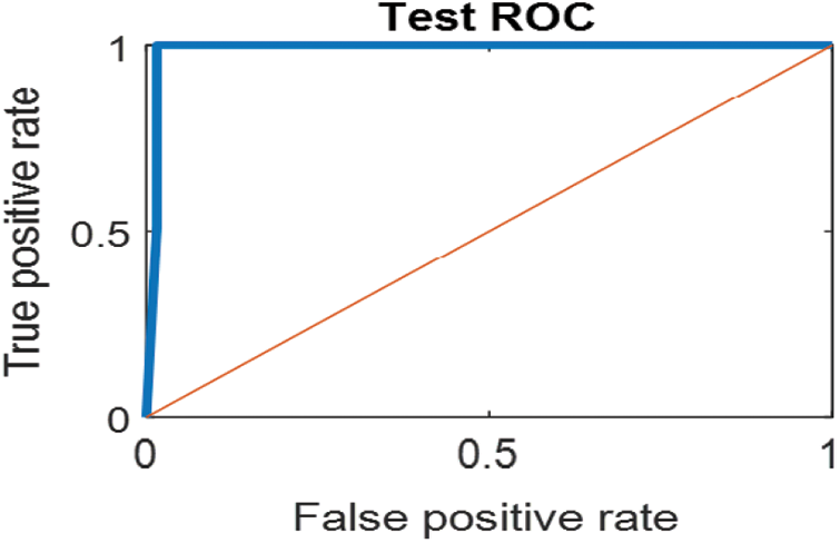
Figure 12: ROC for SVM (1); Normal and abnormal classes
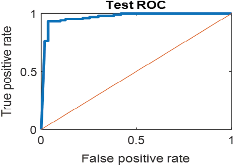
Figure 13: ROC for SVM (2); High and low abnormal classes
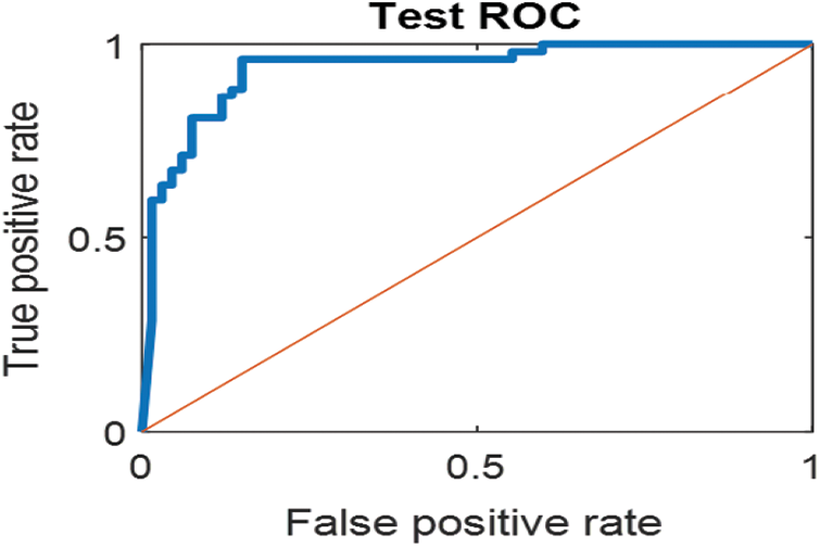
Figure 14: ROC for SVM (3); Carcinoma and sever high-level abnormal classes
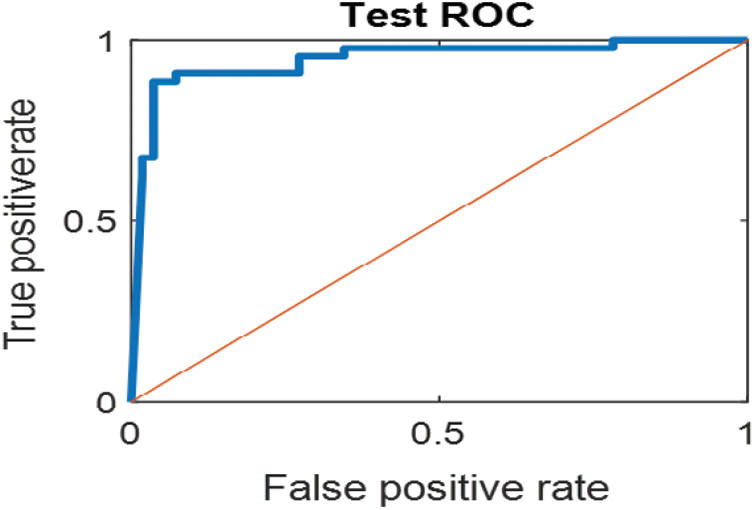
Figure 15: ROC for SVM (4) Mild and moderate low-level abnormal classes
As it is clear in Tab. 2 and Figs. 7 till 11, the recall or sensitivity is high in Model 1 and Model 5. This guarantees that the proposed model can distinguish between normal and abnormal cases to be safe for the patients, besides if they are normal and the type of normalness classes. The lowest sensitivity is in Mild and Moderate from low classes that comes from the high similarities in the images between these two types of biopsies images. That will not be a drawback of the system because these two classes belong to a low level of normalness. Nevertheless, the system obtains high sensitivity in distinguishing between a high level of normalness in the Severe and Carcinoma categories. The precision which indicates the True Negative rate is the highest in normal classes, followed by normal and abnormal results. Precision indicates how accurate the models are out of those predicted positive; in other words, how many of them are positive. The high level of precision in low- and high-level achievement makes this model approximately trustable when intended to be used in medical fields. The area under the curve (AUC) describes the relationship between the True Positive Rate or sensitivity in Y-axes for the receiver of operating characteristics to False positive Rate in the X-axis. The highest area under the curve indicates the perfect distinction between the classes and the lowest False Positive rate. For example, based on Tab. 3, the highest True positive rate is shown by Model 5, while the lowest, which is ∼94%, is shown by Model 3. Overall, all models achieve a high area under the curve. As we mentioned, that makes the system strong in dealing with new biopsies images cases. Since the F1 score is an average of Precision and Recall, it means that the F1 score gives equal weight to Precision and Recall, which is computed for each model separately. All previous studies focused on two classes. Even if the studies are classified as normal and abnormal cases to subclasses, their accuracy was not reached as portrayed by our proposed method. Moreover, some of them suffer from a high computation time, whereas the proposed method in this research is quick and fast. Tab. 4 illustrates the comparison between the presented work with the existed methods in literature.
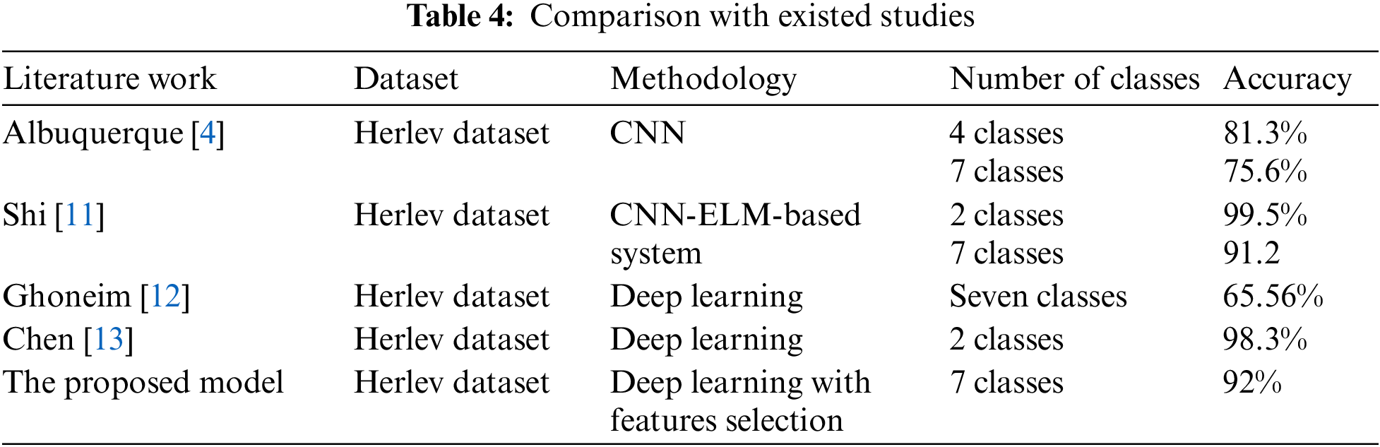
As shown in Table the proposed method achieved the highest accuracy for seven classes when it is compared with literature. The existed work in [14,15] were applied on other dataset based on utilizing preprocessing beside to machine learning algorithms such as SVM, random forest, and fuzzy c mean. Such these methods need computation time, and they are focused on two classes problem.
In this paper, a computer score, automatic Pap smear image analysis system is proposed to analyze cervical cancer in women. The hybrid proposed system using polynomial SVM classifier is proposed to classify the test pap smear cell image into seven classes, namely Superficial, Intermediate, Columnar Normal classes, and Mild, Moderate, Severe Carcinoma in situ for abnormal pap smear images. The features are extracted automatically by predefined existing CNN, which is ResNet101. For obtaining a high level of accuracy, some features are discarded using the feature reduction algorithm PCA. Finally, five cascading SVM models are built to achieve a high level of the confidential system that can be developed to be dependable software in hospitals. The proposed methodology is fast and accurate; the time needs to diagnose one image is less than one second, which is acceptable in medical fields. It is the first system of its type that is able to detect the abnormality then find the degree of abnormality. Also, it overcomes many challenges that were faced by the previous research. The segmentation issue and enhancement of the images besides handcraft features extraction were challenges in traditional computer-aided diagnosis research. This paper proposed a technique for automatically extracting the features without any requirement for the existence of image preprocessing techniques. Skipping this step leads to low computation time, beside to preprocessing may lose some information in the image which leads to reduce the accuracy of the proposed system [43,44]. It also comes with a high level of confidential results to distinguish different classes of pap smear images without consuming time. That is what the clinical field requires. The system can deal with various types of images and conditions regardless of how contrasting the images are and a quick automated for diagnosing the cases besides high accuracy and specificity. The limitations of the system can be overcome by using more datasets, which will cause improvement in the accuracy besides using a high-performance CPU to deal with a huge data.
Acknowledgement: This work was supported by the Ministry of Higher Education Malaysia under the Fundamental Research Grant Scheme (FRGS/1/2021/SKK0/UNIMAP/02/1). The authors would thank the authors of the dataset for making it available online. Also, they would like to thank the anonymous re-viewers for their contribution to enhancing this paper.
Funding Statement: The authors received no specific funding for this study.
Conflicts of Interest: The authors declare that they have no conflicts of interest to report regarding the present study.
1. C. Johnson, in Don’t Wait for Symptoms of Cervical Cancer to Appear, Tech Science Press (Henderson, USA2018. [Online]. Available: https://universityhealthnews.com/daily/cancer/dont-wait-for-symptoms-of-cervical-cancer-to-appear/. [Google Scholar]
2. A. Halim, W. A. Mustafa, W. K. W. Ahmad, H. A. Rahim and H. Sakeran, “Nucleus detection on pap smear images for cervical cancer diagnosis: A review analysis,” Oncologie, vol. 23, no. 1, pp. 73–88, 2021. [Google Scholar]
3. W. A. Mustafa, A. Halim and K. S. A. Rahman, “A narrative review: Classification of pap smear cell image for cervical cancer diagnosis,” Oncologie, vol. 22, no. 2, pp. 53–63, 2020. [Google Scholar]
4. T. Albuquerque, R. Cruz and J. S. Cardoso, “Ordinal losses for classification of cervical cancer risk,” PeerJ Computer Science, vol. 7, pp. 1–21, 2021. [Google Scholar]
5. R. Gibboni, in Meet the Winners of TissueNet: Detect Lesions in Cervical Biopsies, Denver, Colorado, USA: DrivenData Labs, 2020. [Online]. Available: https://www.drivendata.co/blog/tissuenet-cervical-biopsies-winners/. [Google Scholar]
6. T. Li, M. Feng, Y. Wang and K. Xu, “Whole slide images based cervical cancer classification using self-supervised learning and multiple instance learning,” in 2021 IEEE 2nd Int. Conf. on Big Data, Artificial Intelligence and Internet of Things Engineering, ICBAIE 2021, Nanchang, China, ICBAIE, pp. 192–195, 2021. [Google Scholar]
7. R. Mariana Trevisan, T. Alessandra Hermógenes Gomes, S. Raniere, O. Paulo, S. Medeiros et al., “CRIC cervix classification,” Figshare, 2020. [Online]. https://figshare.com/collections/CRIC_Cervix_Cell_Classification/4960286. [Google Scholar]
8. S. N. Atluri and S. Shen, “Global weak forms, weighted residuals, finite elements, boundary elements & local weak forms,” in the Meshless Local Petrov-Galerkin (MLPG) Method, 1st ed., vol. 1. Henderson, NV, USA: Tech Science Press, pp. 15–64, 2004. [Google Scholar]
9. D. N. Diniz, M. T. Rezende, A. G. C. Bianchi, C. M. Carneiro, E. J. S. Luz et al. “A deep learning ensemble method to assist cytopathologists in pap test image classification,” Journal of Imaging, vol. 7, pp. 111, 2021. [Google Scholar]
10. T. N. Kipf and M. Welling, “Semi-supervised classification with graph convolutional networks,” in 5th Int. Conf. on Learning Representations, ICLR 2017 - Conf. Track Proc., Toulon, France, pp. 1–14, 2017. [Google Scholar]
11. J. Shi, R. Wang, Y. Zheng, Z. Jiang, H. Zhang et al., “Cervical cell classification with graph convolutional network,” Computer Methods and Programs in Biomedicine, vol. 198, pp. 105807, 2021. [Google Scholar]
12. Ahmed Ghoneim, Ghulam Muhammad and M. Shamim Hossain, “Cervical cancer classification using convolutional neural networks and extreme learning machines,” Future Generation Computer Systems, vol. 102, pp. 643–649, 2020. [Google Scholar]
13. W. Chen, X. Li, L. Gao and W. Shen, “Improving computer-aided cervical cells classification using transfer learning based snapshot ensemble,” Applied Sciences (Switzerland). vol. 10, no. 20, pp. 1–14, 2020. [Google Scholar]
14. L. Zhang, L. Lu, I. Nogues, R. M. Summers, S. Liu et al., “DeepPap: Deep convolutional networks for cervical cell classification,” IEEE Journal of Biomedical and Health Informatics, vol. 21, no. 6, pp. 1633–1643, 2017. [Google Scholar]
15. W. William, A. Ware, A. H. Basaza-Ejiri and J. Obungoloch, “Cervical cancer classification from pap-smears using an enhanced fuzzy c-means algorithm,” Informatics in Medicine Unlocked, vol. 14, pp. 22–23, 2019. [Google Scholar]
16. A. K. Das, L. B. Mahanta, M. K. Kundu, M. Chowdhury and K. Bora, “Automated classification of pap smear images to detect cervical dysplasia,” Computer Methods and Programs in Biomedicine, vol. 138, pp. 31–47, 2016. [Google Scholar]
17. D. Ravi, C. Wong, F. Deligianni, M. Berthelot, J. Andreu-Perez et al., “Deep learning for health informatics,” IEEE Journal of Biomedical and Health Informatics, vol. 21, no. 1, pp. 4–21, 2017. [Google Scholar]
18. Jiuxiang Gu, Zhenhua Wang, Jason Kuen, Lianyang Ma, Amir Shahroudy, Bing Shuai, Ting Liu,Xingxing Wang, Gang Wang, Jianfei Cai, Tsuhan Chen, “Recent advances in convolustional neural networks,” Pattern Recognition, vol. 77, pp. 354–377, 2018. [Google Scholar]
19. L. Fang, Y. Jin, L. Huang, S. Guo, G. Zhao et al., “Iterative fusion convolutional neural networks for classification of optical coherence tomography images,” Journal of Visual Communication and Image Representation, vol. 59, pp. 327–333, 2019. [Google Scholar]
20. Jürgen Schmidhuber, “Deep learning in neural networks: An overview,” Neural Networks, vol. 61, pp. 85–117, 2015. [Google Scholar]
21. Y. Guo, Y. Liu, A. Oerlemans, S. Lao, S. Wu et al., “Deep learning for visual understanding: A review,” Neurocomputing, vol. 187, pp. 27–48, 2016. [Google Scholar]
22. K. Fukushima and S. Miyake, “Neocognitron: A new algorithm for pattern recognition tolerant of deformations and shifts in position,” Pattern Recognition, vol. 15, no. 6, pp. 455–469, 1982. [Google Scholar]
23. M. Bakator and D. Radosav, “Deep learning and medical diagnosis: A review of literature,” Multimodal Technologies and Interaction, vol. 2, no. 3, pp. 47, 2018. [Google Scholar]
24. S. R. Karanam, Y. Srinivas and M. V. Krishna, “Study on image processing using deep learning techniques,” in Materials Today: Proceedings, Article In Press, pp. 1–6, 2020. https://doi.org/10.1016/j.matpr.2020.09.536. [Google Scholar]
25. K. Zhang, M. Sun, T. X. Han, X. Yuan, L. Guo et al., “Residual networks of residual networks: Multilevel residual networks,” IEEE Transactions on Circuits and Systems for Video Technology, vol. 28, no. 6, pp. 1303–1314, 2018. [Google Scholar]
26. K. He, X. Zhang, S. Ren and J. Sun, “Deep residual learning for image recognition,” in Proc. of the IEEE Computer Society Conf. on Computer Vision and Pattern Recognition, Las Vegas, NV, USA pp. 770–778, 2016. [Google Scholar]
27. J. Deng, W. Dong, R. Socher, L. J. Li, K. Li et al., “ImageNet: A large-scale hierarchical image database,” in 2009 IEEE Conference on Computer Vision and Pattern Recognition, Miami, FL, USA, pp. 248–255, 2009. [Google Scholar]
28. K. He and J. Sun, “Convolutional neural networks at constrained time cost,” in Proc. of the IEEE Computer Society Conf. on Computer Vision and Pattern Recognition, Boston, MA, USA, pp. 5353–5360, 2015. [Google Scholar]
29. T. Zia, “Hierarchical recurrent highway networks,” Pattern Recognition Letters, vol. 119, pp. 71–76, 2019. [Google Scholar]
30. Y. Bengio, P. Simard and P. Frasconi, “Learning long-term dependencies with gradient descent is difficult,” IEEE Transactions on Neural Networks, vol. 5, no. 2, pp. 157–166, 1994. [Google Scholar]
31. X. Glorot and Y. Bengio, “Understanding the difficulty of training deep feedforward neural networks,” Journal of Machine Learning Research, vol. 9, pp. 249–256, 2010. [Google Scholar]
32. Y. Jia, E. Shelhamer, J. Donahue, S. Karayev, J. Long et al., “Caffe: Convolutional architecture for fast feature embedding,” in MM 2014 - Proc. of the 2014 ACM Conf. on Multimedia, Orlando Florida, USA, pp. 675–678, 2014. [Google Scholar]
33. H. Hotelling, “Analysis of a complex of statistical variables into principal components,” Journal of Educational Psychology, vol. 24, no. 6, pp. 417–441, 1933. [Google Scholar]
34. S. P. Mishra, U. Sarkar, S. Taraphder, S. Datta, D. Swain et al., “Multivariate statistical data analysis- principal component analysis (pca),” International Journal of Livestock Research, vol. 7, pp. 60–78, 2017. [Google Scholar]
35. L. C. Paul, A. Al Suman and N. Sultan, “Methodological analysis of principal component analysis (pca) method,” International Journal of Computational Engineering & Management, vol. 16, no. 2, pp. 32–38, 2013. [Google Scholar]
36. L. Smith, “A tutorial on principal components analysis introduction,” Statistics, vol. 51, pp. 1–26, 2002. [Google Scholar]
37. L. Smith, “A tutorial on principal components analysis,” Communications in Statistics-Theory and Methods, vol. 17, no. 9, pp. 3157–3175, 1988. [Google Scholar]
38. R. Geetha, S. Sivasubramanian, M. Kaliappan, S. Vimal and S. Annamalai, “Cervical cancer identification with synthetic minority oversampling technique and pca analysis using random forest classifier,” Journal of Medical Systems, vol. 43, no. 9, pp. 1–19, 2019. [Google Scholar]
39. H. Basak, R. Kundu, S. Chakraborty and N. Das, “Cervical cytology classification using pca and gwo enhanced deep features selection,” SN Computer Science, vol. 2, no. 5, pp. 1–28, 2021. [Google Scholar]
40. S. Adhikary, S. Seth, S. Das, T. K. Naskar, A. Barui and S. P. Maity, “Feature assisted cervical cancer screening through dic cell images,” Biocybernetics and Biomedical Engineering, vol. 41, no. 3, pp. 1162–1181, 2021. [Google Scholar]
41. J. Cao, G. Lv, C. Chang and H. Li, “A feature selection based serial svm ensemble classifier,” IEEE Access, vol. 7, pp. 144516–144523, 2019. [Google Scholar]
42. A. M. Alqudah, H. Alquran, I. Abu-Qasmieh and A. Al-Badarneh, “Employing image processing techniques and artificial intelligence for automated eye diagnosis using digital eye fundus images,” Journal of Biomimetics, Biomaterials and Biomedical Engineering, vol. 39, pp. 40–56, 2018. [Google Scholar]
43. A. M. Alqudah, S. Qazan, H. Alquran, I. A. Qasmieh, and A. Alqudah. “Covid-19 detection from x-ray images using different artificial intelligence hybrid models,” Jordan Journal of Electrical Engineering, vol. 6, no. 2, pp. 168–178, 2020. [Google Scholar]
44. A. M. Alqudah, H. Alquran, and I. A. Qasmieh, “Segmented and non-segmented skin lesions classification using transfer learning and adaptive moment learning rate technique using pretrained convolutional neural network,” Journal of Biomimetics, Biomaterials and Biomedical Engineering, vol. 42, pp. 67–78, 2019. [Google Scholar]
 | This work is licensed under a Creative Commons Attribution 4.0 International License, which permits unrestricted use, distribution, and reproduction in any medium, provided the original work is properly cited. |