DOI:10.32604/cmc.2022.026750
| Computers, Materials & Continua DOI:10.32604/cmc.2022.026750 | |
| Article |
Compiler IR-Based Program Encoding Method for Software Defect Prediction
1School of Information Engineering, Nanjing Audit University, Nanjing, 211815, China
2Department of Computer Science, Kennesaw State University, Kennesaw, 30144-5588, USA
3Information Science and Engineering Department, Hunan First Normal University, Changsha, 410205, China
*Corresponding Author: Chao Xu. Email: xuchao@nau.edu.cn
Received: 04 January 2022; Accepted: 23 February 2022
Abstract: With the continuous expansion of software applications, people's requirements for software quality are increasing. Software defect prediction is an important technology to improve software quality. It often encodes the software into several features and applies the machine learning method to build defect prediction classifiers, which can estimate the software areas is clean or buggy. However, the current encoding methods are mainly based on the traditional manual features or the AST of source code. Traditional manual features are difficult to reflect the deep semantics of programs, and there is a lot of noise information in AST, which affects the expression of semantic features. To overcome the above deficiencies, we combined with the Convolutional Neural Networks (CNN) and proposed a novel compiler Intermediate Representation (IR) based program encoding method for software defect prediction (CIR-CNN). Specifically, our program encoding method is based on the compiler IR, which can eliminate a large amount of noise information in the syntax structure of the source code and facilitate the acquisition of more accurate semantic information. Secondly, with the help of data flow analysis, a Data Dependency Graph (DDG) is constructed on the compiler IR, which helps to capture the deeper semantic information of the program. Finally, we use the widely used CNN model to build a software defect prediction model, which can increase the adaptive ability of the method. To evaluate the performance of the CIR-CNN, we use seven projects from PROMISE datasets to set up comparative experiments. The experiments results show that, in WPDP, with our CIR-CNN method, the prediction accuracy was improved by 12% for the AST-encoded CNN-based model and by 20.9% for the traditional features-based LR model, respectively. And in CPDP, the AST-encoded DBN-based model was improved by 9.1% and the traditional features-based TCA+ model by 19.2%, respectively.
Keywords: Compiler IR; CNN; data dependency graph; defect prediction
With the continuous expansion of software applications, people's requirements for software quality are increasing. People hope to eliminate software defects as much as possible before software release. Nevertheless, the software is larger and complexity, it is difficult to accurately locate the defects of a program at the semantic level. Software defect prediction is a helpful technology for detecting semantic defects. It often encodes the source code into several software features and applies the machine learning method to build defect prediction classifiers, which can estimate the software areas is clean or buggy [1–5]. However, in the modeling process of defect prediction, there are some common challenges: such as how to encode the program, how to extract features from the high dimensionality of defect datasets, how to select the suitable defect training models, and so on. In the paper, we are focused on how to encode the program to extract features for defect prediction.
Software features are the basis of defect prediction. Researchers design various defect features from different dimensions by the analysis of software defect-related factors. Such as the code size, code complexity (e.g., Halstead features based on the number of operators and operands, McCabe features based on dependencies, CK features for object-oriented programs), code churn features, et al. However, those features are traditionally handcrafted with the shallow representation of the programs’ source code or development processing, not for the deep semantic information of the program, which is an important factor for software defect prediction.
To mine the semantic information of the program for building accurate software defect prediction models, some approaches propose to leverage a powerful representation learning algorithm, namely deep learning, to capture the semantic representation of programs, automatically. They often use the Abstract Syntax Trees (AST) of the source code as basis and transform the ASTs’ nodes of the program into tokens vectors. Then the word embedding techniques [6] are applied to encode the tokens vectors as numerical vectors, which are served as inputs to the deep learning models (i.e., Deep Belief Network(DBN) [7], Convolutional Neural Networks(CNN) [8], and Recurrent Neural Networks(RNN) [9], et al.), to automatically extract the semantic features of the program. Programs have well-defined syntax and rich semantics hidden in the ASTs, which can assist to build a more accurate software defect prediction model. However, there are still some deficiencies in capturing program semantics, based on ASTs.
Firstly, Phan et al. [10] shows that the code with the same semantic, such as File1.c and File2.c in Fig. 1, will suffer from varying structures of ASTs, which will affect the performance of defect prediction because of the weight matrices for each node, being determined based on the position in AST.
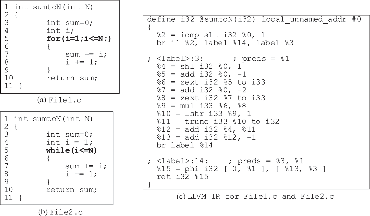
Figure 1: Same semantic with different loop statements example [10]
Secondly, ASTs are not suitable for deep semantic analysis such as data flow analysis, which affects the prominence of software defect features. Figs. 2a and 2b show two code snippets, which were extracted from the commit information of the Redis project in GitHub. The only difference between buggy code and clean code is in line 11 of different flag constants. The AST structure of the two code snippets will be the same, and the only different node is the constant node with a different value, which is ignored by the current ASTs-based method for limiting the number of tokens. Therefore, the current AST-based methods will be failed to capture the defect features in Fig. 2a.
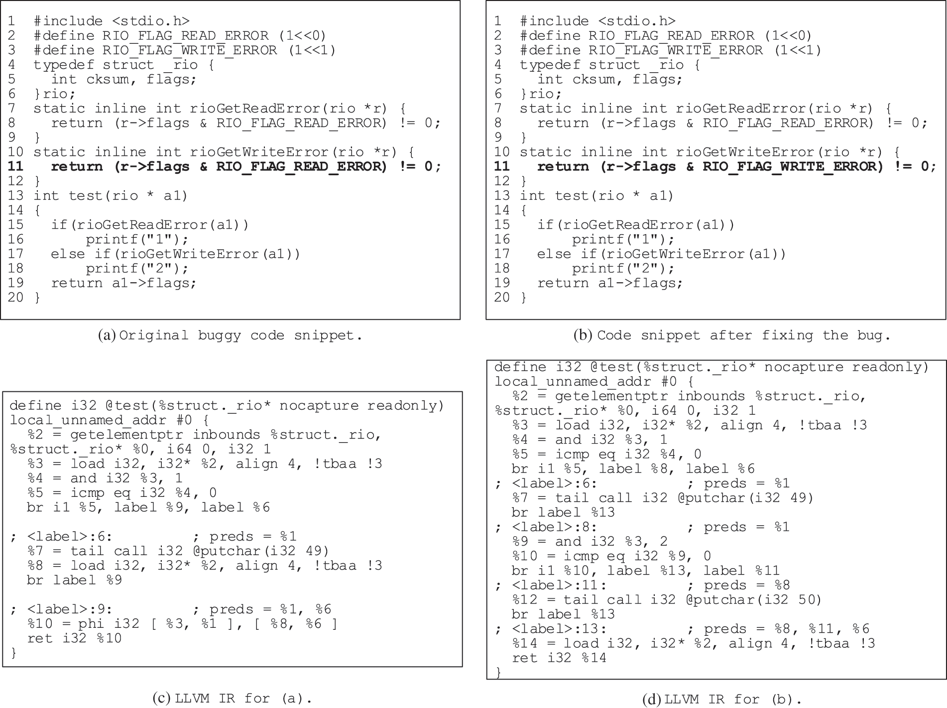
Figure 2: A buggy example from Redis
Furthermore, most of the currently AST-based deep learning defect prediction model seldom considers the type information of variables, which is also an important expression to the semantic of the program. Figs. 3a and 3b show two code snippets. Both define the function of delay10 that takes up ten integers adds time, which is often used in embedded systems to satisfy the precedence constraints. However, Fig. 3a has a defect: because the variable i is used in the function delay10 and has no side-effect, the code of delay10 will be optimized to empty which should break precedence constraints in the calling points. Since the only difference between the two code snippets is the types of i, the ASTs of both will be almost the same. The AST-based defect prediction methods are difficult to capture the defect in Fig. 3a.
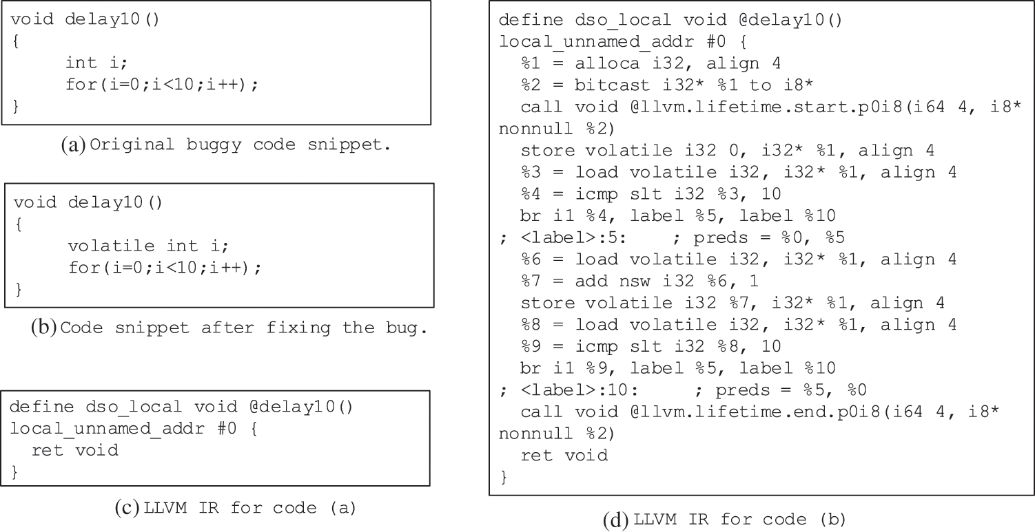
Figure 3: Type-based buggy motivation example
As we all know, the compiler is an essential tool for program transformation, and the AST is also the presentation form of the compiler front end. For better program analysis and optimization, compilers usually design a well-structured internal representation, called Intermediate Representation (IR). Peng et al. [11] shows that the IR is more applicable for learning code representation rather than high-level program language. Motivated by the powerful representation and widely applied in the program analysis, we propose a novel Compiler IR-based program encoding method for defect prediction with CNN model (CIR-CNN) aim to increase the performance in software defect prediction on seven PROMISE datasets. The main contributions of the paper can be summarized as follows:
• Being different from the AST-based program feature extracting methods, this paper encodes the program semantic defect features based on compiler IR, which is expected to obtain more accurate program semantic features for software defect prediction.
• Based on LLVM IR, we designed the token representation, which retains the type information for acquiring the type-related defects features.
• Combined with the data dependency, DDG was built as the basis of program analysis, which is helpful to extract more accurate data dependency features.
• To preserve the semantic and structure information of the graph, we redesigned the weighted adjacency matrix to represent the DDG of the program and used two-dimensional CNN to train and build the defect prediction model.
The outline of this paper is as follows. In the next section, we briefly introduce the related work and background materials used in our work. Section 3 describes our proposed CIR-CNN approach, and the experiments are setup and evaluated in Section 4. Section 5 identifies some limitations of this research work. We conclude the paper and highlights future directions in the last section.
2.1 Software Defect Prediction
Software Defect Prediction (SDP) technology has always been a research hotspot in the field of software engineering, and researchers have carried out extensive research in this field [12–14]. Many machine learning methods have been designed for building defect prediction models [15,16]. Ji et al. [17] proposed an improved Naive Bayes (NB) approach by using kernel density estimation. They compared their methods against four well-known classification algorithms on 34 software releases obtained from 10 open-source projects provided by the PROMISE repository. Li et al. [18] examined C4.5 in defect prediction, which is a kind of Decision Tree (DT) algorithm. Nam et al. [19] proposed TCA+, which adopted a state-of-the-art technique called Transfer Component Analysis (TCA) and the optimized TCA's normalization process to improve cross-project defect prediction. Xia et al. [20] proposed HYDRA, which leverages a genetic algorithm and ensemble learning (EL) to improve cross-project defect prediction. But HYDRA requires massive training data to build and train the prediction models. Tabassum et al. [21] investigated when and to what extent cross-project data are useful for Just-In-Time Software Defect Prediction in a realistic online learning scenario. Zain et al. [22] proposed the 1D-CNN, a deep learning architecture to extract useful knowledge, for identifying and modelling the knowledge in the data sequence, reducing overfitting, and finally, predicting whether the units of code are defects prone. However, these methods are based on traditionally handcrafted features, which are the shallow representation of the programs’ source code or development processing, not for the deep semantic information of the program. They will be affected by people's experience and have weak adaptive ability.
Recently, with the rapid development of deep learning technology and the increasing demand for semantic-based software defect prediction, many researchers explore the application of deep learning methods in software defect prediction. They use deep learning technology to automatically extract the semantic features of programs for building the defect prediction model. Wang et al. [7] leveraged DBN for software defect prediction. They used selected AST sequences taken from source code as input to the DBN model, which generate new expressive features, and used machine learning models for classification. Li et al. [8] proposed a CNN-based defect prediction model, which leveraged word embedding and a CNN model for defect prediction. Their experimental results show that the defect prediction performance of the CNN model is better than Wang's DBN [7]. Pan et al. [23] improved the Li's CNN for within-project defect prediction (WPDP). The experimental results show that their CNN model was comparable to Li's CNN model, and outperformed the state-of-the-art machine learning models significantly. Hoa et al. [9] leveraged tree-based LSTM models to predict defects. However, their results were not as good as the results of Li's CNN model [8]. Sun et al. [24] proposed an unsupervised domain adaptation based on the discriminative subspace learning (DSL) approach for CPDP. However, these methods are based on the AST of source code, which may be affected by the implementations of program. At the same time, they are not suitable for deep semantic analysis and insensitive to type related defects, which shown in Figs. 1–3
There was also research on deep defect prediction targeting assembly code [10], which leveraged a CNN model to learn from assembly instructions. However, the assembler is architecture related, and it is difficult to transplant to other platforms.
Intermediate Representation (IR) is the foundation for a compiler to realize cross-language analysis and optimization. Based on the IR, the compiler analyzes the semantics of the source code and executes a variety of optimization passes to eliminates the useless code of the source program, which usually contains noisy semantic information. Therefore, the normalized and meaningful semantic information is preserved in the final IR by compiler optimization, and we can get the outstanding semantic features by IR. Different compilers have their own IRs, and in this paper, we use the IR of the LLVM compiler called LLVM IR for the following reasons.
• Unlike the IR of GCC, which has multiple IR such as GENERIC, GIMPLE, RTL, and so on, the IR of LLVM is unique. It is well defined and more suitable for processing and transforming.
• The LLVM IR representation aims to be lightweight and low-level while being expressive, typed, and extensible at the same time. It is convenient to extract type information for helping defect prediction.
• There are many program conversion and analysis tools for LLVM IR, such as JLang, RetDec, etc. We can transform different high-level programming source code and even binary code to LLVM IR easily.
From the perspective of LLVM IR, the semantic information of the program is more prominent. For example, in Fig. 1, although File1.c and File2.c have different loop structures, their LLVM IRs are the same, shown in Fig. 1c.
And in Fig. 2, the rioGetWriteError and rioGetReadError are inline functions. The buggy code shown in Fig. 2a defines the two methods the same. The condition code in line 15 and 17 will be considered the same, and lines 17 and 18 will be removed safely during the optimization of the compiler. Therefore, the final LLVM IRs of buggy code and clean code are differently shown in Figs. 2c and 2d. For the two code snippets in Figs. 3a and 3b, the LLVM IRs are shown in Figs. 3c and 3d, respectively. From these two IR snippets, the differences are outstanding. For the code in Fig. 3a, all of the codes are optimized and deleted, and the function becomes empty (see as Fig. 3c). We can easily distinguish the semantic features from these IR differences.
At the same time, compiler IR is easy for control flow analysis and data flow analysis to represent the relationship between instructions and data, which is helpful for the semantic features extracting. Therefore, we suspect that if the deep-learning-based feature extraction method was applied to the compiler IR, we could get more exactly the programs’ semantic features. It should be noted that, although ASTs are also one former of compiler IR, the compiler IR mentioned in this paper is the IR that after compilation optimization and directly used as the input of the code generation of the compiler.
A CFG is a directed graph, G = (V, E) where V is the set of vertices {v1, v2, …, vn} and E is the set of directed edges {<vi, vj>, <vk, vl>, …}. In the CFG, each vertex represents a basic block that is a linear sequence of IRs with one entry point (the first IR executed) and one exit point (the last IR executed). And the directed edges show the control flow paths. CFG can display the relationship between basic blocks, dynamic execution status, and statement table corresponding to each basic block in a process. However, it cannot deal with well the relationship between instructions in basic blocks. For example, in Fig. 4, Fig. 4b is the LLVM IR for Fig. 4a. We can see that the CFG has only one node because there is no branch in the source code. If we analyze the semantics of the source code based on this CFG, we can form the order dependency shown in Fig. 4c. These will lead to the segmentation of the most critical defect features between the instruction 2 and instruction 7. Therefore, we will further be able to construct the DDG based on the CFG.
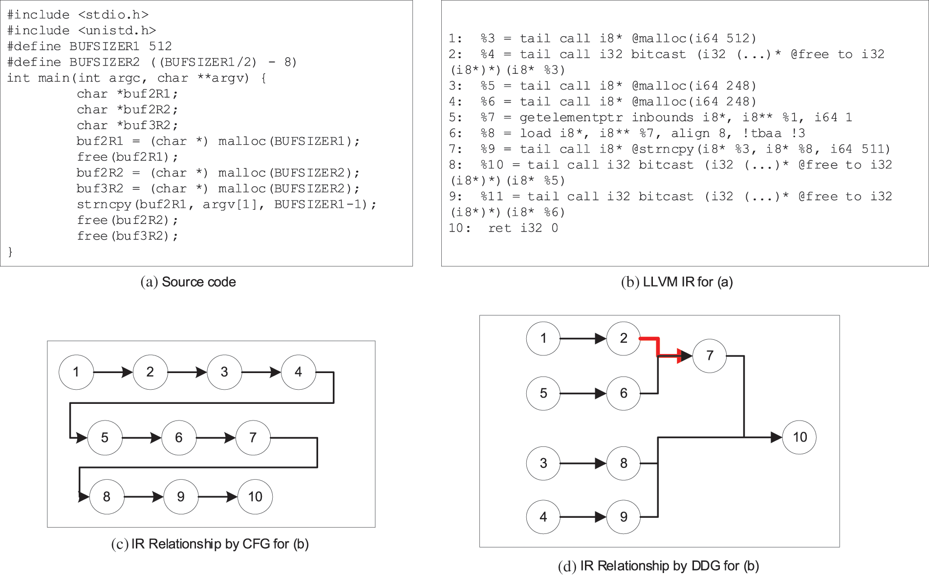
Figure 4: The motivation example for DDG
A DDG is also a directed graph, G = (V, E) where V is the set of vertices {v1, v2, …, vn} and E is the set of directed edges {<vi, vj>, <vk, vl>, …}. However, in the DDG, each vertex represents an IR, and the directed edges show the data dependencies. We use the IRi represents the ith IR in the program. If IRi must execute before IRj, there is one directed edge from IRi to IRj. For example, the DDG of Fig. 4b is Fig. 4d. Instruction 7 and instruction 2 are adjacent to use the same storage space “%3”, and instruction 2 is a function call that may have the side effect. Therefore, instruction 2 must execute before instruction 7, and the directed edge from instruction 2 to instruction 7 is added, which will make the defect features more prominent.
Convolutional Neural Networks (CNN) is a feedforward neural network with a structure to convolution calculation [25]. It has been successfully applied in many practical fields, including image classification, speech recognition, and natural language processing [26–35].
CNN includes a feature extractor composed of convolution layers and pooling layers. A convolution layer of CNN usually contains several feature maps. Each feature map is composed of some rectangular neurons. Neurons in the same feature plane are only connected with some adjacent neurons and share weights. These shared weights are convolution kernels. The convolution kernel is generally initialized in the form of a random decimal matrix. In the process of network training, the convolution kernel will learn to obtain reasonable weights. The direct benefit of convolution kernel is to reduce the connection between network layers and reduce the risk of overfitting. The pooling layer follows the convolution layer and is also composed of multiple feature maps. Each feature map of the pooling layer uniquely corresponds to one feature surface of the upper layer, and the max-pooling is often used.
In recent years, some researchers [7–9] have explored the effect of CNN in building software defect prediction models and reached positive conclusions. However, at present, software defect prediction mainly focuses on one-dimensional CNN, the scene where CNN performs better is two-dimensional CNN, such as image recognition. Therefore, in our work, we leverage two-dimensional CNN which is trained by the adjacency matrix of the program for effective feature generation from LLVM IR.
Fig. 5 shows the steps of our compiler IR-based program embedding method for defect prediction over CNN: a) Transform the Program to Compiler IR; b) Generate DDG from IR; c) Extracting and Encoding tokens for the DDG Nodes; d) Program encoded by the weighted adjacency matrix. e) Then, the weighted adjacency matrix will be used as inputs to train and build the CNN model for software defect prediction. f) When a program needs to predict defects, we first obtain the weighted adjacency matrix of the program and then input it into the built model, which will give the prediction results of clean or buggy.
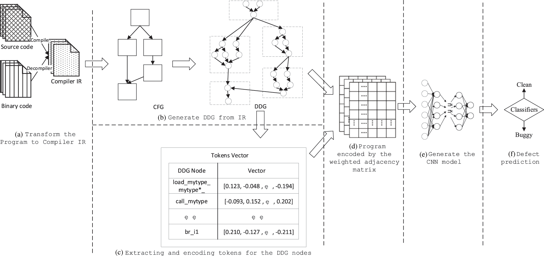
Figure 5: The framework of the CIR-CNN
3.2 Transform the Program to Compiler IR
The compiler IR is a kind of normalized representation of the program, which preserves the semantics of the program. The first step of our method is to transform the program to the LLVM IR. Specifically, the transformation to LLVM IR can be categorized into two cases.
• Input is the source code. We will use the corresponding compilers to complete the transform. For example, we can use Clang to transform the C and C++ source code to LLVM IR and use the JLang to transform the Java source code to LLVM IR.
• Input is the binary code. We will use the RetDec tool to decompile it to LLVM IR.
In order to obtain more accurate program semantic information to assist software defect prediction, we first extract the CFG from IR, then construct the DDG of the program by CFG.
Fig. 6 shows an example of transforming a piece of IRs (Fig. 6a) to CFG (Fig. 6b) and then generating DDG (Fig. 6c). In Fig. 6a, the first line is the definition of the function with the following IRs included.
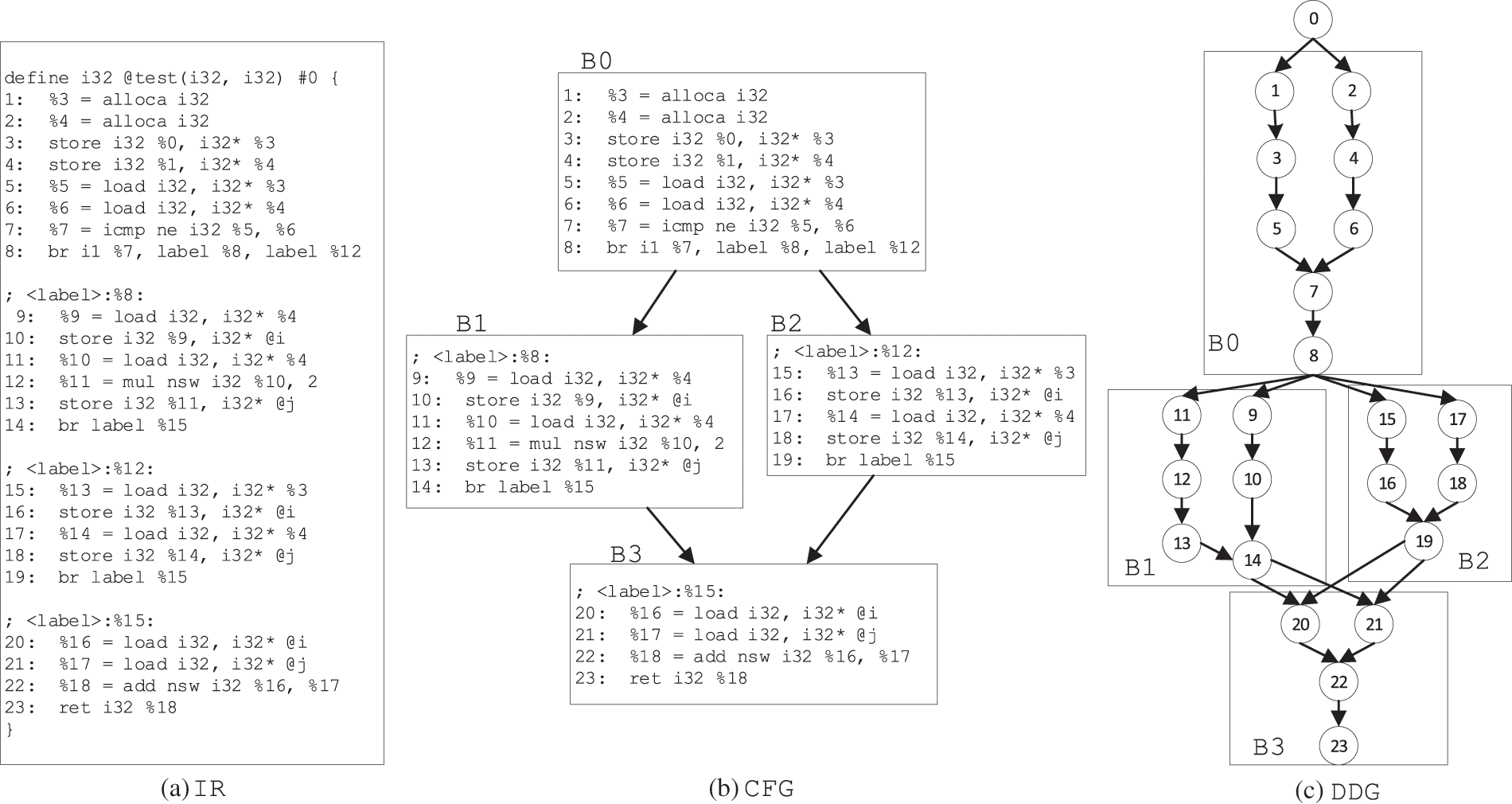
Figure 6: The example of IR to DDG transformation
For the CFG construction, the primary work is to analyze the branch IRs. In Fig. 6a, the first seven IRs are the load/storage and comparison instructions, and they are sequences executed without branch. Until the eighth “br” instruction, the program will jump to different positions according to the comparison result of “%7”. Therefore, the first eight statements are in the same basic block and can be organized as a node in CFG, called B0 in Fig. 6b. Similarly, IRs in lines 9–14, 15–19 and 20–23 are also basic blocks, which are corresponding to the nodes B1, B2 and B3 in Fig. 6b, respectively. Then, we analyze the last IR of each node in CFG and extract the control flow information to form the edges of CFG. For example, in the last IR of B0, we can see that the execution after B0 is the IR at “label 8” or “label 12”. And “label 8” corresponds to the entry of the B1 node, and “label 12” corresponds to the entry of the B2 node. Hence, the converted CFG has an edge from B0 to B1 and an edge from B0 to B2. Similarly, we can also get the edges from B1 to B3 and B2 to B3, and form the CFG shown in Fig. 6b.
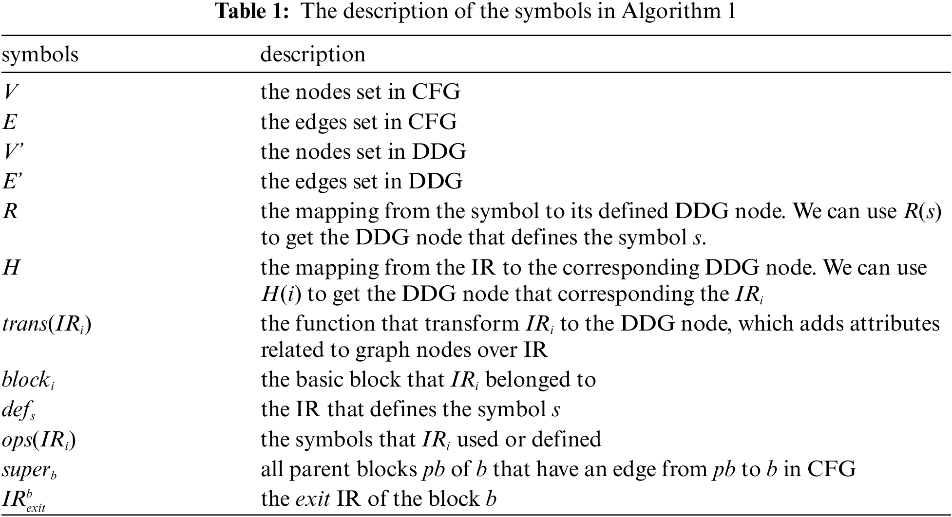
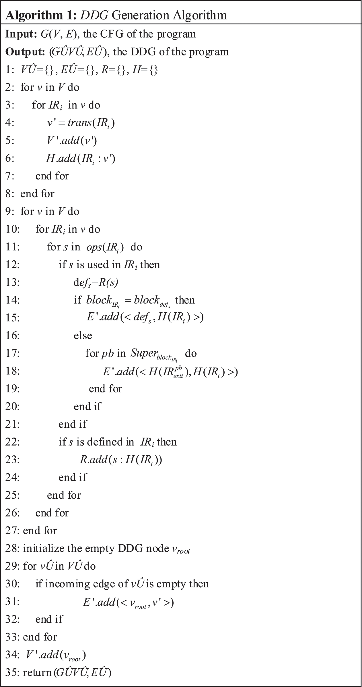
When we get the CFG of the program, DDG can be generated by Algorithm 1, where we give the symbol definition in Tab. 1.
In the algorithm, for each node in CFG, each IR is traversed in turn, encapsulated as a DDG node by trans function. And the relationship between IR and DDG node is saved in H (lines 2–8). Then we traverse every node of CFG again, and analyze the attribute of each symbols s that of IRi defined or used. If the attribute of s is defining, we will establish the mapping between s and H(IRi) and save it in R (lines 22–24). For example, for the first IR in Fig. 6, the operand “%3” indicates that a 32-bit space is defined, and the mapping relationship from “%3” to H(IR1) will be established and saved to R. If the symbol s is used in the IRi, we will search the defs in R. If s and defs are in the same basic block (line 14), an edge from H(defs) to H(IRi) will be added to
3.4 Extracting and Encoding Tokens for the DDG Nodes
To make the CNN-based deep learning technology automatically extract software features from DDG for defect prediction, we encode each node of DDG into numerical vectors. Similar to the existing mainstream methods, the encoding process includes two stages: a) Extracting the tokens from the nodes; b) Transforming the tokens into numerical vectors.
For the first step, the nodes of DDG are encapsulated by the compiler IR that is commonly divided into operator and operands, so we designed the tokens of DDG nodes also containing two parts: operator string and operands string. For the operator string, if it is the “call” instruction, we will set the token string by the specific calling method. When the calling method is a system library method such as “printf”, the calling method name will be used as the operator string token. Otherwise, the string “call” will be used as the operator string token. For example, the operator string of “%3 = call i8* @malloc(i64 512)” is “malloc”, and the operator string of “%3 = tail call i8* @calScore(i64 512)” is “call”, where “calScore” is a user-defined method. For the operator that is not the “call”, the string of operator name in LLVM IR is used as its operator string token. For example, the operator string of “store i32%0, i32* %3” is “store”. The operands string is represented by the type of operands in IR, which has the following three situations.
• If the type of the operand is the basic system type in LLVM, such as “int32”, “int8”, et al., we will use the corresponding string in LLVM to represent them, such as “i32”, “i8”, et al.;
• If the type of the operand is defined by ourselves, we will use “mytype” to represent it.
• If the type is a pointer type, we will leave “*” after the type.
After getting the operator string and operands string, we use “_” to connect them as the token of the DDG node. For example, the token of node “storei32%0, i32 ∗ %3” is “store_i32_i32∗”, and the token of node “%3 = call i8* @malloc(i64 512)” is “malloc_i8∗”.
When the DDG nodes are converted into tokens, a method similar to Wang's DBN [7] is applied. We first build a mapping between integers and tokens, and each token is associated with a unique integer identifier which ranges from 1 to the total number of tokens. Then, the word embedding technique is used to further map each DDG token into a numerical vector, which is trained regarding the context of each token. However, being different from one-dimensional word embedding in NLP [6], we extract the association information of tokens based on graph structure. Although we can obtain one-dimensional tokens through graph traversal, it will destroy the graph structure, affecting the word embedding and in turn defect prediction. In order to maintain the information on the graph structure, we design a graph-based word embedding method based on CBOW [6]. We select the parent node and child nodes of the central DDG node as the context for training the distributed representation of the DDG node to preserve the graph structure to the greatest extent. For example, to evaluate the node 7 in Fig. 6, we will use its parents of nodes 5 and 6, and its child of node 8 as its context. Eq. (1) describes our way to capture context for the central word n and calculate the projection value (P is the parent of the word n and C is all the children of the word n). After the CBOW based graph word embedding transformation, tokens appearing in similar context tend to have similar vector representations that are close in the feature space, which can benefit CNN in learning the program semantics in certain contexts.
3.5 Program Encoded by Weighted Adjacency Matrix
At present, the most successful application of CNN is mainly in the field of image recognition, of which the input is two-dimensional. We thought that if the DDG is transformed into two-dimensional expression, it will be conducive to CNN model to obtain better classification effect. Since the adjacency matrix is the widely used two-dimensional graph representation, we also use it for our purposes. When DDG nodes are transformed into tokens and encoded into numerical vectors, the program can be expressed as a weighted adjacency matrix M by N × N, where N is the number of tokens. In order to meet the constraints of CNN model on the fixed input shape, we arrange the nodes in DDG in descending order of occurrence frequency, and then take the first N nodes as the observation nodes construct the adjacency matrix. We use mij to represent the weight in the row i and column j of the adjacency matrix M, which can be calculated by Eq. (2). In Eq. (2), nij denotes the number of edges from tokeni to tokenj in DDG, tixdenotes the ith value in the numerical vector of tokeni, k is the length of the numerical vector, and ε is an infinitesimal number to prevent the denominator from being zero.
The weight calculation is critical to the prediction model. The basic principle of software defect prediction is to detect whether the program has the defects characteristics in the semantic level. In our method, we have normalized the semantics of the program into the DDG. The weight should reflect the characteristics of the DDG. Since DDG is a graph, its characteristics can be measured by the structural information of the graph, which can be expressed by node and edges. So we calculate the weight from two dimensions. The first is for the nodes. The more similar the two nodes are, the greater the value will be. Here, we calculate the Euclidean distance between nodes and find the reciprocal, which is the denominator of Eq. (2). The second is the dependency strength between nodes, which is expressed by the number of edges, i.e., the molecular of Eq. (2).
In this step, we take advantage of CNN's powerful capability of feature generation, and capture semantic and local structural information of the weighted adjacency matrix represented program. Because we focus on the impact of IR-based encoding method on the defect prediction, and engage CNN only as an application, we adopt a similar architecture and parameters of Li's CNN [8]. In particular, our CIR-CNN consists of one two-dimensional convolutional layers and max-pooling layers to extract global patterns, a flattening layer, one dense layer, and finally, a logistic regression classifier to predict whether a LLVM IR file was buggy. Our CIR-CNN framework is built with Keras tools, using TensorFlow as the backend. We take minibatch Stochastic Gradient Descent (SGD) as an optimization strategy and use the Adam algorithm as the optimizer to adjust the learning rate. The detail information of our CNN model is shown in Tab. 2. Here, because the two-dimensional CNN is used in our method, the kernel size of the convolution layer and the pool size of the pooling layer cannot be obtained from Li's CNN [8]. Therefore, we determine their values through experiments. See the Section 4 for details.

Logistic Regression as the final classifier. We process each file in both training set and test set following the above steps, and obtain the weighted adjacency matrix of each source file. After we train our model using the training files with their corresponding labels, both the weights and the biases in our CNN and Logistic Regression are fixed. Then for each file in the test set, we feed it into our defect prediction model and the final classifier will give us a value, indicating the probability of this file being buggy.
4 Experimental Setup and Analysis
In this section, we compare our proposed method with the performance of existing methods. In particular, our experiments were based on the following questions:
•RQ1: How to set the hyperparameters in two-dimensional CNN?
•RQ2: Does our proposed CIR-CNN method improve the performance of within-project defect prediction (WPDP)?
•RQ3: Does our proposed CIR-CNN method improve the performance of cross-project defect prediction (CPDP)?
All of our experiments were run on a Linux server with one Intel(R) Xeon(R) Gold 5218 CPU and one GeForce RTX 2080 Ti GPU.
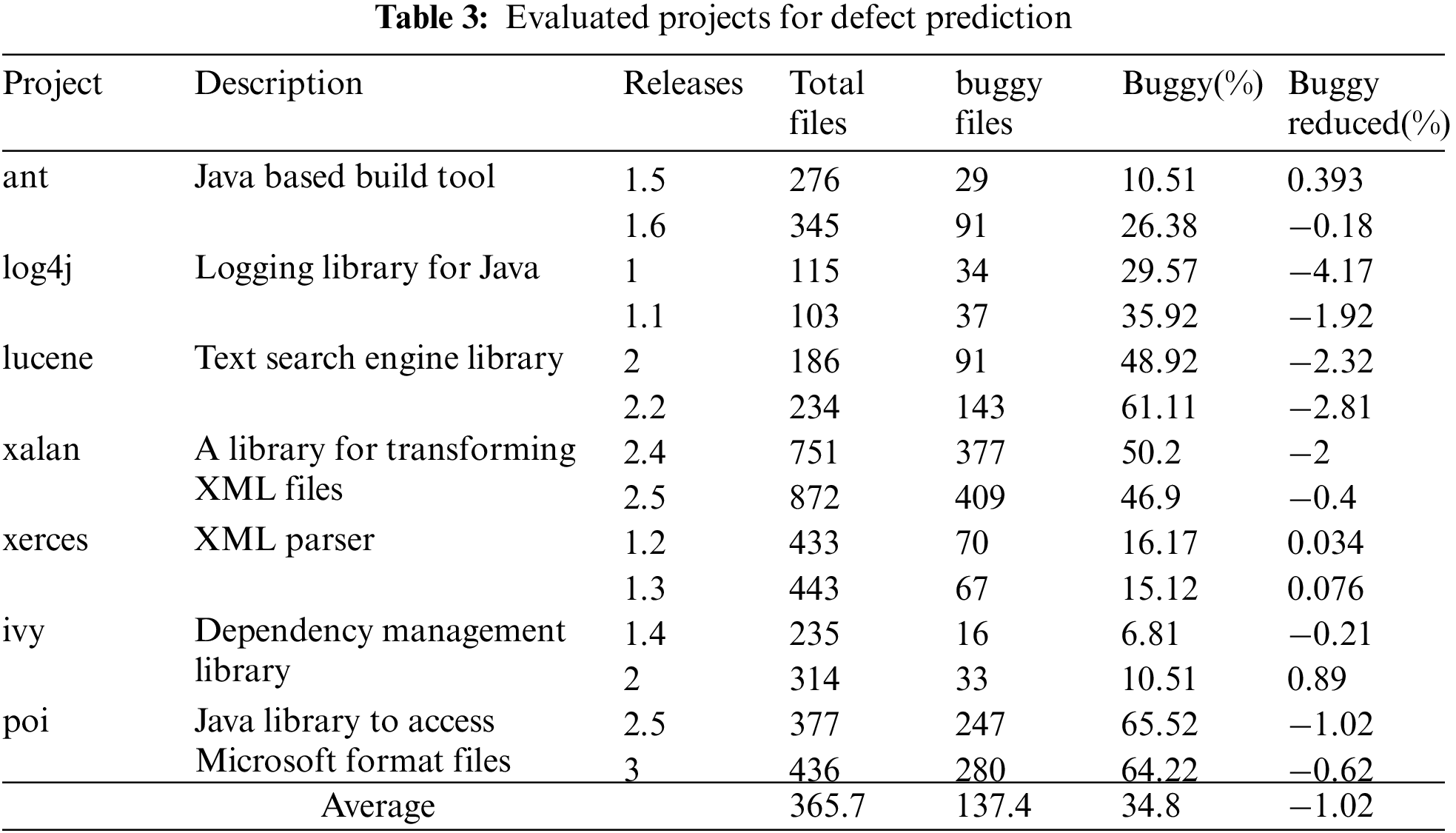
To facilitate the replication and verification of our experiments, we collected Java projects from the PROMISE data repository, where the version numbers, the class name of each file, and most importantly, the defect labels for each source file are provided. In total, 7 Java projects are collected, and we select two versions of each project as our dataset. Tab. 3 shows the details of these projects, including project description, versions, the total number of files, the buggy number of files, the buggy rate, and the buggy rate reduce percentage caused by file delete of our data preprocessing.
Since our CIR-CNN method based on the LLVM IR, we downloaded the corresponding versions of the projects from open source repositories rather than using the existing traditional features. To parse source files into LLVM IR, we utilized a tool called JLang. It enables translating Java 7 source code into LLVM IR, except for some advanced reflection features, primarily related to generic types. Hence, due to the limited functionality of JLang, several Java source files could not be parsed correctly, which may have hampered data preprocessing. We adopted the following four strategies to solve the problem.
• Correct the source file grammar so that JLang could parse, such as replace the variable symbol “enum” with “enum1”.
• Delete part of the source code that could not parse.
• Delete the file directly and add the corresponding classes files to JLang's dependency library.
• Delete the project if most of the files in the project fail to parse.
To measure the performance of the defect prediction, we computed the F1 score which is composed of Precision and Recall and widely used for evaluating the performance of software defect prediction [7,8]. We estimated the values of Precision, Recall, and F1 score based on four statistics: True Positives (TP), False Positives (FP), False Negatives (FN), True Negatives (TN). Their definitions are as follows: if a file is classified as defective when it is truly defective, the classification is TP. If the file is classified as defective when it is clean, then the classification is FP. If the file is classified as clean when it is defective, then the classification is FN. Finally, if the issue is classified as clean but in fact is clean, then the classification is TN. We use the above statistics to estimate Precision, Recall, and F1 score by Eqs. (3)–(5), respectively.
Both Precision and Recall reflect the effectiveness of our prediction model. According to the above formulas, Precision is the ratio between the number of true positives over the number of link candidates that are predicted as true links by our model. On the other hand, Recall is the percentage of the number of true positives over the total amount of true links. Importantly, between Precision and Recall, there is usually an inverse relationship where higher Precision might come with lower Recall and vice versa. Thus, the F1 score, which is the harmonic mean of Precision and Recall, is used to synthesize the two metrics into a summary measure.
To evaluate the performance of our proposed CIR-CNN method, we conducted a comparative experiment from two aspects: WPDP and CPDP.
In WPDP, we compare CIR-CNN with the Traditional LR, DBN, and CNN. The Traditional LR is a Logistic Regression classifier. It is based on 20 traditional code features [36] to build a logistic regression model for defect prediction. These features have been widely used in previous work to build effective defect prediction models [19]. The DBN is a state-of-the-art method that leverages a deep belief network (DBN) to automatically learn semantic features using token vectors extracted from the programs’ ASTs. For the defect prediction performance of the traditional LR and DBN, we directly cite the experimental results in [7]. The CNN method is a variant of DP-CNN that directly feeds the CNN-learned features to the final classifier without combining traditional features. It is also based on the ASTs but utilizes CNN for automated feature generation from source code. We implement the CNN method by Keras with the same network architecture and parameter settings as Li's CNN [8].
In the aspect of CPDP, we take DBN-CP and TCA+ [19] as our comparisons baseline methods which are also evaluated in Wang's paper [7]. And the same as WPDP, we use the performance results from the Wang's paper [7] for easy comparison.
4.4 Performance of CIR-CNN under Different Hyperparameters (RQ1)
As a two-dimensional CNN model, its hyperparameters of kernel size and pool size will also be two-dimensional, for which the parameters in Li's CNN [8] cannot be used. Therefore, we use lunce, poi, xalan and xerces from PROMISE as the dataset by WPDP evaluation to tune the hyperparameters. The WPDP evaluation method is shown in the next section. The kernel size and pool size are varied within the range of {2 × 2, 3 × 3, 4 × 4, 5 × 5}, and the remaining parameters are set according to Tab. 2. Fig. 7 shows the performance and average performance of the four projects in WPDP under different kernel size and pool size. Where, the x-axis is the value of two super parameters, and the y-axis is the F1 score and average F1 score of each project under the hyperparameters setting corresponding to x-axis.
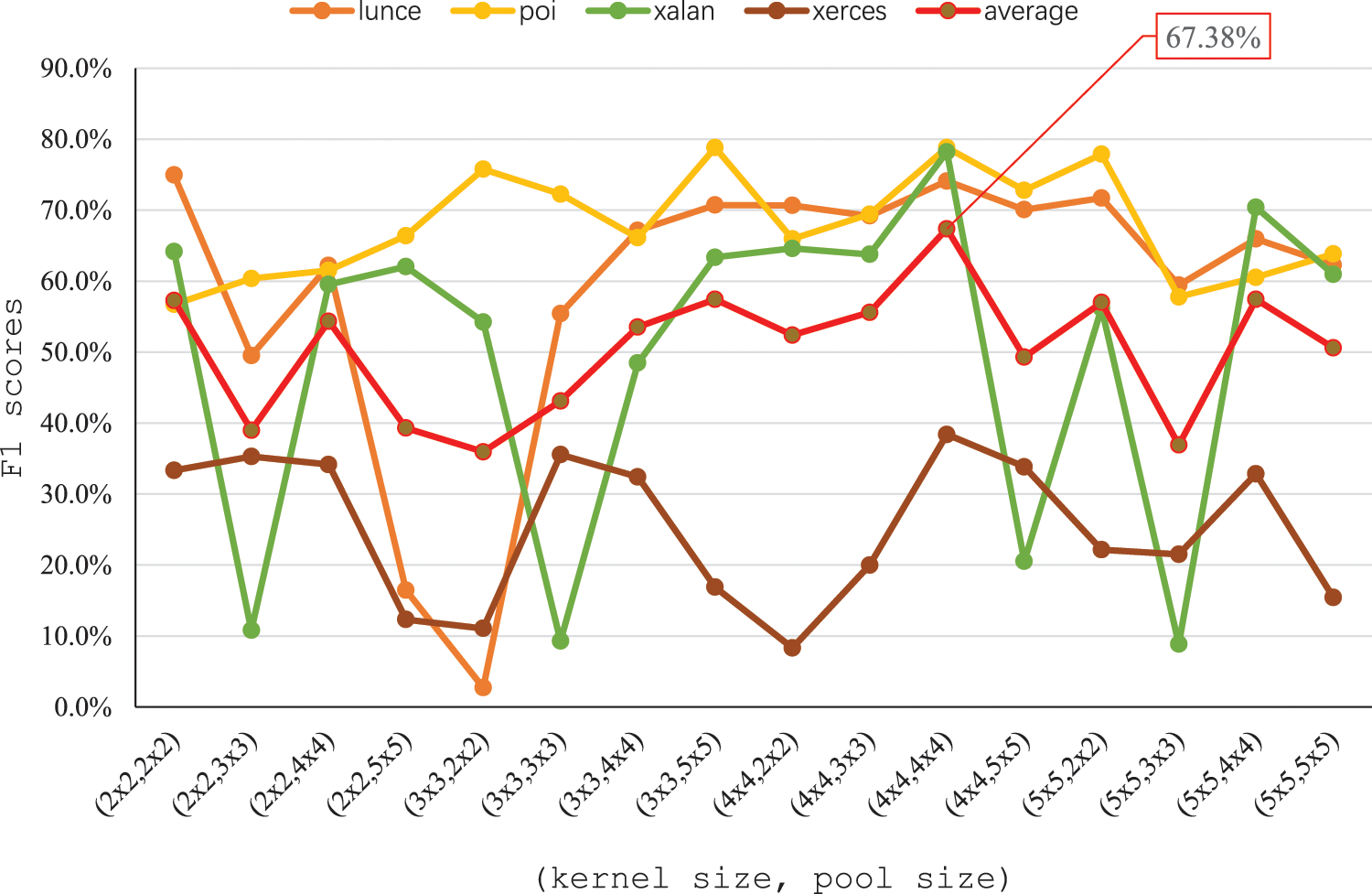
Figure 7: The performance of different hyperparameters
From the Fig. 7, we can see that different hyperparameters settings have different effects on the prediction performance of different projects. For example, for xalan and xerces, their F1 scores fluctuate greatly by the hyperparameters, while for lunce and poi, their F1 scores fluctuate less. These may be due to different defect characteristics. Therefore, in order to maximize the performance of software defect prediction, we use the point with the largest mean value as the selected value for the two hyperparameters, that is, the kernel size and pool size are set to 4 × 4.
4.5 Performance of CIR-CNN in WPDP (RQ2)
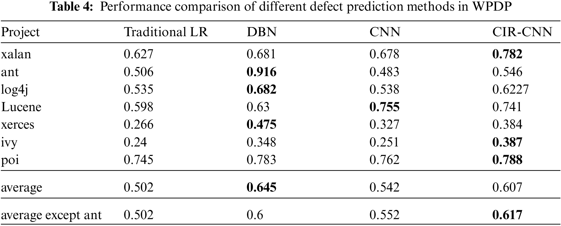
To evaluate the performance of CIR-CNN in WPDP, we carried out comparative experiments on the seven projects listed in Tab. 3. We use the older version to train prediction models and the newer version as the test set to evaluate the trained models. The F1 score on each project by applying the four competing methods is shown in Tab. 4. The highest F1 score of them is shown in bold. For example, in the xalan project, we use xalan 2.4 as the training set and xalan 2.5 as the test set, and we get the F1 score of defect prediction is 0.627, 0.681, 0.678, and 0.782 for Traditional LR, DBN, CNN, and CIR-CNN, respectively. And the best result is 0.782 for CIR-CNN. From the experimental results, we can see that the CIR-CNN method is better than the Traditional LR method in all cases. On average, the F1 score of CIR-CNN is 0.105 higher than the traditional LR method, which improves 20.9%. These indicate that the features obtained by compiler IR have a better prospect than traditional features in defect prediction. By comparing the F1 score of CIR-CNN with DBN and CNN, we can find that for most cases, the F1 score of CIR-CNN is competitive with these of DBN. Although DBN is 0.038 higher than CIR-CNN on average, it is mainly contributed by the ant project. If the ant project is excluded, the F1 score of CIR-CNN is 0.017 higher than DBN on average. More significantly, CNN whose network structure and parameters are the same as CIR-CNN, gets a lower F1 score than CIR-CNN for most cases. On average, the F1 score of CIR-CNN is 0.065 higher than CNN, which improves 12%. These show that the compiler IR-based feature can get better performance than AST-based features in WPDP.
4.6 Performance of CIR-CNN in CPDP (RQ3)
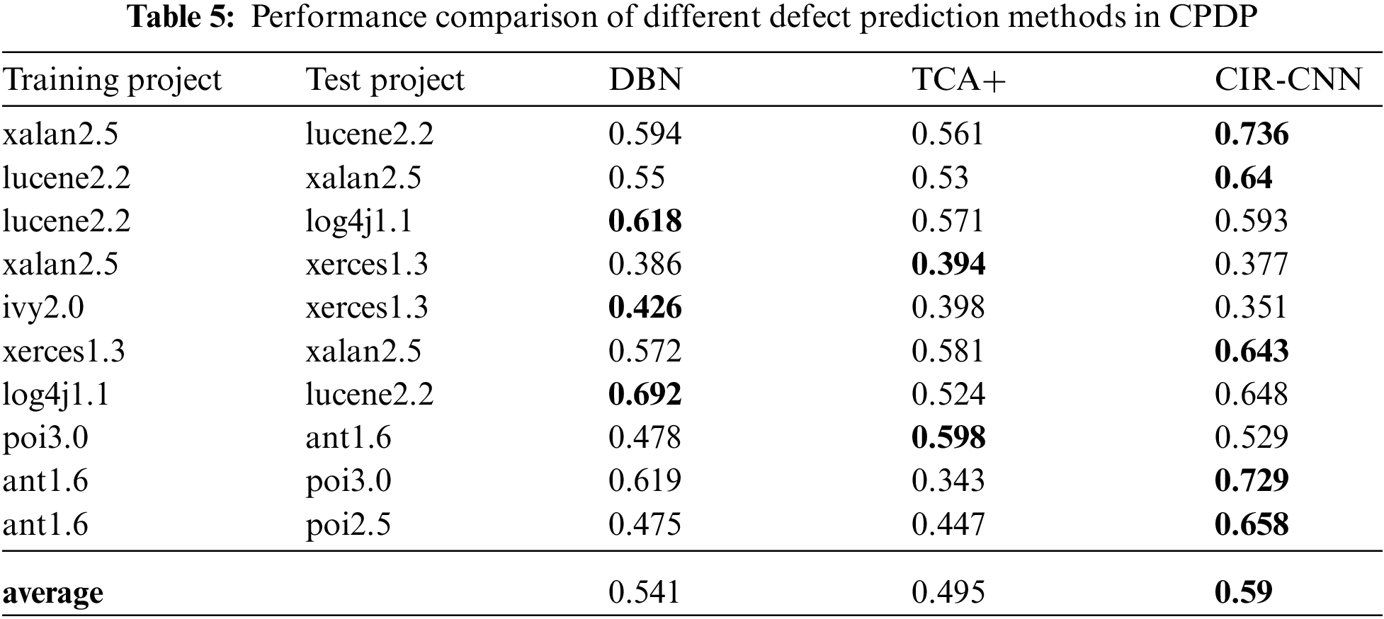
To evaluate the performance of CIR-CNN in CPDP, we collect a set of 10 cross-project test pairs. Each experiment takes two versions separately from two different projects, the one used as the training set and the other used as the test set. The F1 score on each pair projects by applying the three competing methods is shown in Tab. 5. The highest F1 score of them is shown in bold. From the experimental results, we can see that the CIR-CNN is still competitive in CPDP. For half of the cases, CIR-CNN can get the highest F1 score. On average, the F1 score of CIR-CNN is 0.095 higher than TCA+ and 0.049 higher than DBN, which is 19.2% and 9.1% improvements respectively. These indicate that compiler IR-based features are a better choice for CPDP.
From the above experimental results, we can see that our method can get better performance than above references methods in many projects, and we think the main reasons are as follows. Firstly, the LR and TCA+ are based on the traditional features. These features are designed by the people's experience, and may not be able to adapt to different programming modes [7,8]. Li's CNN and Wang's DBN are based on the AST of the source program. Due to the same semantics may implement with different grammatical structure, the extracted features are not obvious, as described in Section 1. However, our method is based on the compiler IR. It eliminates the syntax differences at the source program, which can obtain more accurate semantic features, shown in Section 2.2. And furthermore, we combined with the type information to extract more type-related features. Therefore, our method can use more and accurate information to train the defect prediction model and get better performance.
For the comparative analysis, we compare our CIR-CNN method with CNN, which is the state-of-the-art within project defect prediction technique. Since the original implementation of CNN is not released, we have reimplemented our version of CNN by Keras. Although we strictly followed the procedures described in their work, our new implementation may not reflect all the implementation details of the original CNN. However, we test our implemented one with the data provided by their work. The results show that our version can achieve very similar results to the original one. Hence, we are confident that our implementation reflects the performance of the original CNN.
We conducted our experiments using seven open-source projects in the PROMISE dataset, and they might not be representative of all software projects. Besides, we only evaluated CIR-CNN on projects written in Java language. Given projects that are not included in the seven projects or written in other programming languages (e.g., C++ or Python), our proposed method might generate better or worse results. To make CIR-CNN more generalizable, in the future, we will conduct experiments on a variety of projects including open-source and closed-source projects, and extend our method to other programming languages.
When we convert the dataset source program to compiler IR, we delete a few source files due to JLang's limited syntax support of the Java programming language. However, from the statistical results, the deleted files did not make the buggy rate of the dataset change significantly. On average, the buggy rate only increased by 1.02% as compared with the original PROMISE repository. Therefore, we claim that deletion of files would not influence the validity of our results that much.
To improve the ability of software defect prediction at the semantic level, we propose a novel compiler IR-based program encoding method for defect prediction with the CNN model (CIR-CNN). Specifically, we first transform the source code and binary code into the compiler IR by compiler and decompiler tools, respectively. Then, the data dependency graph (DDG) is constructed over CFG by data flow analysis. Next, we encode the DDG to the weighted adjacency matrix by word embedding technology combined. Finally, we use the weighted adjacency matrix as the input and the existing mature CNN network structure to train and build the defect prediction model.
Based on the compiler IR, our method eliminates the noise information at the syntax level of the source program and obtains more essential program semantic information for software defect prediction. Therefore, the extracted defect features will be more accurate. At the same time, through the token representation with types, the detection ability of type-related defects is improved. Therefore, our method can achieve good results in both WPDP and CPDP. We examined the performance of features automatically extracted by the compiler IR-based program encoding method on two file-level defect prediction tasks, i.e., within-project defect prediction (WPDP) and cross-project defect prediction (CPDP). In WPDP, our experiments on seven open-source projects show that averagely, CIR-CNN improves the AST-based CNN and traditional feature-based methods by 20.9% and 12%, respectively, in terms of F1 score in defect prediction. And CIR-CNN is competitive with the state-of-the-art DBN-based method. In CPDP, our experiments on ten pairs of open source projects show that averagely, CIR-CNN improves the AST-based DBN and traditional features-based TCA+ methods by 19.2% and 9.1%, respectively.
The novelty of this paper is that we combined with the two-dimensional CNN and proposed a compiler IR based program encoding method for software defect prediction, which can get the performance increase in seven projects of PROMISE dataset.
As the future works, we are planning to make our method more generalizable and effective. Specifically, we will conduct experiments on more projects and more deep learning models, combine CIR-based features with other features, extend our method to both other programming languages and binary code, and also integrate different programming languages for coordinated prediction.
Funding Statement: This work was supported by the Universities Natural Science Research Project of Jiangsu Province under Grant 20KJB520026 and 20KJA520002; the Foundation for Young Teachers of Nanjing Auditing University under Grant 19QNPY018; the National Nature Science Foundation of China under Grant 71972102 and 61902189.
Conflicts of Interest: The authors declare that they have no conflicts of interest to report regarding the present study.
1. S. Feng, J. Keung, J. Liu, Y. Xiao, X. Yu et al., “ROCT: Radius-based class overlap cleaning technique to alleviate the class overlap problem in software defect prediction,” in IEEE 45th Annual Computers, Software, and Applications Conf. (COMPSAC), Madrid, Spain, pp. 228–237, 2021. [Google Scholar]
2. L. Qiao, G. Li, D. Yu and H. Liu, “Deep feature learning to quantitative prediction of software defects,” in IEEE 45th Annual Computers, Software, and Applications Conf. (COMPSAC), Madrid, Spain, pp. 1401–1402, 2021. [Google Scholar]
3. X. Liu, H. Li and X. Xie, “Intelligent radar software defect prediction approach and its application,” in IEEE 20th Int. Conf. on Software Quality, Reliability and Security Companion (QRS-C), Macau, China, pp. 32–37, 2020. [Google Scholar]
4. S. Albahli and G. Nabi, “Defect prediction using akaike and Bayesian information criterion,” Computer Systems Science and Engineering, vol. 41, no. 3, pp. 1117–1127, 2022. [Google Scholar]
5. F. Matloob, M. G. Taher, T. Nasser, A. Shabib, A. Munir et al., “Software defect prediction using ensemble learning: A systematic literature review,” IEEE Access, vol. 9, pp. 98754–98771, 2021. [Google Scholar]
6. T. Mikolov, I. Sutskever, K. Chen, G. S. Corrado and J. Dean, “Distributed representations of words and phrases and their compositionality,” NIPS, Lake Tahoe Nevada, USA, vol. 2, pp. 3111–3119, 2013. [Google Scholar]
7. S. Wang, T. Liu, J. Nam and L. Tan, “Deep semantic feature learning for software defect prediction,” IEEE Transactions on Software Engineering, vol. 46, no. 12, pp. 1267–1293, 2020. [Google Scholar]
8. J. Li, P. He, J. Zhu and M. R. Lyu, “Software defect prediction via convolutional neural network,” in IEEE Int. Conf. on Software Quality, Reliability and Security(QRS-C), Prague, Czech Republic, pp. 318–328, 2017. [Google Scholar]
9. K. D. Hoa, P. Trang, W. N. Shien, T. Truyen, G. John et al., “A deep tree-based model for software defect prediction,” arXiv: Software engineering, 2018. [Online]. Available: https://arxiv.org/abs/1802.00921. [Google Scholar]
10. A. V. Phan, M. L. Nguyen and L. T. Bui, “Convolutional neural networks over control flow graphs for software defect prediction,” in IEEE 29th Int. Conf. on Tools with Artificial Intelligence (ICTAI), Boston, MA, USA, pp. 45–52, 2017. [Google Scholar]
11. D. L. Peng, S. X. Zheng, Y. T. Li, G. L. Ke, D. He et al., “How could neural networks understand programs?,” arXiv: Programming languages, 2021. [Online]. Available: https://arxiv.org/abs/2105.04297. [Google Scholar]
12. B. S. Alqadi and J. I. Maletic, “Slice-based cognitive complexity metrics for defect prediction,” in IEEE 27th Int. Conf. on Software Analysis, Evolution and Reengineering (SANER), London, ON, Canada, pp. 411–422, 2020. [Google Scholar]
13. A. A. Bangash, H. Sahar, A. Hindle and K. Ali, “On the time-based conclusion stability of cross-project defect prediction models,” Empirical Software Engineering, vol. 25, no. 6, pp. 1–38, 2020. [Google Scholar]
14. V. Rohit and A. M. R. Syed, “Estimation of target defect prediction coverage in heterogeneous cross software projects,” International Journal of Information System Modeling and Design (IJISMD), vol. 12, no. 1, pp. 73–93, 2021. [Google Scholar]
15. B. Mumtaz, S. Kanwal, S. Alamri and F. Khan, “Feature selection using artificial immune network: An approach for software defect prediction,” Intelligent Automation & Soft Computing, vol. 29, no. 3, pp. 669–684, 2021. [Google Scholar]
16. M. S. Daoud, S. Aftab, M. Ahmad, M. A. Khan, A. Iqbal et al., “Machine learning empowered software defect prediction system,” Intelligent Automation & Soft Computing, vol. 31, no. 2, pp. 1287–1300, 2022. [Google Scholar]
17. H. Ji, S. Huang, X. Lv and Y. Wu, “Empirical studies of a kernel density estimation based naive Bayes method for software defect prediction,” IEICE Transactions on Information and Systems, vol. 102, no. 1, pp. 75–84, 2019. [Google Scholar]
18. B. Li, B. Shen, J. Wang, Y. Chen, T. Zhang et al., “A Scenario-based approach to predicting software defects using compressed C4.5 model,” in IEEE 38th Annual Computer Software and Applications Conf., Vasteras, Sweden, pp. 406–415, 2014. [Google Scholar]
19. J. Nam, S. J. Pan and S. Kim, “Transfer defect learning,” in ICSE, San Francisco, USA, pp. 382–391, 2013. [Google Scholar]
20. X. Xia, D. Lo, S. J. Pan, N. Nagappan and X. Wang, “HYDRA: Massively compositional model for cross-project defect prediction,” IEEE Transantions on Software Engineering, vol. 42, no. 10, pp. 977–998, 2016. [Google Scholar]
21. S. Tabassum, L. L. Minku, D. Feng, G. G. Cabral and L. Song, “An investigation of cross-project learning in online just-in-time software defect prediction,” in ICSE, Seoul, Korea, pp. 554–565, 2020. [Google Scholar]
22. Z. M. Zain, S. Sakri, N. Halimatul and R. M. Parizi, “Software defect prediction harnessing on multi 1-dimensional convolutional neural network structure,” Computers, Materials & Continua, vol. 71, no. 1, pp. 1521–1546, 2022. [Google Scholar]
23. C. Pan, M. Lu, B. Xu and H. Gao, “An improved CNN model for within project software defect prediction,” Applied Sciences, vol. 9, no. 10, pp. 21–38, 2019. [Google Scholar]
24. Y. Sun, Y. Sun, J. Qi, F. Wu, X. Jing et al., “Unsupervised domain adaptation based on discriminative subspace learning for cross-project defect prediction,” Computers, Materials & Continua, vol. 68, no. 3, pp. 3373–3389, 2021. [Google Scholar]
25. J. Sulam, A. Aberdam, A. Beck and M. Elad, “On multi-layer basis pursuit, efficient algorithms and convolutional neural networks,” IEEE Transactions on Pattern Analysis and Machine Intelligence, vol. 42, no. 8, pp. 1968–1980, 2020. [Google Scholar]
26. K. Sathya and M. Rajalakshmi, “RDA-CNN: Enhanced super resolution method for rice plant disease classification,” Computer Systems Science and Engineering, vol. 42, no. 1, pp. 33–47, 2022. [Google Scholar]
27. A. H. Ossama, A. R. Mohamed, H. Jiang, L. Deng, G. Penn et al. “Convolutional neural networks for speech recognition,” IEEE/ACM Transactions on Audio, Speech and Language Processing (TASLP), vol. 22, no. 10, pp. 1533–1545, 2014. [Google Scholar]
28. Z. Wang, X. Wang and G. Wang, “Learning fine-grained features via a CNN tree for large-scale classification,” Neurocomputing, vol. 275, no. 1, pp. 1231–1240, 2018. [Google Scholar]
29. X. R. Zhang, X. Sun, X. M. Sun, W. Sun and S. K. Jha, “Robust reversible audio watermarking scheme for telemedicine and privacy protection,” Computers, Materials & Continua, vol. 71, no. 2, pp. 3035–3050, 2022. [Google Scholar]
30. X. R. Zhang, W. F. Zhang, W. Sun, X. M. Sun and S. K. Jha, “A robust 3-D medical watermarking based on wavelet transform for data protection,” Computer Systems Science & Engineering, vol. 41, no. 3, pp. 1043–1056, 2022. [Google Scholar]
31. L. Chen, B. Wang, W. Yu and X. Fan, “Cnn-based fast hevc quantization parameter mode decision,” Journal of New Media, vol. 1, no. 3, pp. 115–126, 2019. [Google Scholar]
32. R. Zhang, F. Zhu, J. Liu and G. Liu, “Depth-wise separable convolutions and multi-level pooling for an efficient spatial CNN-based steg analysis,” IEEE Transactions on Information Forensics and Security, vol. 15, no.1, pp. 1138–1150, 2020. [Google Scholar]
33. S. Khurana, G. Sharma, N. Miglani, A. Singh, A. Alharbi et al., “An intelligent fine-tuned forecasting technique for covid-19 prediction using neuralprophet model,” Computers, Materials & Continua, vol. 71, no.1, pp. 629–649, 2022. [Google Scholar]
34. N. K. Trivedi, V. Gautam, A. Anand, H. M. Aljahdali, S. G. Villar et al., “Early detection and classification of tomato leaf disease using high-performance deep neural network,” Sensors, vol. 21, no no. 23, pp. 7987, 2021. [Google Scholar]
35. P. Kaur, S. Harnal, R. Tiwari, F. S. Alharithi, A. H. Almulihi et al., “A hybrid convolutional neural network model for diagnosis of COVID-19 using chest X-ray images,” Int. J. Environ. Res. Public Health, vol. 18, no. 22, pp. 12191, 2021. [Google Scholar]
36. Z. He, F. Peters, T. Menzies and Y. Yang, “Learning from opensource projects: An empirical study on defect prediction,” in ESEM, Baltimore, MD, USA, pp. 45–54, 2013. [Google Scholar]
 | This work is licensed under a Creative Commons Attribution 4.0 International License, which permits unrestricted use, distribution, and reproduction in any medium, provided the original work is properly cited. |