Computers, Materials & Continua DOI:10.32604/cmc.2022.026943
Article

Printed Surface Defect Detection Model Based on Positive Samples

Xin Zihao1, Wang Hongyuan1,*, Qi Pengyu1, Du Weidong2, Zhang Ji1 and Chen Fuhua3

1School of Computer Science and Artificial Intelligence, Changzhou University, Changzhou, Jiangsu, 213164, China
2Focusight Technology Co, Changzhou University, Changzhou, Jiangsu, 213164, China
3West Liberty University, 208 University Drive, West Liberty, 26074, USA
*Corresponding Author: Wang Hongyuan. Email: hywang@cczu.edu.cn
Received: 07 January 2022; Accepted: 14 March 2022

Abstract: For a long time, the detection and extraction of printed surface defects has been a hot issue in the print industry. Nowadays, defect detection of a large number of products still relies on traditional image processing algorithms such as scale invariant feature transform (SIFT) and oriented fast and rotated brief (ORB), and researchers need to design algorithms for specific products. At present, a large number of defect detection algorithms based on object detection have been applied but need lots of labeling samples with defects. Besides, there are many kinds of defects in printed surface, so it is difficult to enumerate all defects. Most defect detection based on unsupervised learning of positive samples use generative adversarial networks (GAN) and variational auto-encoders (VAE) algorithms, but these methods are not effective for complex printed surface. Aiming at these problems, In this paper, an unsupervised defect detection and extraction algorithm for printed surface based on positive samples in the complex printed surface is proposed innovatively. We propose a kind of defect detection and extraction network based on image matching network. This network is divided into the full convolution network of feature points extraction, and the graph attention network using self attention and cross attention. Though the key points extraction network, we can get robustness key points in the complex printed images, and the graph network can solve the problem of the deviation because of different camera positions and the influence of defect in the different production lines. Just one positive sample image is needed as the benchmark to detect the defects. The algorithm in this paper has been proved in “The First ZhengTu Cup on Campus Machine Vision AI Competition” and got excellent results in the finals. We are working with the company to apply it in production.

Keywords: Unsupervised learning; printed surface; defect extraction; full convolution network; graph attention network; positive sample

1  Introduction

Defect detection of printed surface refers to judging whether the printed surface has defects, and defect extraction refers to defining the type of defects and extract the shape. With the improvement of printing technology, the background of product packaging printing is becoming more and more complex. So the defect detection of printed surface can no longer be carried out manually now. Nowadays there are two main methods of defect detection in industry: traditional image processing and deep learning. Although the traditional image processing is fast, but all images need to be shot at the same angle and position, which requires more precision for production line and needs manual assistance in some times. For different printed surface, the algorithms of traditional image processing need to be redesigned, which prolongs the cycle of product development. Another method is the objection detection based on deep learning, such as YOLO(You Only Look Once) [1], Cascade R-CNN(Region-Based Convolutional Neural Network) [2] etc. Despite this kind of methods can detect the defects of products with strong robustness, it needs a lot of industrial data to screen and label data.

Different from the common surfaces such as steel and concrete, the surface of prints is complex and has many types of defects. For example, the cigarette packages have reflective material printing and some factories use complex printing process such as ‘gold stamping’. There are many types of defects, such as dirty spots, ink lines, ghosting, white leakage and so on. Moreover, the shapes of these defects have great randomness, so it is difficult to enumerate all defect types by labeling data sets and use supervised defect detection algorithms. At present, most methods of defect detection are using supervised learning algorithms based on both positive and negative samples. There were few studies on unsupervised algorithms just based on positive samples. These studies used GAN(Generative Adversarial Network) [3,4] and VAE(Variational Auto-Encoder) [5,6] to train by learning many positive samples to predict the style of the images to be detected in the case of positive images and detect defects. However, the method based on GAN and VAE can only used for the images with smooth surface, simple background and few types of defects such as steel, so it means methods above can not work well in defect detection of printed surface.

In view of the above, defect detection and extraction of printed surface based on the complex background of positive samples has become a hot topic in the field of computer vision. In this paper, the matching algorithm of key points based on full convolutional neural network is applied to defect detection of printed surface in the complex background based on positive samples proposed innovatively, and the graph attention network is creatively used to correct the position deviation different product inspection lines due to the misplacement of cameras and products.

We propose an unsupervised defect extraction algorithm based on positive samples in complex background without manual data annotation innovatively. There is no need for a large number of positive samples, and just need one positive sample image as a benchmark. And using full convolution neural network to extra the key points of printed images for matching, compared with the traditional algorithm, it has higher matching accuracy, and the speed is faster than the SIFT, which is commonly used in images matching. To improve the robustness of the network for different kinds of matter, we using graph attention network instead of the traditional brute force matching algorithm.

2  Related Works

2.1 Defect Detection Algorithms

In the field of defect detection, the unsupervised algorithms based on positive samples are mostly based on images with simple defect types such as steel and concrete, or repetitive background texture images such as textiles. Mei et al. [7] proposed a network based on image pyramid and convolution denoising auto encoder(CDAE) to get different resolution channels. Reconstruction residuals of the training patches are used as the indicator for direct pixelwise defect prediction, and the reconstruction residual map generated in each channel is combined to generate the final inspection result. However, this method is only suitable for the images with repetitive texture background, and can not be applied to the other surface detect detection. Tao et al. [8] used Cascaded auto-encoder(CASAE) to reconstruct images, segment and located defects on metal surfaces and they use cascading network which can generate a pixel-wise prediction mask based on semantic segmentation. We found through the experiments that the CDAE and CASAE is invalid for the defect extraction problem of printed matter surface based on complex background of positive samples.

2.2 Image Matching Algorithms

The meaning of image matching is to match two or more images by improving the saliency and invariance of feature descriptors. Compared with the defect detection algorithms were commonly used, the defect detection algorithms based on image matching only needs a small number of positive samples, and do not need to manually label the data set, but also can extract defects with strong randomness effectively. It is very suitable for surface defect extraction of printed surface with complex background.

Traditional image matching algorithms include SIFT [9], ORB [10], speeded up robust features (SURF) [11], A-SIFT [12] and so on. Fast corner detector [13] is the first system that applies matching learning algorithm to high-speed corner detection and carries out scale-invariant feature transformation.

With the development of deep learning, a large number of image matching algorithms based on deep learning have emerged, such as universal correspondence network (UCN) [14], learned invariant feature transform (LIFT) [15], LF-Net(Learning local features from images) [16], SuperPoint [17] and so on. Universal correspondence network matches by retaining the feature space of geometric or semantic similar. LF-Net generates a scale-space score map along with dense orientation estimates to select the key points. Image patches around the chosen key points are cropped with a differentiable sampler(STN) and fed to the descriptor network, which generates a descriptor for each patch. The full convolution model of SuperPoint can directly input the full-scale images and output pixel-level key point positions and feature descriptors in a single forward pass. With the rapid development of image processing [18,19], compared with the traditional algorithms, algorithms based on deep learning are more flexible.

In addition, there are a large number of studies on whether the matching of feature points is correct and extracting deeper information to get robust descriptor [20–22]. The traditional random sample consensus(RANSAC) [23,24] algorithm can use geometric information to alleviate the problem that it is difficult to distinguish whether the matching is correct due to the complete dependence on descriptor. GMS [25] algorithm leads to the principle that there are more matching points in the neighborhood of the matched feature points through the smoothness of the motion and count the number of matching points in the neighborhood to judge whether a match is correct or not. Deep learning usually focus on using convolutional neural network(CNN) to learn better sparse detectors and local descriptors from images in the field of image matching. SuperGlue [26] uses graph network to match two sets of local features by jointly finding correspondences and rejecting non-matchable points.

By integrating the previous work, we innovatively proposed feature points extraction network based on full convolution neural network and using graph attention mechanism to match the images, which can deal with the problem of defect detection in complex background better. The idea of defect extraction used in this paper to work out the key point vector and feature descriptor vector of positive samples and samples to be detected respectively through the feature points extraction network, and then match them through the graph attention network. Finally, correcting the images and then making residual, the area that have differences are regarded as defects. The overall framework is shown in Fig. 1.

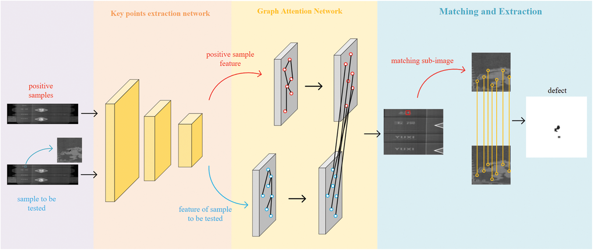
Figure 1: Defect extraction algorithm. We propose a kind of defect extraction based on image matching network which divided into the full convolution network of feature points extraction and the graph attention network. This model can input the full-scale images directly and extract the defects in a single forward pass

3  Key Points Extraction Network

The feature points extraction network designed in this paper is shown in Fig. 2. Because the images taken by industrial defect detection equipment are generally high-definition images, we design a full convolution neural network which can input full-scale images. The network can complete a forward propagation in a short time, and obtain the pixel level key point scoring matrix and descriptor vector of key points. The key point extracting network can be subdivided into feature coding network, key point generation network and feature descriptor generation network.

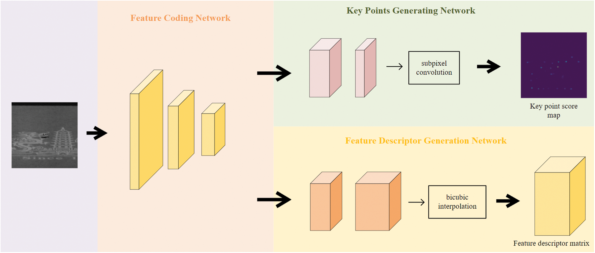
Figure 2: Feature point extraction network. The feature coding network is a full convolution neural network which can input full-scale images, and the output of feature coding network is the input of key points generating network and feature descriptor generation network

3.1 Feature Coding Network

The feature coding network designed in this paper is similar to VGG(Visual Geometry Group) network [27], which is composed of convolution layer, spatial down sampling and nonlinear activation function. The main function of the feature coding network is to compress the spatial dimension of the input full-scale image. The feature coding network has eight 3×3 convolution layers sized 64-64-64-64-128-128-128-256 which both performance and speed can be balanced. There are three maximum pooling layers in the network, which can reduce the length and width of the original images to one eighth and convolution layers can increase the number of channels. It is used to learn the key point generation network and feature descriptor generation network. The size of the input image is I∈RH×W, and the size of output tensor is I′∈RH8×W8×128.

3.2 Key Points Generation Network

The key points generation network input is the output of the feature coding network, which can be regarded as the decoding network of the feature coding network. In the key points generation network, the input of I′∈RH8×W8 through two-dimensional convolution and output IG′∈RH8×W8×65. The responses across the 65 values in the channel dimension should sum to 1 so we add an extra value to represent no key point in the image just like we always add the “background” class in the object detection. When there is no key point in the 8×8 patch, the value of the 64th first bins should ideally be 0 and the 65th should equals to 1 and then remove the 65th bin. Finally, through sub-pixel convolution [28] which shown in Fig. 3, the final key points evaluation map Ip∈RW×H is obtained. Each value of the evaluation map represents the score of the key points of the corresponding pixels in the original image, and the appropriate key points are selected through the threshold t.

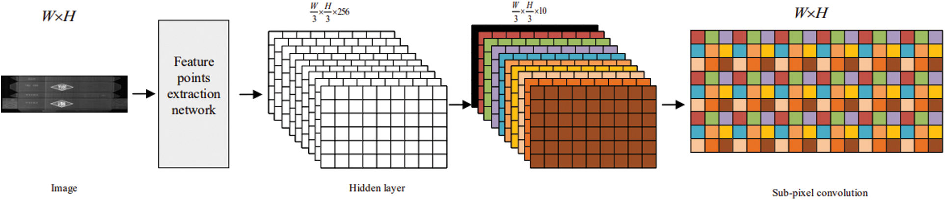
Figure 3: Sub-pixel Convolution. A sub-pixel convolution layer aggregates the feature map from low-resolution space and recovers the size of input image in a single step. The 8×8 patch is too large to show, so we use 3×3 patch here to explain the sub-pixel convolution

3.3 Feature Descriptor Generation Network

As same as above, the feature descriptor generation network is the output of the key points generation network. After two-dimensional convolution, the compressed feature descriptor is obtained, which size of the input image is I′∈RH8×W8×128 and the size of output tensor is ID′∈RH8×W8×256, Because of the feature descriptors of adjacent pixels are similar, the bicubic interpolation algorithm [29] is used to expand the feature descriptors to ID∈RH×W×256. The feature of each pixel in the original image ID∈RH×W×256 corresponds to an unique vector αi∈R256 in the feature descriptors.

4  Graph Attention Network

The descriptor vector of the key points of the image can not directly process by the conventional convolutional neural network. So we use the attention mechanism of graph network to carry out image matching and defect extraction. After the feature points are extracted, the self attention and the cross attention mechanism belong to graph network are adopted, in which the self attention mechanism is applied to an image alone, in order to select the key points with good robustness for matching. The cross attention mechanism acts on two images simultaneously, and the two images exchange descriptor vectors for iterations to find similar key points in the two images. After several iterations of self attention cross attention graph network, the two images output more robust descriptor vector. Through the inner product operation of descriptor vector, the matching score matrix can be obtained. After thresholding the score matrix, the matching of the two images is completed. To get the defects, we must make adjustment for gray scale residuals for both images, and the differences are defects. Fig. 4 shows a flowchart of image matching of a graph attention network.

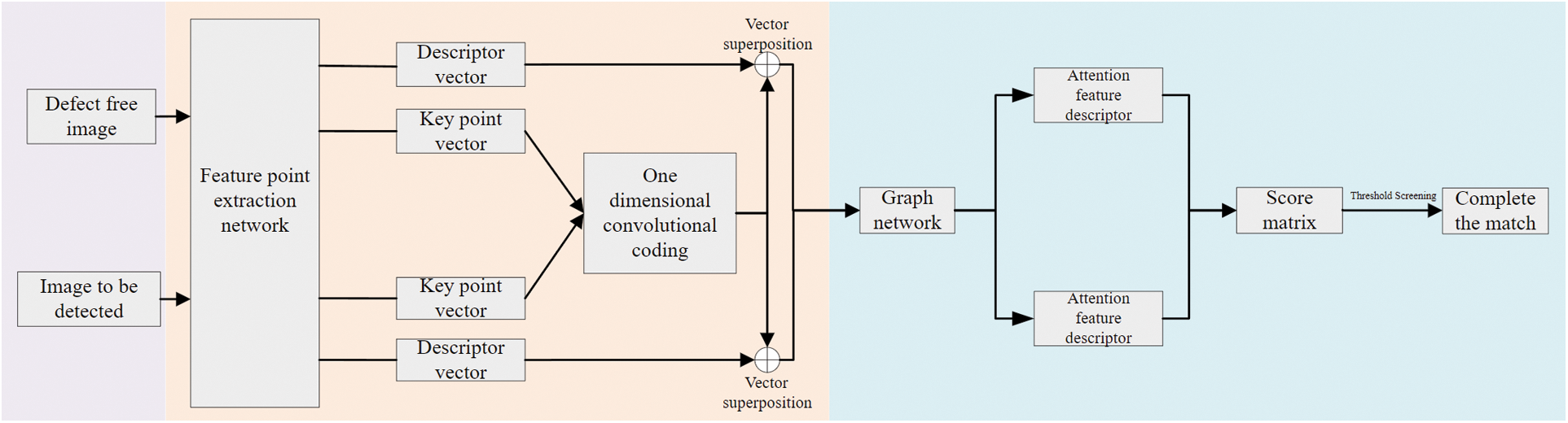
Figure 4: Matching flow chart. To extract the defects, firstly, working out the key point vector and feature descriptor vector of positive samples and samples to be detected respectively through the feature points extraction network, and then matching them through the graph attention network. Finally, correcting the images and then making residual, the area that having differences are regarded as defects

4.1 Pretreatment

The defects of printed matter often appear in the complex background area. In the case of defects in complex background will influence the descriptors of key points, the pixel level matching may not be achieved by conventional feature points matching algorithms, so we adapt the deep learning algorithm for matching. Since the dimension of the key point vector k is lower than that of the feature descriptor vector d. In order to fuse the key points and the feature descriptors, the low dimensional key points are mapping to the same dimension R256, and the feature descriptor vectors mapping by multi-layer one dimensional convolutional coding. Then the feature descriptor vector is normalized to eliminate the dimensionless influence between the feature descriptor vector and the encoded key point vector. The normalized feature descriptor vector is concatenated with the coded key point vector to obtain zA and zB, zA represents the vector of image without defects and zB is the vector of image to be detected.

4.2 Self and Cross Attention Network

The preprocessed zA and zB are put into the graph attention network. Graph attention networks are divided into self attention network and cross attention network. At the beginning, inputs zA and zB are transformed into feature triples:

{queryi(k)=Wquery(k)zi(k)+bquery(k)[keyj(k)valuej(k)]=[WkeyWvalue](k)zj(k)+[bkeybvalue](k)(1)

The superscript (k) is the index of current layers and subscript i and j are the indexes of key points. In practical application, we use multi-head attention mechanism [30] to enhance the expression ability of the model. Fig. 5 shows the framework of the attention network. The feature triples are used as the input of self attention and cross attention graph network, and they are cycled many times to enhance the robustness of the results. After testing, for common complex background of printed matter, the four layers graph attention network may achieve good performance (two layers of self attention network and two layers of cross attention network). The equation of basic attention mechanism in graph network is:

z=softmax(query⋅keyTd)⋅value(2)

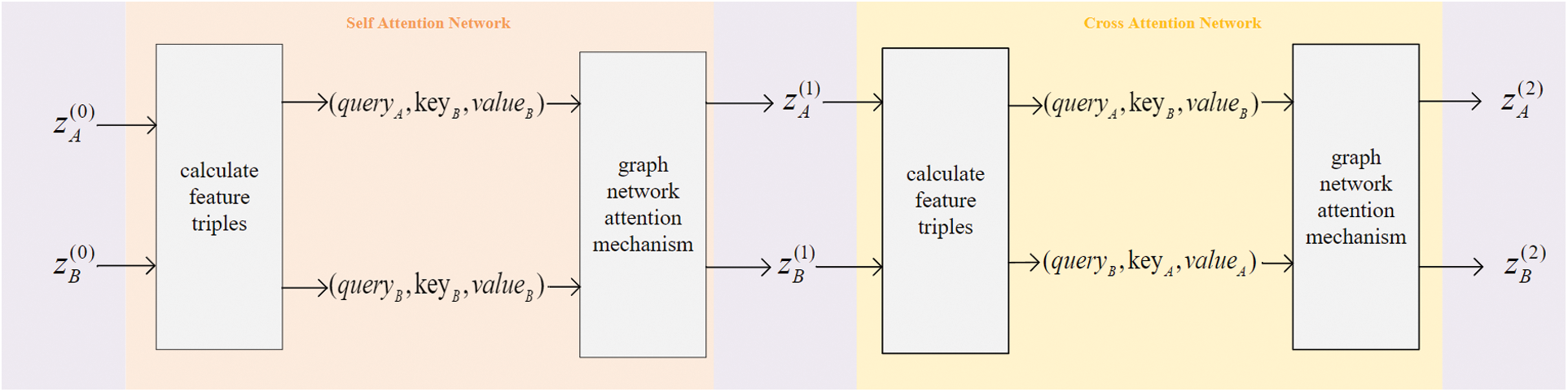
Figure 5: Graph Attention Network. The key, query, and value are computed as linear projections of deep features of the graph neural network and each layer has its own projection parameters, learned and shared for all key points of both images

Where d is the dimension of the query, which we use d=256 in this paper. We call the output of graph network as attention feature descriptor. The input feature descriptor vector is normalized to eliminate the dimensional influence, and the feature descriptor is re-calculated in the graph attention network. The output of the attention feature descriptor can judge the confidence of the prediction of the matching point by the vector value. We calculate the matching score matrix S∈Ra×b through the attention feature descriptors, and define an assignment matrix P∈[0,1]a×b. Where a and b are the numbers of local features in the images A and B.} Each term of the assignment matrix P represents the confidence corresponding to the feature points of two images, and the assignment matrix ∑i,jSi,jPi,j is obtained by maximizing the total score P:

Si,j=<ziA,zjB>0≤i≤a,0≤j≤b(3)

Where <⋅,⋅> is the inner product. For the feature points that have not been successfully matched, the method commonly used in traditional image matching is adopted. An additional row and column are set to store those feature points with poor matching performance, and the parameter z in the additional row and column is learnable.

S¯i,a+1=S¯b+1,j=S¯b+1,a+1=z∈R(4)

Assume that the additional rejection vector in the positive sample is α=[1aTa]T. Then the attention feature descriptor of the image to be detected will match the attention feature descriptor of the positive sample image or the additional rejection vector. The constraint of augmented matrix is:

P1N+1=α,PT1M+1=β(5)

The discrete distribution α and β in the augmented score matrix S can be regard as the optimal transmission problem. The Sinkhon algorithm [31] is widely used to solve the entropy regularization problem in the transmission problem. In order to solve the numerical instability of the Sinkhorn algorithm, we add the adjacent point algorithm [32] to solve the problem more efficiently. Finally, as shown in Eq. (6), the augmented part of the augmented score matrix is deleted to obtain the final matching score matrix.

P=P¯1:M,1:N(6)

According to the images set the appropriate threshold value and match successfully if the matching score is greater than the threshold value.

5  Experiments and Results

5.1 Experiment Setting

5.1.1 Dataset1

The images of the dataset used in this paper come from the industrial products, which is taken by the global shutter industrial camera. We worked closely with the organizers after the competition and got the raw data of the dataset. There are 16547 images from two different production lines, and the complete image size in Fig. 7 is 8192*2048 which is shown in Fig. 8. In order to facilitate the subsequent comparative experiments, the images are divided into different sizes. There are 7229 images are 128*128, and 8259 images are 256*256, and 1059 images are 512*512.

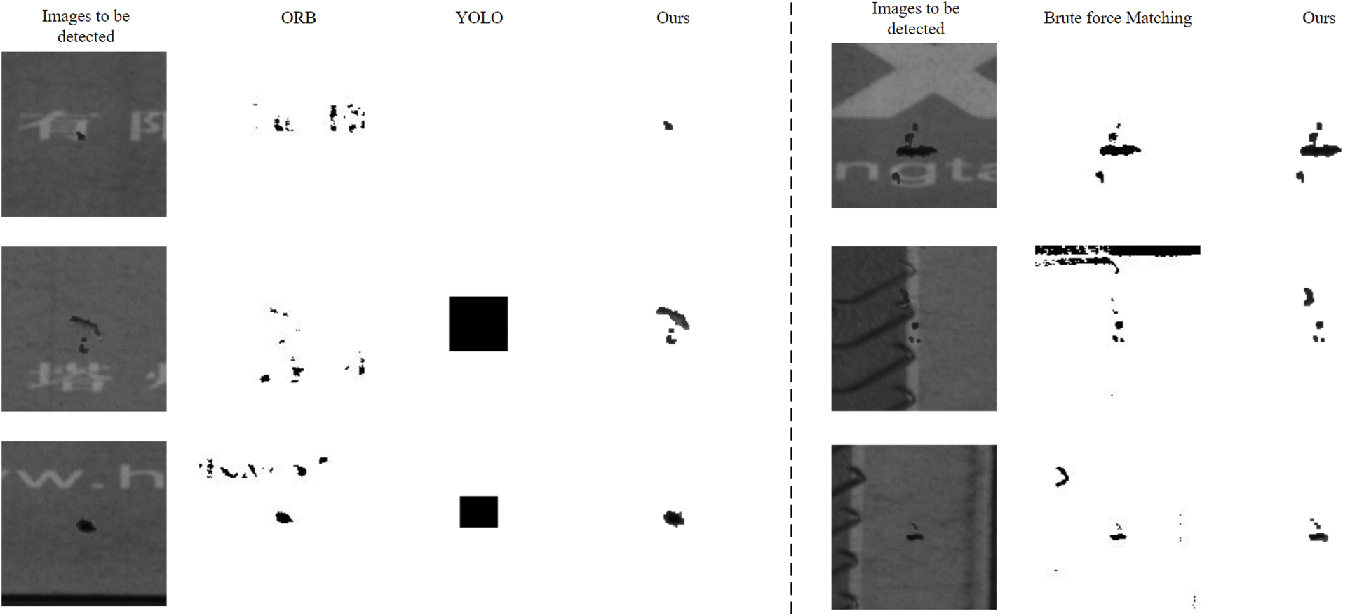
Figure 7: Contrast with different algorithms. The ORB algorithm can not solve the problem of complex print surface defects. The YOLO can not identify small defects (top row) and have many other probles in defect extraction, such as data annotations and rectangular box for detection. Compared with brute force(BF) algorithm(OpenCV) and our method, graph attention network can achieve pixel matching in complex environment

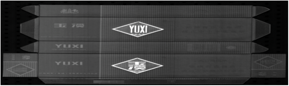
Figure 8: Full size positive sample image. The size of the image is 2048 × 8192

5.1.2 The Evaluation Criteria

The equations of Escape, overkill and mean of Intersection Over Union (mIOU) are:

escape=FNall(7)

overkill=FPall(8)

IOU=area(Rp∩Rgt)area(Rp∪Rgt)(9)

Where, the false positive(FP) represent the number of samples with wrong judgment in the positive example, the false negative(FN) represents the number of samples with wrong judgment in the negative example, and all represents the sum of positive and negative examples. Rgt represents the real defect area and Rp represents the predicted defect area, both of them are the set of pixels.

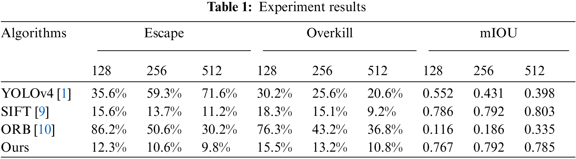
5.2 Analysis of Experimental Result

We compared our algorithm with the traditional image detection and deep learning algorithms. We randomly selected 10000 images as the training set of YOLO and the proportion of images of different size are nearly the same, and the remaining images as the test set. The backbone of YOLO is CSPDarknet53 network, which is much deeper and larger than VGG network used in ours. Tab. 1 shows the evaluation criteria with different algorithms. Because most of the target detection algorithms are based on rectangular box for labeling and detection, and defects with irregular edges will lead to overkill to a certain extent. On the other hand, most object detection algorithms fail to correctly label unmarked defect types as well as tiny defects in high-resolution images, resulting in an increase in the rate of missed detection. In the image of 128*128 size, the defect area is relatively large, while in the image of 1024*1024 size and only relatively obvious defects can be detected.

The traditional ORB algorithm [10] can not match the complex background of printed surface correctly. Only if the number of feature points is increased in large size images and the matching effect can be improved slightly. A large number of experiments show that our algorithm is superior to all the common image matching algorithms. Fig. 6 shows the result of defect extraction and the effect compared to the traditional algorithms.

5.2.1 Performance Analysis of Key Point Extraction Network

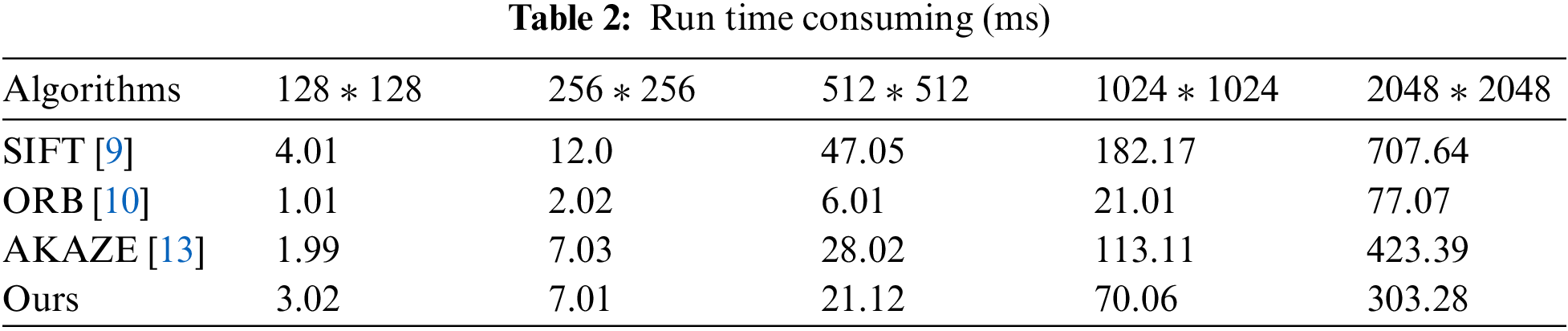
We compared the key point extraction network with the traditional algorithm. The experimental results are shown in Tab. 2, which respectively show the time (milliseconds) taken by different algorithms to extract key points from images of different size. To ensure fairness, the cost time here is the time of extracting key points from one image and do not include the time of matching.

5.2.2 Performance Analysis of Graph Attention Network

The graph attention network designed in this paper is compared with traditional brute force matching algorithm. The experimental results are shown in Tab. 3, and the matching results in different production lines are shown in Fig. 6. The brute force matching algorithm used is based on OpenCV3.4. If the positive samples and test samples come from different production line will case the problem of deviation because of different camera positions and so on. The experimental results show that for images obtained from the same production line, the performance of the graph attention network is similar to the brute force matching algorithm, and the performance of the graph attention network is better than that of the brute force matching algorithm for images obtained from different production lines.

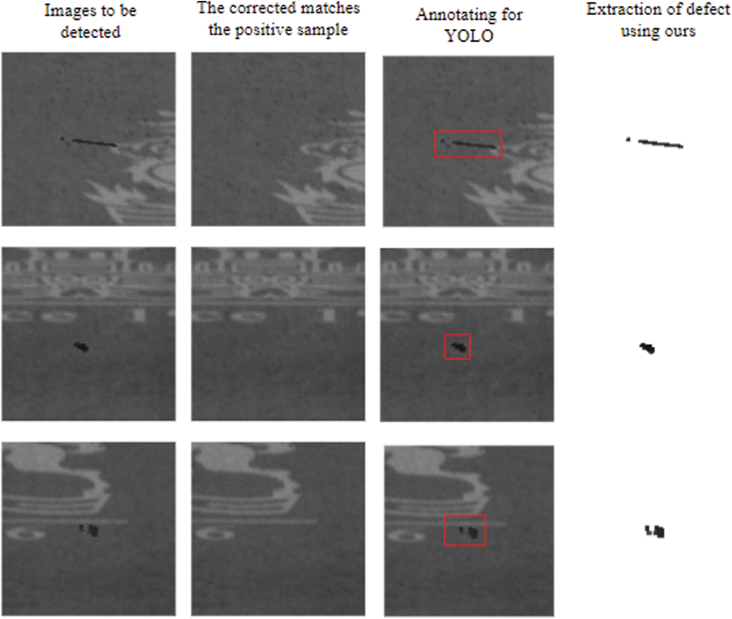
Figure 6: Actual effect of defect extraction. Because of the limitation of anchor, YOLO can not extract the defects in pixel level. All the images to be detected are from the actual industrial production environment

6  Summary

For a long time, the detection and extraction of products surface defects has been a hot issue in the industry. Nowadays, defect detection of a large number of products still relies on traditional image processing algorithms, and researchers need to design algorithms for specific products. On the one hand, most of the current defect detection algorithms are based on object detection of deep learning, which requires manual annotation of a large number of datasets, and the real-time performance is poor. On the other hand, unsupervised learning such as GAN and VAE require a large number of samples and can only deal with surfaces with relatively simple or repetitive texture. Our defect extraction algorithm based on positive samples has been tested on actual industrial datasets, and has achieved good results and meet the needs of manufacturers. Compared with SIFT algorithm, it has higher speed and accuracy. The defect extraction algorithm based on ours can also help label the datasets and save a lot of manpower.

Our algorithm had got excellent results in the finals of “The Frist ZhengTu Cup on Campus Machine Vision AI Competition” and we are working with the company to industrialize the algorithm. To improve the processing speed without changing the performance, we will compress and prune the model. This is one of the key issues that we are studying further.

Funding Statement: This work is supported by the National Natural Science Foundation of China (61976028,61572085, 61806026,61502058).

Conflicts of Interest: The authors declare that they have no conflicts of interest to report regarding the present study.

1Download address of competition dataset: http://focusight.marsbigdata.com

References

 1.  A. Bochkovskiy, C. Wang and H. Liao, “YOLOv4: Optimal speed and accuracy of object detection,” 2020. [Online]. Available: https://arxiv.org/abs/2004.10934. [Google Scholar]

 2.  Z. Cai and N. Vasconcelos, “Cascade r-cnn: Delving into high quality object detection,” in Proc. of The IEEE Conf. on Computer Vision and Pattern Recognition, Salt Lake City, Utah, pp. 6154–6162, 2018. [Google Scholar]

 3.  Z. Zhao, B. Li and R. Dong, “A surface defect detection method based on positive samples,” in Pacific Rim Int. Conf. on Artificial Intelligence, Cham, Barcelona, Spain, Springer, pp. 473–481, 2018. [Google Scholar]

 4.  S. Kcay, A. Atapour-Abarghouei and T. P. Breckon, “Ganomaly: Semi-supervised anomaly detection via adversarial training,” in Asian Conf. on Computer Vision, Cham, Springer, pp. 622–637, 2018. [Google Scholar]

 5.  G. Hu, J. Huang, Q. Wang, J. R. Li and Z. J. Xu, “Unsupervised fabric defect detection based on a deep convolutional generative adversarial network,” Textile Research Journal, vol. 90, no. 3-4, pp. 247–270, 2020. [Google Scholar]

 6.  T. Schlegl, P. Seeböck, S. M. Waldstein, U. Schmidt-Erfurth and G. Langs., “Unsupervised anomaly detection with generative adversarial networks to guide marker discovery,” in Int. Conf. on Information Processing in Medical Imaging, Cham, Springer, pp. 146–157, 2017. [Google Scholar]

 7.  S. Mei, H. Yang and Z. Yin, “An unsupervised-learning-based approach for automated defect inspection on textured surfaces,” IEEE Transactions on Instrumentation and Measurement, vol. 67, no. 6, pp. 1266–1277, 2018. [Google Scholar]

 8.  X. Tao, D. Zhang, W. Ma, X. Liu and D. Xu, “Automatic metallic surface defect detection and recognition with convolutional neural networks,” Applied Sciences, vol. 8, no. 9, pp. 1575, 2018. [Google Scholar]

 9.  P. C. Ng and S. Henikoff, “SIFT: Predicting amino acid changes that affect protein function,” Nucleic Acids Research, vol. 31, no. 13, pp. 3812–3814, 2003. [Google Scholar]

10. E. Rublee, V. Rabaud, K. Konolige and G. Bradski, “ORB: An efficient alternative to SIFT or SURF,” in 2011 Int. Conf. on Computer Vision, Barcelona, Spain: IEEE, pp. 2564–2571, 2011. [Google Scholar]

11. H. Bay, A. Ess, T. Tuytelaars and L. Van Gool, “Surf: Speeded-up robust features,” Computer Vision and Image Understanding, vol. 110, no. 3, pp. 346–359, 2008. [Google Scholar]

12. C. Wu, “A GPU implementation of scale invariant feature transform (SIFT),” 2007. [Online]. Available: http://www.cs.unc.edu/~ccwu/siftgpu/. [Google Scholar]

13. E. Rosten and T. Drummond, “Machine learning for high-speed corner detection,” in European Conf. on Computer Vision, Berlin, Heidelberg, Springer, pp. 430–443, 2006. [Google Scholar]

14. C. B. Choy, J. Y. Gwak, S. Savarese and M. Chandraker, “Universal correspondence network,” in Advances in Neural Information Processing Systems, Barcelona, Spain, pp. 2414–2422, 2016. [Google Scholar]

15. K. M. Yi, E. Trulls, V. Lepetit and P. Fua, “Lift: Learned invariant feature transform,” in European Conf. on Computer Vision, Cham, Springer, pp. 467–483, 2016. [Google Scholar]

16. Y. Ono, E. Trulls, P. Fua and K. M. Yi, “LF-Net: Learning local features from images,” in Advances in Neural Information Processing Systems, Montréal Canda, pp. 6234–6244, 2018. [Google Scholar]

17. D. DeTone, T. Malisiewicz and A. Rabinovich, “Superpoint: Self-supervised interest point detection and description,” in Proc. of the IEEE Conf. on Computer Vision and Pattern Recognition Workshops, Salt Lake City, Utah, pp. 224–236, 2018. [Google Scholar]

18. X. R. Zhang, W. F. Zhang, W. Sun, X. M. Sun and S. K. Jha, “A robust 3-D medical watermarking based on wavelet transform for data protection,” Computer Systems Science & Engineering, vol. 41, no. 3, pp. 1043–1056, 2022. [Google Scholar]

19. X. R. Zhang, X. Sun, W. Sun, T. Xu and P. P. Wang, “Deformation expression of soft tissue based on BP neural network,” Intelligent Automation & Soft Computing, vol. 32, no. 2, pp. 1041–1053, 2022. [Google Scholar]

20. I. E. Rube' and S. Alsharif, “Keypoint description using statistical descriptor with similarity-invariant regions,” Computer Systems Science and Engineering, vol. 42, no. 1, pp. 407–421, 2022. [Google Scholar]

21. S. Balammal Geetha, R. Muthukkumar and V. Seenivasagam, “Enhancing scalability of image retrieval using visual fusion of feature descriptors,” Intelligent Automation & Soft Computing, vol. 31, no. 3, pp. 1737–1752, 2022. [Google Scholar]

22. T. A. Al-Shurbaji, K. A. AlKaabneh, I. Alhadid and R. Masa’deh, “An optimized scale-invariant feature transform using chamfer distance in image matching,” Intelligent Automation & Soft Computing, vol. 31, no. 2, pp. 971–985, 2022. [Google Scholar]

23. M. A. Fischler and R. C. Bolles, “Random sample consensus: A paradigm for model fitting with applications to image analysis and automated cartography,” Communications of the ACM, vol. 24, no. 6, pp. 381–395, 1981. [Google Scholar]

24. P. H. S. Torr and A. Zisserman, “MLESAC: A new robust estimator with application to estimating image geometry,” Computer Vision and Image Understanding, vol. 78, no. 1, pp. 138–156, 2000. [Google Scholar]

25. J. W. Bian, W. Y. Lin, Y. Matsushita, Y. Yeung, S. K. Nguyen et al., “Gms: Grid-based motion statistics for fast, ultra-robust feature correspondence,” in Proc. of the IEEE Conf. on Computer Vision and Pattern Recognition, Honolulu, Hawaii, pp. 4148–4190, 2017. [Google Scholar]

26. P. E. Sarlin, D. DeTone, T. Malisiewicz and A. Rabinovich, “Superglue: Learning feature matching with graph neural networks,” in Proc. of the IEEE/CVF Conf. on Computer Vision and Pattern Recognition, Seattle, Washington, pp. 4938–4947, 2020. [Google Scholar]

27. K. Simonyan and A. Zisserman, “Very deep convolutional networks for large-scale image recognition,” 2014. [Online]. Available: https://arxiv.org/abs/1409.1556. [Google Scholar]

28. W. Shi, J. Caballero, F. Huszár, J. Totz, A. P. Aitken et al., “Real-time single image and video super-resolution using an efficient sub-pixel convolutional neural network,” in Proc. of the IEEE Conf. on Computer Vision and Pattern Recognition, Las Vegas, Nevada, pp. 1874–1883, 2016. [Google Scholar]

29. R. Keys, “Cubic convolution interpolation for digital image processing,” IEEE Transactions on Acoustics, Speech, and Signal Processing, vol. 29, no. 6, pp. 1153–1160, 1981. [Google Scholar]

30. C. Tao, S. Gao, M. Shang, W. Wu, D. Zhao et al., “Get the point of my utterance! learning towards effective responses with multi-head attention mechanism,” in Int. Joint Conf. on Artificial Intelligence, Stockholm, Sweden, pp. 4418–4424, 2018. [Google Scholar]

31. M. Cuturi, “Sinkhorn distances: Lightspeed computation of optimal transport,” Advances in Neural Information Processing Systems, vol. 26, pp. 2292–2300, 2013. [Google Scholar]

32. Y. Xie, X. Wang, R. Wang and H. Zha, “A fast proximal point method for computing wasserstein distance,” Uncertainty in Artificial Intelligence, Toronto, Canada, vol. 115, pp. 433–453, 2020. [Google Scholar]

This work is licensed under a Creative Commons Attribution 4.0 International License, which permits unrestricted use, distribution, and reproduction in any medium, provided the original work is properly cited.