DOI:10.32604/cmc.2022.027058
| Computers, Materials & Continua DOI:10.32604/cmc.2022.027058 | |
| Article |
Forecasting Mental Stress Using Machine Learning Algorithms
1Department of Software Engineering, Daffodil University, Dhaka, Bangladesh
2Collage of Computer Science and Information System, University of Najran, Najran, Saudi Arabia
3Department of Computer Science and Engineering, Khwaja Yunus Ali University, Sirajganj 6751, Bangladesh
*Corresponding Author: Abdulwahab Alazeb. Email: afalazeb@nu.edu.sa
Received: 10 January 2022; Accepted: 08 March 2022
Abstract: Depression is a crippling affliction and affects millions of individuals around the world. In general, the physicians screen patients for mental health disorders on a regular basis and treat patients in collaboration with psychologists and other mental health experts, which results in lower costs and improved patient outcomes. However, this strategy can necessitate a lot of buy-in from a large number of people, as well as additional training and logistical considerations. Thus, utilizing the machine learning algorithms, patients with depression based on information generally present in a medical file were analyzed and predicted. The methodology of this proposed study is divided into six parts: Proposed Research Architecture (PRA), Data Pre-processing Approach (DPA), Research Hypothesis Testing (RHT), Concentrated Algorithm Pipeline (CAP), Loss Optimization Stratagem (LOS), and Model Deployment Architecture (MDA). The Null Hypothesis and Alternative Hypothesis are applied to test the RHT. In addition, Ensemble Learning Approach (ELA) and Frequent Model Retraining (FMR) have been utilized for optimizing the loss function. Besides, the Features Importance Interpretation is also delineated in this research. These forecasts could help individuals connect with expert mental health specialists more quickly and easily. According to the findings, 71% of people with depression and 80% of those who do not have depression can be appropriately diagnosed. This study obtained 91% and 92% accuracy through the Random Forest (RF) and Extra Tree Classifier. But after applying the Receiver operating characteristic (ROC) curve, 79% accuracy was found on top of RF, 81% found on Extra Tree, and 82% recorded for the eXtreme Gradient Boosting (XGBoost) algorithm. Besides, several factors are identified in terms of predicting depression through statistical data analysis. Though the additional effort is needed to develop a more accurate model, this model can be adjustable in the healthcare sector for diagnosing depression.
Keywords: Depression analysis; mental health; machine learning; model deployment; XGBoost; ROC-AUC
According to the World Health Organization, about 264 million people worldwide suffer from depression. Each year, depression results in a substantial number of suicides, making suicide one of the leading causes of death among adolescents [1,2]. Besides, the National Institute of Mental Health (NIMH), 7.1% of American adults had a major depressive episode in 2017, with young people being the most severely affected [3,4]. According to the Nature Scientific Report, the 40% age of people experiencing symptoms of depression and anxiety has rapidly surged amid the Covid-19 outbreak. For the case of UK adults, the total rate of depression was 10% before the pandemic, but during the Covid-19 pandemic, the rate was enhanced from 10% to 19%. It was also found that the anxiety rate dramatically increased from 11% to 42% during the outbreak.
Again, the American Psychological Association (APA), primary care physicians are frequently asked to identify mental problems such as depression without proper training in how to treat them [1]. According to their estimates, patients’ psychological issues account for 70% of primary care visits. A physician treats more than 80% of patients with symptoms for which no diagnosis has been made. Only 10% of people seek help from a mental health expert [5,6]. Patients are not receiving the treatment they require, as 70% of people with depression go untreated. In a research published in JAMA, doctors compared patient outcomes, cost of care, and other factors between individuals who received more overt mental health diagnoses and treatment during routine doctor visits against those who did not [7]. Costs decreased, health care services were better utilized, patient outcomes improved, primary care doctor visits decreased, treatment interventions were started sooner, and hospital and emergency care visits decreased for patients who received mental health intervention [8]. This research aims to collect information about people typically found in a patient’s medical record to forecast depression. As stated in the previous study, many clinics or doctors may find it impossible to provide integrated mental health treatments. Having standard services where patients are constantly screened for mental health disorders and treatment is tightly integrated with teams of physicians, and psychological professionals can be costly, require a lot of training, require participation from many individual doctors who may feel overwhelmed, and may also be impossible in certain areas due to logistical issues.
The primary objective of this research is to predict who might have depression using machine learning and data that would ordinarily be in a patient’s medical file in a method that requires very little human interaction from clinicians and has lower time and money expenses. Patients suspected of having depression may be referred directly to mental health providers in their area who accept their health insurance. The patient’s file might also be highlighted to notify medical personnel when they have a doctor’s appointment, prompting doctors to begin dialogues with patients. At the absolute least, patients might be offered information and tools directly to encourage them to take action on their behalf. Furthermore, the following contributions have been assured in this research work: Firstly, applying several traditional machine learning techniques to measure the effectiveness while working on detecting the mental depression. Secondly, a software integrating pipeline has been interpreted through which researchers will understand how the machine learning model can be deployed and make them into the production level. Thirdly, A Comprehensive pipeline has been interpreted where several machine learning algorithms have been applied and identified the robust model using the model evaluation indicators. Eventually, hypothesis testing approaches have been explained, including loss optimization measurements, which will positively impact the research community to make a clinical model for predicting mental stress or depression.
Besides, we have applied various machine learning techniques and analyzed the data to discover insights regarding mental depression. In our investigation, we have seen that most of the depression is related to the four significant factors: Demographic, Medical Conditions, Occupation and Alcohol Use. Our experimental result would be a benchmark to the research community because it will be easy to determine the factors that lead to the development of depression. At the same time, by following the classification reports, it can be figured out the optimized model that should be considered while working on forecasting mental depression.
This study is organized into five interconnected sections. In section two, the literature review, we have reviewed the existing literature. In section three, the research dataset has been described. In section four, research methodology is illustrated. In section five, we have discussed the results and the corresponding relevant comparison. Finally, section six concludes the paper with future recommendations.
AlSagri et al. 2020 [9] objective is to identify whether a user is suffer from depression based on the analysing the tweets information. At the initial phase, data preparation, features extraction and various modules were used to measurement the data in terms of making a classifier. It is not be mentioned that in order to reduce the overfitting issues, the models were trained through 10-fold cross-validation technique and tested with the experimental dataset. In addition, Term frequency- Inverse document frequency (TF-IDS) was applied to compute the weight of the each words. Again, after pre-processing, and features extraction, Decision tree classifier and Support vector machine algorithms were used. Sampson et al. 2021 [10] conducted a study by following some steps-a Classification tree for incident depression was applied during follow-up among men (n 1/4 1951). Then, a Variable importance plot from a 10-fold cross-validation random forest was performed for incident depression during follow-up among men with no missing data (n 1/4 1409). Lastly, a Variable importance plot from a 10-fold cross-validation random forest was executed for incident depression during follow-up among women with no missing data (n 1/4 251).
Ramalingam et al. [11] performed preprocessing steps, then applied feature extraction with some techniques. After that, in the training phase, the SVM algorithm was used for making a classifier, and, eventually, depression and non-depression stages of individuals were predicted. In the case of textual inputs from various social media posts, the algorithm attempts to determine the text’s possible and probabilistic meanings through active and passive construction of all grammatical and general features of the text, as well as using semantic algorithms to determine the user’s emotion in the case of depression analysis. Ramalingam et al. [11] used different data types like text, speech, and image. In image analysis, a 2D feature vector is used to hold the features of each array of images broken into several different fragments so that each individual part of the image can be divided and studied separately. The process of classification was performed with some steps. The system attained an average detection accuracy of 82.2% for males and 70.5% for females using this method.
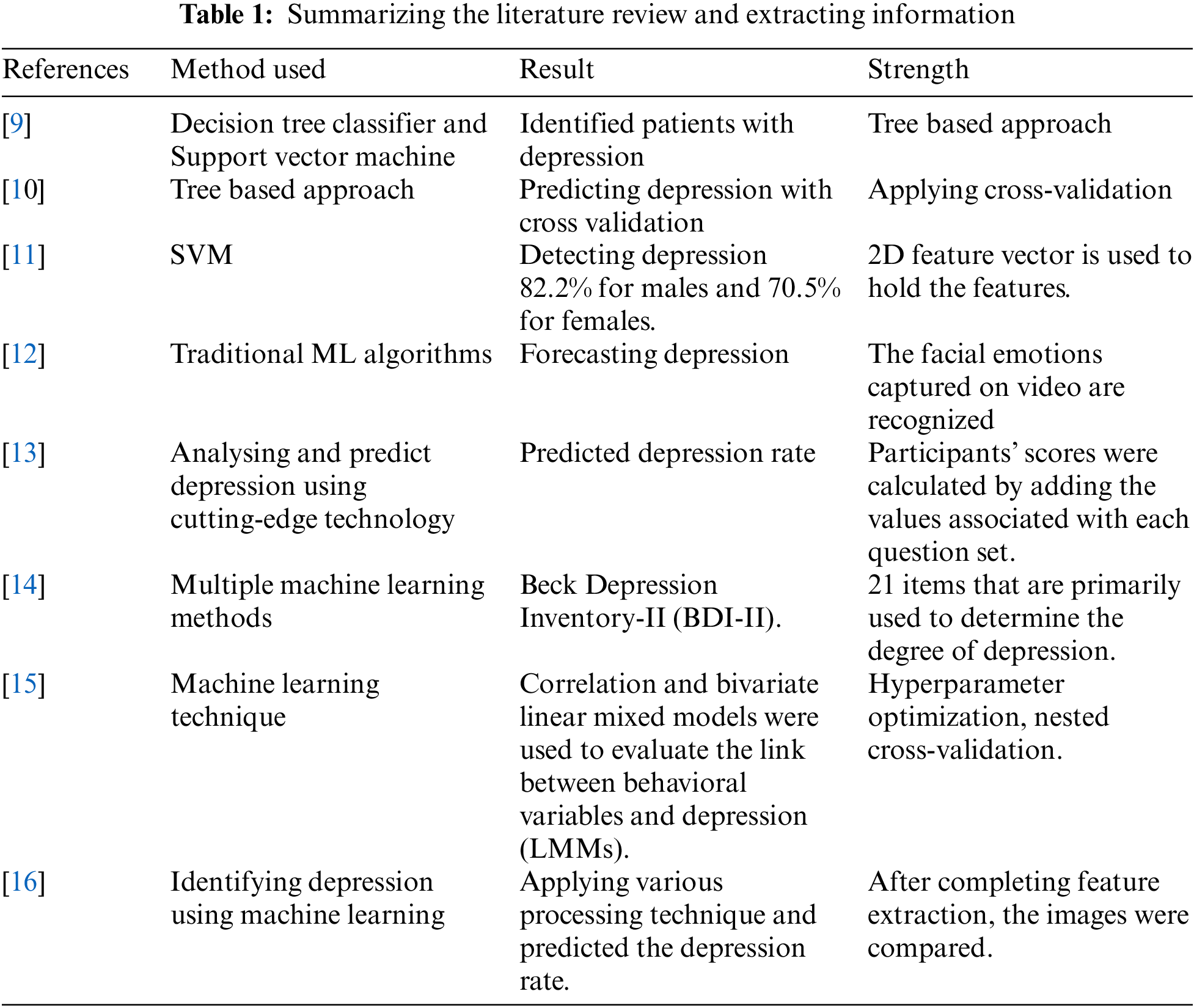
Narayanrao et al. [12] researched on analyzing the machine learning algorithms for forecasting depression. Videos of the general public are recorded and utilized as input for identifying depression [12]. The facial emotions captured on video are recognized—besides, the expression changes depending on the poses, lighting, person, viewpoint, and sensors. As a result, encoding information to detect depression is a complex undertaking. Following the collection of the dataset, a statistical model is created, trained, and modified as needed to produce accurate results. The model is developed and predicted on top of the concentrated dataset. Priya et al. [13] conducted a study towards analysing and predict depression, and stress for employed and unemployed individuals across various communities by applying some stress scale questionnaire. The responses of the participants were encoded using numeric values ranging from 0 to 3, and the participants’ scores were calculated by adding the values associated with each question set. The training and test sets were separated in a 70:30 ratio, representing the training and test sets, respectively. Zhao et al. [14] concentrated evaluating multiple machine learning methods for measuring the depression state of Chinese recruits applying the Beck Depression Inventory-II (BDI-II). The BDI contains 21 items that are primarily used to determine the degree of depression. Pessimism, suicidal thoughts, sleep difficulties, and social isolation are all symptom categories that each item corresponds to. The BDI assesses the severity of depression symptoms, which range from none to highly severe, divided into four stages, each with a value of 0–3. Asare et al. [15] investigated the potential of anticipating depression by an analysis of human behavior. Over an average of 22.1 days, an exploratory longitudinal study with 629 participants was conducted using smartphone data sets and self-reported eight-item Patient Health Questionnaire (PHQ-8) depression assessments (SD 17.90; range 8–86). Correlation and bivariate linear mixed models were used to evaluate the link between behavioral variables and depression (LMMs). To predict sorrow, we used five supervised machine learning (ML) techniques, including hyperparameter optimization, nested cross-validation, and imbalanced data treatment. In [16], Usman et al. tried to predict depression by a machine learning approach. To detect depression from facial images, firstly, they have taken input images, then pre-processed. After completing feature extraction, they compared images. After that, output decisions in labels were figured out. Tab. 1 shows the corresponding summary of the research gap analysis of the existing solution.
The National Health and Nutrition Examination Survey of the Centers for Disease Control and Prevention provided the dataset for this study. This data set contains a wealth of health information on a random sample of the American population and is released every two years. The data can be found in [17]. Between 2005 and 2018, 36259 adults in the United States provided data for this study. Only data consistent between years was used and data that might reasonably be found in a patient’s medical file. It’s ideal to utilize as little data as possible while still producing accurate projections. It would catch more patients who don’t have comprehensive medical histories and relieve providers of the burden of collecting so much information. The PHQ-9 depression screening questionnaire, given to all NHANES participants, was used to set the target. According to the study, with a threshold score of 10 or higher, this screening measure has an 88% specificity and sensitivity for major depression. Based on their scores on the screening test, 5 people were classified as “depressed” or “not depressed,” with a score of 10 or higher signifying “depression.” This research aimed to build a number of model types and compare and contrast them to see which ones performed the best. The modelling endeavour began with simpler models and advanced to more complex ones. Although we have used several features to predict depression, the significant parameters listed are responsible for mental depression, such as blood_transfusion, arthritis, heart_failure, heart_disease, heart_attack, thyroid_problem_currently, thyroid_problem_onset, Rx_days_RALOXIFENE, BMI, pulse, weight and height.
The proposed methodology is classified into four significant phases. In the initial phase, the data management mechanism will be enumerated with the hypothesis and data modeling. In the second phase, the experimental setup of the predictive model will be constructed with experimental setup and model analysis. In the architecture section, the different conventional classifiers will be adopted. In the third phase, model testing will be placed through the evaluation and identification of significant factors. After that, a mechanism of comparative analysis of the models will be interpreted along with the way of connecting the whole software integration. In the final phases, the proposed architecture will present the result of prediction on mental pressure and depression. Fig. 1 illustrates the architecture of this proposed research.
4.1 Proposed Research Architecture (PRA)
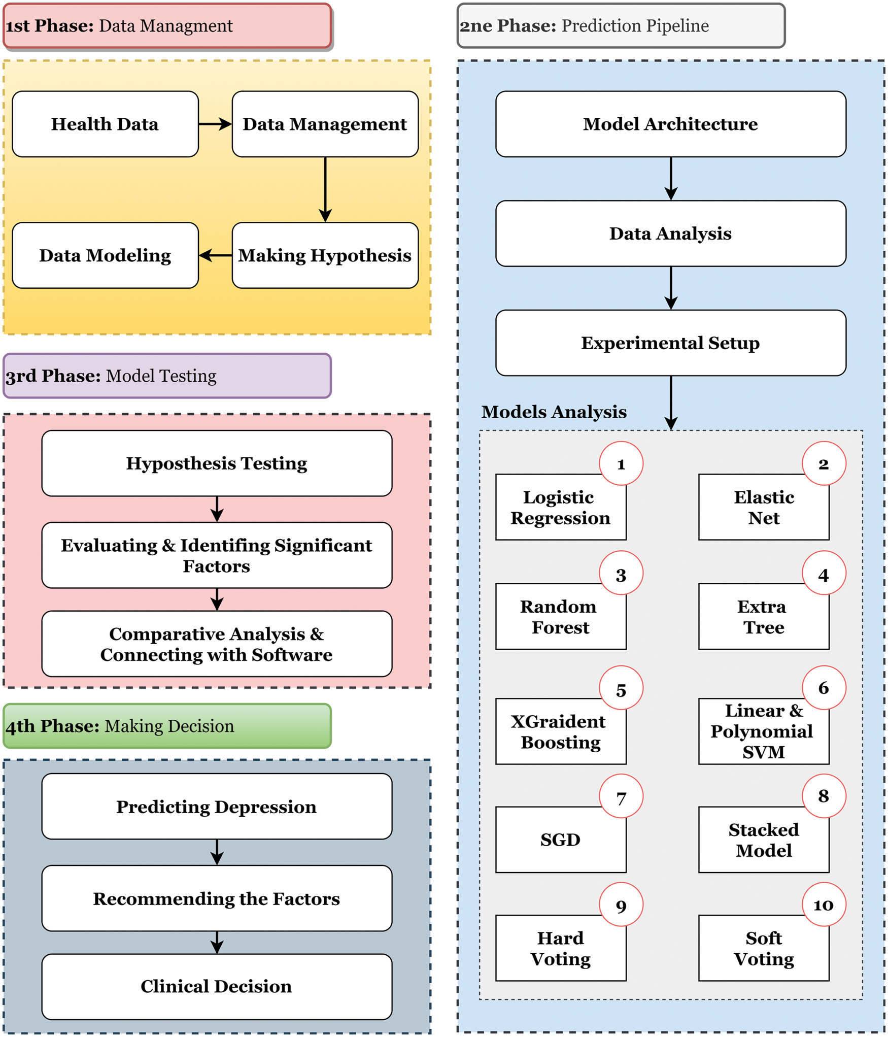
Figure 1: Demonstrating the proposed research architecture. The entire research has been conducted by following the four steps mentioned in the PRA starting from data management to model analysis
4.2 Data Preprocessing Approach (DPA)
Because raw data (data from the real world) is incomplete and cannot be passed via a model, it has been altered using a data mining technique. As a result, to obtain correct findings, the data has been preprocessed before being fed into a model. With the information in the dataset, the features have been investigated from both a statistical and a semantic standpoint. This procedure has been used with Normalisation, Attribute Selection, Discretisation, and Concept Hierarchy Generation. When working with vast amounts of data, analysis becomes more complicated if the data dimension is significant; however, the data reduction approach has been used to cope with enormous amounts of data. Besides, the Data Transformation technique and Encoding the categorical data are applied to the preprocessed dataset. Using this absolute data encoding method, the category variable is turned into binary variables (also known as dummy variables). For N categories in a variable, N binary variables are utilized in one-hot encoding. Dummy encoding is a slight advancement over one-hot encoding [18]. In computing, data transformation refers to the process of converting data from one format or structure to another. It is required for the majority of data integration and management operations, including data wrangling, data warehousing, and application integration.
4.3 Research Hypothesis Testing (RHT)
The hypothesis is a very obscure and complex part of the world of statistics. Simply put, a hypothesis is a hypothetical claim about a population. But this imaginary claim must be mathematically verifiable. Hypotheses can be of two types, e.g., Null Hypothesis and Alternative Hypothesis. The Null Hypothesis is a claim about the population that is initially considered to be true until it is proven false. H0 expresses the null hypothesis. Expression of null hypothesis may have =, <= or >= sign. On the other hand, if the null hypothesis is proved to be false, then another hypothesis is considered an alternative that is considered true; this hypothesis is called Alternative Hypothesis. HA expresses alternative hypotheses. Alternative hypotheses cannot contain expressions of null hypotheses (=, <= or >=). In that case, the expression of the alternative hypothesis may be ≠, >, <, etc. Hypothesis testing is the process of checking whether a hypothesis is correct. In Hypothesis Testing, we can whip up or accept any null hypothesis. When testing a hypothesis, the correct hypothesis may be considered incorrect, and the incorrect hypothesis may be considered correct. This type of error is called hypothesis testing error. This error can be of two types: Type I Error-When a true null hypothesis is rejected, it is called a Type I Error. Type II Error- When a false null hypothesis is not rejected, it is called Type II Error. Z test and t-test-we use z distribution when the value of population standard deviation is known, and such test is called z test. On the other hand, when the value of population standard deviation is unknown, we use t distribution, and such test is called t-test. The p-value is a probability value. When examining a hypothesis with a p-value, the null hypothesis is rejected if the significance (level of significance) is greater than the p-value. In contrast, if it is smaller than the p-value, the null hypothesis is not rejected. Nonetheless, Algorithm1 depicts the steps to test the hypothesis in p-value method. In addition to
where

4.4 Concentrated Algorithm Pipeline (CAP)
In this research work, 14 different machine learning algorithms were experimented on top of the dataset, e.g., Logistic Regression (LR), Elastic Net, Random Forest (RF), Extremely Randomized Trees Classifier, eXtreme Gradient Boosting (XGBoost), Linear Support Vector Machine (Linear SVM), Polynomial SVM, Stochastic Gradient Descent (SGD), Stacked Model, Non-Tree Stacked Model, Hard Voting Model, Soft Voting Model, Hard Voting Model (Non-tree) and Soft Voting Model (Non-tree). This is to say that the RF and Extremely Randomized Trees Classifiers are provided with satisfactory performance among the robust classifiers. In this section, the comprehensive interpretations have been delineated with their mathematical explanation.

Random Forest Model: Random Forest Algorithm is called Ensemble Learning which enhances model performance by using multiple learners. Random forests are made up of many trees or shrubs. Just as there are many trees in the forest, random forests also have many decision trees. The decision that most trees make is considered the final decision. Following the bagging, method does not affect the random forest outlier. It works quite well in both categorical and continuous data and does not require scaling the dataset. However, the following Algorithm 2 has been taken into consideration in order to make the Random Forest.
Extremely Randomized Trees Model: The Highly Randomized Trees Classifier (Extra Trees Classifier) is an ensemble learning technique that generates a classification result by aggregating the output of several de-correlated decision trees collected in a “forest.” ExtraTreesClassifier is a decision tree-based ensemble learning technique. As with RandomForest, ExtraTreesClassifier randomizes certain decisions and data subsets in order to avoid overlearning and overfitting. Extra Trees is similar to Random Forest in that it generates numerous trees and splits nodes randomly. Nonetheless, there are two significant differences: it does not bootstrap observations (that is, it samples without replacement), and nodes are split randomly rather than optimally. To summarize, ExtraTrees: Bootstrap=False generates several trees by default, meaning that it samples without replacement. To separate nodes, random splits among a random subset of the attributes presented at each node are used. Extra Trees’ randomness comes from the random splits of all observations, not from bootstrapping the data. Furthermore, sometimes precision is more important than a broad model. As a result, it provides Low Variance and, more importantly, feature significance.
4.5 Loss Optimization Stratagem (LOS)
The first two optimization strategies are described in this article: ensemble learning and frequent model retraining. The following sections clearly show the loss optimization techniques that have been utilized in this proposed research.
Ensemble Learning Approach (ELA): Implementing alternative models, either using the same method with different training data or using different algorithms with the same training data, typically results in varying levels of model accuracy, making one model less than ideal for performing a machine learning job. Multiple models are created and used by intelligently combining the findings of the models so that the overall accuracy is greater than the accuracy of any single model. Models for classification and regression are constructed using either homogeneous or heterogeneous approaches. The meta-model is then constructed using techniques such as bagging, boosting, and random forests.
Frequent Model Retraining (FMR): How can a model’s efficacy be assured once it has been deployed? There’s a good chance that once a model is deployed in the production environment, its accuracy will deteriorate with time, resulting in poor system performance. The machine learning model is in sync with the changing data. At regular intervals, the model is retrained by creating a training data set that comprises both historical and current data.
4.6 Model Deployment Architecture (MDA)
When a machine learning model’s insights are frequently made available to the people for whom it was designed, it can begin to offer value to an organization. Deployment is the process of taking a trained machine learning model and making its predictions available to users or other systems. This section illustrates a comprehensive pipeline that can be utilized to deploy the machine learning model, mainly predicting and analyzing the depression. Deploying the model into a server and generating a Representational state transfer (REST) API can be the key solution to make a communication protocol from which the software system can be transmitted the data. The detailed sequence and consequences are shown in Fig. 2.
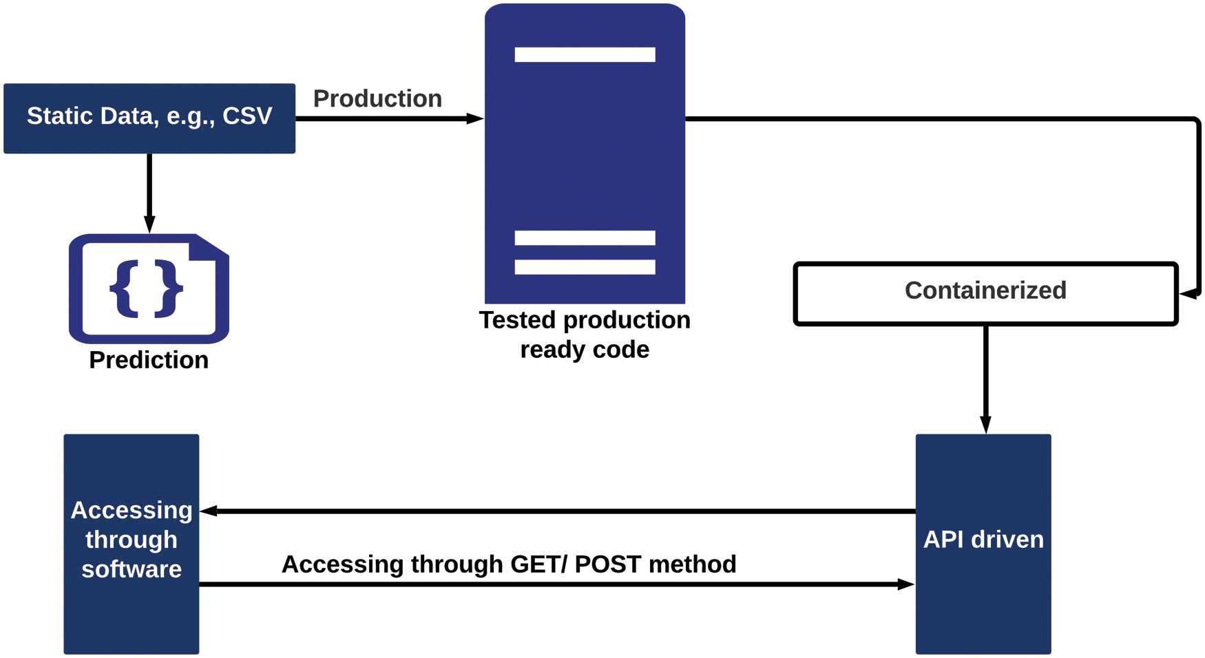
Figure 2: Initially, the static data will be forwarded through the production module and the data will be transmitted to the software system by accessing API driven components
5 Results, Observation and Discussions
5.1 Classification Report Interpretation (CRI)
In this research, several evaluation metrics are adopted to measure the performance of the suggested models. To illustrate, classification report, confusion matrix, cross-validation and ROC-AUC curve. A classification report is one of the metrics used to evaluate the performance of a classification-based machine learning model [19]. It summarizes the model’s precision, recall, F1 score, and support. It gives a more complete picture of the trained model’s overall performance. To interpret a classification report generated by a machine learning model, it is required to be familiar with all of the metrics included in the report. Moreover, Tab. 2 gives the information about the performance and efficacy recorded through the measurements and the concentrated algorithm to predict depression.

5.2 Classification Report Measurement
Grid search had no discernible effect on model performance [20]. By correctly categorizing 68% of those data, logistic regression excellently captures the sad class. It does a better job with people who aren’t depresed. With an AUC value of.82, the model can discriminate between the kinds quite well, meaning it can distinguish between the classes around 82% of the time. The elastic net model performs no better than when the Elastic net penalty is removed. Because it maximizes accuracy and selects the dominant class, the base model is terrible. The tuned model performs worse than the logistic regression in predicting the depressed class, but it performs better in predicting the non-depressed class. Many aspects of sleep, employment, and health issues are incorporated into the model. According to the AUC score, the model can roughly 81% of the time between classes, which is slightly worse than logistic regression. The fundamental model, once again, focuses on accuracy, which means it performs poorly because it only selects the majority class. Extra trees predict the depressed class better than the random forest, but not as well as logistic regression. Different trees are a better model than random forest, but inferior than logistic regression since recall is more essential than precision. The AUC is 0.81, which is the same as the random forest. So far, the best method for distinguishing between the two classes has been logistic regression. This model includes elements like work, sleep, and health concerns comparable to those found in random trees. The vanilla model outperforms the other tree models, which is surprising given the vanilla model’s poor performance. Although the base model is competitive with logistic regression, the tweaked model loses a lot of its capacity to correctly forecast the depressed class, which is the most crucial factor in this project. Surprisingly, the baseline model would perform worse than the adjusted model. Further, XGBoost features, such as the ability to employ certain optimizing functions for gradient descent, should be investigated. The tweaked model’s AUC is only 0.77, compared to 0.82 for the base model, which is the same as the logistic regression. Many of the aspects of prescriptions are different in the adjusted model than in the other tree-based models.
The tuned model performs similarly to the logistic regression model, but it has a 1% increase in the number of true negatives identified, making it a superior model. This model performs similarly to the base XGBoost model. The AUC score is still 0.82, which is only a little higher than the previous high. The tuned model is similar to the extra trees model, except it accurately classifies 1% of true negatives. On the other hand, accurate positive detection is worse than linear SVM or logistic regression models. The AUC value is 0.82, which is comparable to the top models, such as logistic regression. The gradient descent classifier significantly improved the model’s performance. Both tweaked models were successful in enhancing the correct classification of people who were depressed. Both models have an AUC of 0.82, but the model using standard scaled data is more accurate since it predicts the non-depressed class. However, despite being inferior at predicting the not depressed class, the model with the original preprocessing is 1% better at predicting the sad class. In both stacks of previous models, stacking did not enhance performance. The entire stack of models outperformed the non-tree models-only stack. The hard vote classifier, which used non-tree models solely, did the most incredible job of diagnosing depression. These models aren’t any more effective than logistic regression or the SGD classifier. Soft vote models performed worse than sophisticated vote models.
Overall, the SGD classifier employing standard scaling to prepare the data proved to be the best model. The SGD model that used the original scaling at the start of the notebook performed 1% better in the sad class but had a more severe drop in performance in the not depressed class. Though many models were more accurate than the best model in classifying the not depressed group, linear models, such as logistic regression, linear SVM, and SGD classifier, fared the best. In general, tree models do not appear to be well-suited to forecasting depression, although the extra trees model performed the best. The base model of XGBoost performed better than the tuned model, indicating that more research is needed to increase performance. It was complicated to characterize the depression category appropriately. Almost every model correctly identified over 80% of true negatives; however, the SGD classifier earned the highest %age of true positives captured at 72% utilizing the project’s initial preprocessing.
That’s a lot better than guessing and shows that this work is doable, but there’s still an opportunity for improvement, which might be accomplished with more experimenting. The better the models predicted the depressed class, the worse they predicted the non-depressed class. This research included a lot of experimentation; however, not everything was shown in this research due to space constraints. For example, this study was attempted with fewer features obtained and cleaned before modeling, but the models’ performance is significantly improved with the additional features. Modeling was also tested with two alternative resampling strategies to see whether they may increase performance by balancing SMOTENC and SMOTENC paired with under sampling. Neither of the resampling techniques worked to improve performance. The models trained on the resampled data performed significantly worse than those trained on the original unbalanced dataset and used the class weight parameter. The most impactful and least impactful features can be examined and studied using the coefficients from the SGD classifier models. The model with conventional scaling is the best overall, although it can be compared to the model with original preprocessing for comparison purposes. Then, using the complete dataset, some of the most important attributes can be replotted to look at trends.
In the instance of tree-based models, methods to run a classification report, create a confusion matrix, plot a ROC curve, and plot feature importance were built to evaluate model performance. Total accuracy will not be a valuable indicator of how well the model performs in the imbalanced classes. The ROC curve can be used to visually check whether a model can distinguish between the two classes [21]. Looking at the confusion matrix will be helpful you see how many depressed people the model is correctly detecting [22,23]. False positives are preferable to false negatives, so it’s better to label some people as depressed even if they aren’t because, at the worst, they’ll be directed to help they don’t need. Missing people with depression, on the other hand, would mean that the worst-case situation would be suicide. A modified F statistic will be used as the scoring object for the models, with recall weighted higher than precision. As a result, the models will focus on striking a balance between precision and recall, favoring recollection to reduce false negatives, and, as previously stated, prioritize precisely detecting those who have depression. This is a common medical test scoring technique [24]. The traditional F1 statistic is calculated as:
The F1 statistic equation is usually spelled down like this, although it may alternatively be stated as:
An F2 statistic, also known as a Fbeta statistic, was used to generate the scoring for this study. The F2 statistic is computed as follows:
When the F2 equation is examined, it can be seen that it simply replaces a 2 where there is ordinarily a 1. Technically, depending on the desired precision or recall weighting, an F0.5 statistic or an F3 statistic might be calculated. Precision has a greater impact on the final computation when the number is less than one. A number greater than one causes recall to have a greater impact on the final computation, which is why F2 was utilized in this study. Confusion Matrix, ROC-AUC Curve, and Loss Accuracy Measurement are some of the assessment metrics used to test our concentrated model [25]. To put it another way, a confusion matrix is an effective tool for evaluating classification models. It shows how well the model identified the classes using the data you providedp and misclassified lessons. The Receiver Operator Characteristic (ROC) curve is a tool for evaluating binary classification issues. A probability curve plots the TPR against the FPR at various threshold levels, allowing the signal to be distinguished from the noise. The AUC is a summary of the ROC curve that indicates the ability of a classifier to distinguish between classes [26]. The AUC measures how successfully a model can differentiate between positive and negative classifications. The greater the AUC, the better the model’s performance. When AUC equals 1, the classifier effectively distinguishes all Positive and Negative class points. When the classifier with an AUC of 0.5 is unable to distinguish between Positive and Negative class points, the classifier would predict all Negatives to be Positives and all Positives to be Negatives. The classifier predicts either a random or a constant class for all of the data points. As a result, the AUC score of a classifier determines how well it can distinguish between positive and negative classes as shown in Fig. 3.

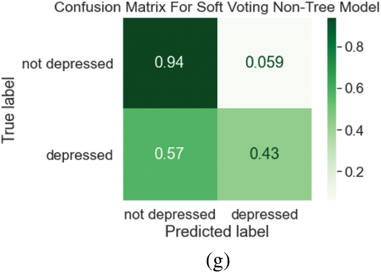
Figure 3: (a) Confusion matrix for random forest tuned model (b) ROC curve for random forest tuned model (c) confusion matrix for tuned polynomial SVM (d) ROC curve for tuned polynomial SVM (e) confusion matrix for extra tree classifier model (f) ROC curve for extra tree tuned model (g) confusion matrix for soft voting non-tree model
5.4 Exploratory Statistical Data Analysis (EDA)
This section depicts the exploratory statistical data analysis results based on the findings extracted from the dataset (ESDA). When all of the features in the dataset are plotted together, some appear to have a significant difference between those who are depressed and those who are not, while others seem to have little to no difference. By doing so, considerable information will have to the research community to identify the individual who is being depressed or not. The ESDA is categorized based on the specific information, especially the factors are shown to be responsible for depression. To put it more simply, we have explored the following aspects in order to find out the significant factors, e.g., Demographics, Medical Conditions, Body Measures, Blood Pressure, Cholesterol, Standard Biochemistry Profile, Blood Count, Occupation, Sleep Disorders, Physical Activity, Alcohol Use, Physical Functioning, Recreational Drug Use, Smoking, and Prescription Medications. Those who have trouble sleeping are four times more likely to be depressed than those who do not. The sleep hours of the depressed group are concentrated in a smaller range than those of the non-depressed group. Those who engage in moderate to vigorous physical activity in their leisure time have a lower risk of depression than those who do not. People who work jobs that demand moderate to vigorous physical activity have the same rate of depression as those who do not. In terms of physical functioning, the %age of persons who are depressed is higher among those who are suffering from a health problem. The health issues that cause the most depression include memory problems and birth abnormalities. In the case of recreational drug use, those who had used any of the drugs on the list were more likely to be depressed. The %age of those who had used heroin had the highest rate of depression. A higher rate of depression was seen among those who had completed a rehabilitation program. Smokers had more excellent rates of depression than nonsmokers, and those who smoked more frequently had a higher rate of depression than those who smoked less regularly. Smokers who are depressed start smoking at a younger age than non-depressed smokers. Those who have quit smoking and suffer from despair have documented fewer days since leaving. The number of drugs people take and the %age of people who are depressed are inextricably linked. However, concluding those entries is difficult because the highest values for the number of drugs are limited. For all of these medicines, there is an increase in the %age of persons who are depressed, with some of the additions being extremely significant, as in the case of Albuterol.
Factor 1—Demographics
In terms of Demographics, it is clear that females suffer from depression at a far higher rate than males. It is worth noting that those who have completed less education are more prone to be depressed. When looking at Fig. 4, it is clear that those who are divorced or separated have higher rates of depression. Married people, on the other hand, have the lowest rates of depression of any marital status. As household income grows, the %age of people who are depressed decreases, indicating a significant disparity in household income. Furthermore, throughout their middle years, melancholy persons appear to be more concentrated.
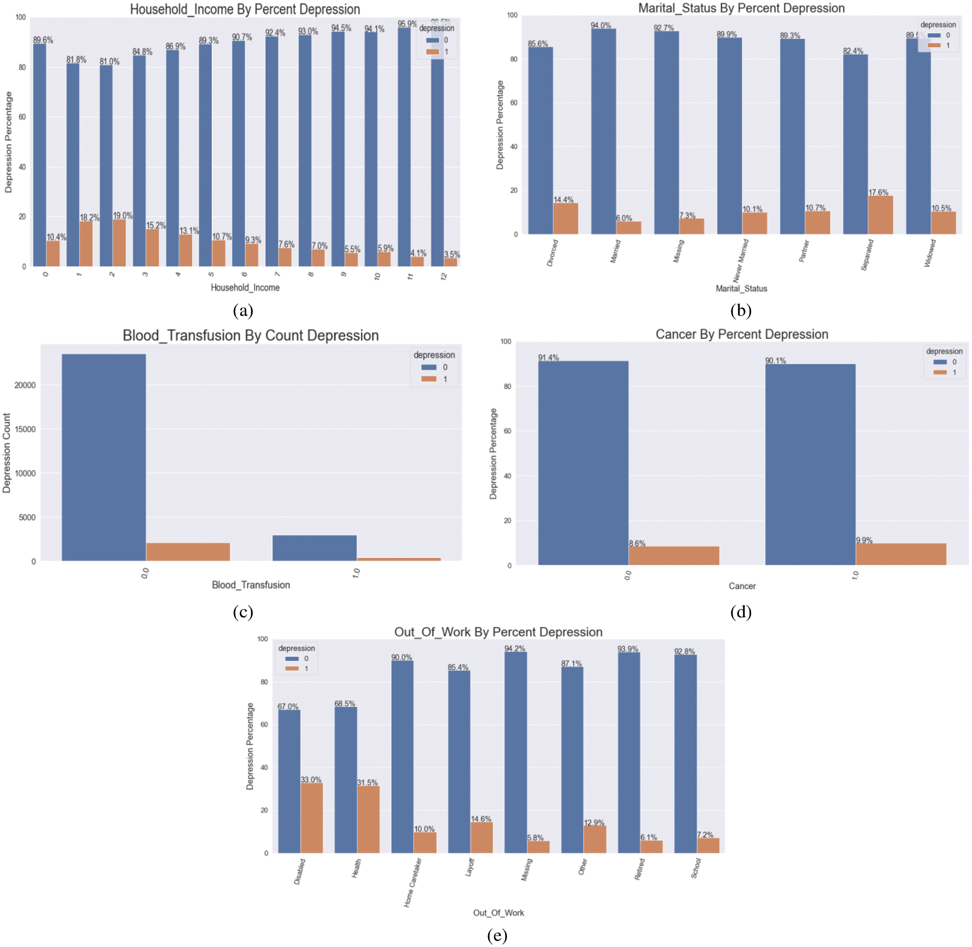
Figure 4: (a) Household income by % depression (b) marital status by % depression (c) representing blood transfusion by count depression (d) visualizing cancer by % depression (e) demonstrating depression regarding out of the work
Factor 2—Medical Conditions
People who have had a blood transfusion had a higher incidence of depression in this group. Unsurprisingly, any medical issue has a higher %age of persons who are depressed. There isn’t much of a difference when it comes to sad cancer patients vs. those who aren’t. However, because cancer types fluctuate, the prognosis and treatments available for a specific malignancy may factor. Surprisingly, none of the cancer types in our cohort had any episodes of depression. High fever has been linked to a higher rate of depression.
Factor 3—Occupation
In this dataset, those out of work due to illness or disability have a greater rate of depression. Those who have been laid off have a higher rate of depression than the general population. Those who are not depressed have been at their current work for an average of two years longer than those who are. Nonetheless, Fig. 4 graphically depicts the detailed sequences and consequences, with the essential elements displayed with relevant data.
Factor 4—Alcohol Use
Those who are not depressed have remained at their current work for an average of two years longer than those who are depressed. Those who did not suffer from depression drank more alcoholic beverages in the previous year than those who did.
5.5 Features Importance Interpretation
Compared to traditional scaling, the SGD model with original preprocessing includes more features and significant coefficients [27]. However, many of the same characteristics can be found on both lists of leading coefficients for both models [28]. The strenuous and moderate recreation options are also noteworthy. The preprocessed initial model caught up on individuals who don’t have as essential qualities as the usual scaling model gathered upon those who indulge in vigorous or moderate recreation. The clustering did not affect the typical scaling model, which had a 0 coefficient. The original processing only had a slight effect on the model. Could the cluster column have been hot encoded to have a more significant impact? Many different forms of cancer have little effect on either version of the SGD model. There were significant disparities in the %ages of depression amongst the various forms of cancer, as noted in the explore portion of this notebook. Many prescription-related elements do not influence either model, and none of the prescription-related features have been chopped into upper pieces. This is relatively surprising, given every prescription examined in the explore section had a more significant rate of those who were depressed who were taking the drug. Some of the variations were minor, but others were significant, leading one to believe that some drugs might significantly impact models. What we now know about depression explains some of the most significant factors influencing the model. For example, it was already indicated in the introduction that depression rates were higher in younger age groups. The model backs this up, as the negative coefficient value indicates that as people get older, they are less likely to fall into the depressing category, as predicted by the model. Another example is a history of sleeping problems. Changes in sleep patterns are a well-known symptom/sign of depression; therefore, it’s not surprising that this attribute would have an effect on the model. According to the model, the positive score indicates that those who have ever discussed sleeping problems with a doctor are more likely to be depressed. Some of the more impactful aspects, such as the citizenship function, come as a surprise. Citizens are less likely to feel depressed, according to the citizenship Citizen component of the first plot. Perhaps this has anything to do with non-citizens’ stress or the perks available to citizens. Both models had both recreational exercise qualities and a history of sleeping problems and sleep hours. In terms of the core elements, both models have a lot in common as shown Fig. 5. Tab. 3 shows the coefficients with the largest values according to the standard. Tab. 4 shows getting the coefficients with the highest values according to the original. Tab. 5 shows interpreting the top coefficients values.
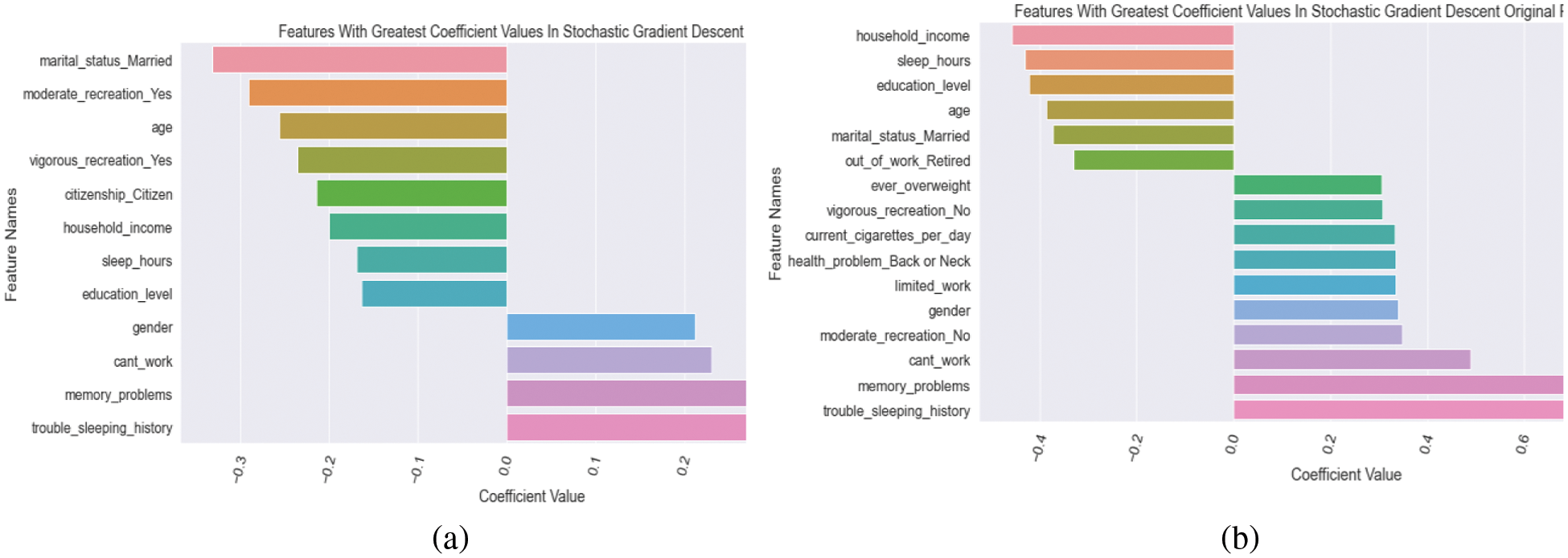
Figure 5: (a) plotting the top coefficients from the standard scaling model (b) Plotting the top coefficients from the initially processed model


After reviewing the literature, we have extracted some meaningful insights in terms of forecasting depression using various machine learning and deep learning techniques. It is noticeable that the decision tree model is thorough and follows logical processes; it can fail while recieving with new data. On the other hand, we have noticed that the SVM model achieves optimal accuracy metric combinations; it converts a highly non-linear classification problem into a linearly separable problem algorithm. The number of social media users is increasing day by day. Although it has several advantages, there are also huge demerits. Depression is interrelated to social media. It is also observed that applying machine learning techniques to identify depression was the primary objective of several studies conducted beforehand. Researchers frequently applied machine learning algorithms rather than deep learning techniques. The findings revealed that the bigger the number of features used, the higher the accuracy and F-measure scores in recognizing depressed individuals. This method is capable of detecting depression in the early stages. However, the key contribution of this research is the analysis of the features and their impact on detecting levels of depression. Apart from these, military individuals data were applied, but they are not concerned about other individuals and civilian data. This can be considered as a major drawback. Despite having state-of-the-art machine learning algorithms, only two traditional algorithms were focused on another gap in this study. Even though more research is needed, these findings may help inform potential intervention targets to reduce the incidence of depression among military personnel.
In contrast, we have observed that some authors were motivated to evaluate the depression status of Chinese recruits where 1000 male military data was received by survey technique. The BDI and three questionnaires, which included demographics, military careers, and 18 variables, were completed by all participants. The training set was chosen at random, and the testing was done at a ratio of 2:1. The neural network (NN), support vector machine (SVM), and decision tree where the machine learning methods that were used to assess the presence or absence of a depression (DT)
Many people throughout the world suffer from depression and may be considered life-altering for those who are struck down by mental illness. Patients with mental health issues can be treated more effectively and at a lesser cost if they are screened regularly and collaborate with psychologists and other mental health specialists. Thus, the research presents an astute way to build a machine learning-based model to diagnose mental depression. By using our proposed models, 71% of those with depression and 80% of those who do not have depression were appropriately identified through Random Forest (RF) and Extra Tree Classifier. Our models outperformed with the accuracy of 91% and 92% respectively. Health care professionals should prepare to support patients with depression and pay close attention to the model’s most significant elements. Physicians are still responsible for much of the first-line care for patients with depression, and they should learn how to care for these patients effectively. Patients with memory problems, lower-income, low education, inability to work, and trouble sleeping and sleeping too much or too little are significant features for the model and revealed a big difference in individuals who are depressed that clinicians can watch for. For this challenge, tree-based models did not perform well, while linear models did. The XGBoost classifier was the most intriguing because the base model performed similarly to the non-tree models. It grew worse after the XGBoost model was adjusted. Perhaps further tweaking and experimentation will provide better outcomes. In future, this research will integrate more advance machine learning algorithms and analyze and resolve the limitations that have been found in this study while experimenting.
Funding Statement: The authors received no specific funding for this study.
Conflicts of Interest: The authors declare that they have no conflicts of interest to report regarding the present study.
1. M. J. Friedrich, “Depression is the leading cause of disability around the world,” Jama Network, vol. 317, pp. 1517–1517, 2017. [Google Scholar]
2. M. Reddy, “Depression: The disorder and the burden,” Indian Journal of Psychological Medicine, vol. 32, pp. 1–2, 2010. [Google Scholar]
3. D. S. Bickham, Y. Hswen and M. Rich, “Media use and depression: Exposure, household rules, and symptoms among young adolescents in the USA,” International Journal of Public Health, vol. 60, pp. 147–155, 2015. [Google Scholar]
4. A. H. Weinberger, M. Gbedemah, A. M. Martinez, D. Nash, S. Galea et al., “Trends in depression prevalence in the USA from 2005 to 2015: Widening disparities in vulnerable groups,” Psychological Medicine, vol. 48, pp. 1308–1315, 2018. [Google Scholar]
5. A. Alazeb and P. Brajendra, “Maintaining data integrity in fog computing based critical infrastructure systems.” in 2019 Int. Conf. on Computational Science and Computational Intelligence (CSCI), Las Vegas, USA pp. 40–47, 2019. [Google Scholar]
6. A. Alazeb, B. Panda, S. Almakdi and M. Alshehri. “Data integrity preservation schemes in smart healthcare systems that use fog computing distribution.” Electronics, vol. 10, no. 11, pp. 1314, 2021. [Google Scholar]
7. J. Chamberlin, “Survey says: More Americans are seeking mental health treatment,” Monitor on Psychology, vol. 35, pp. 17, 2004. [Google Scholar]
8. K. M. Holland, C. Jones, A. M. Vivolo-Kantor, N. Idaikkadar, M. Zwald et al., “Trends in US emergency department visits for mental health, overdose, and violence outcomes before and during the COVID-19 pandemic,” JAMA Psychiatry, vol. 78, pp. 372–379, 2021. [Google Scholar]
9. H. S. AlSagri and M. Ykhlef, “Machine learning-based approach for depression detection in twitter using content and activity features,” IEICE Transactions on Information and Systems, vol. 103, pp. 1825–1832, 2020. [Google Scholar]
10. L. Sampson, T. Jiang, J. L. Gradus, H. J. Cabral, A. J. Rosellini et al., “A machine learning approach to predicting new-onset depression in a military population,” Psychiatric Research and Clinical Practice, vol. 3, no. 3, pp. 115–122, 2021. [Google Scholar]
11. D. Ramalingam, V. Sharma and P. Zar, “Study of depression analysis using machine learning techniques,” International Journal of Innovative Technology and Exploring Engineering, vol. 8, pp. 187–191, 2019. [Google Scholar]
12. P. V. Narayanrao and P. L. S. Kumari, “Analysis of machine learning algorithms for predicting depression,” in 2020 Int. Conf. on Computer Science, Engineering and Applications (ICCSEA), Gunupur, India, pp. 1–4, 2020. [Google Scholar]
13. A. Priya, S. Garg and N. P. Tigga, “Predicting anxiety, depression and stress in modern life using machine learning algorithms,” Procedia Computer Science, vol. 167, pp. 1258–1267, 2020. [Google Scholar]
14. M. Zhao and Z. Feng, “Machine learning methods to evaluate the depression status of Chinese recruits: A diagnostic study,” Neuropsychiatric Disease and Treatment, vol. 16, no. 4, pp. 2743, 2020. [Google Scholar]
15. K. O. Asare, Y. Terhorst, J. Vega, E. Peltonen, E. Lagerspetz et al., “Predicting depression from smartphone behavioral markers using machine learning methods, hyperparameter optimization, and feature importance analysis: Exploratory study,” JMIR mHealth and uHealth, vol. 9, pp. e26540, 2021. [Google Scholar]
16. M. Usman, S. Haris and A. Fong, “Prediction of depression using machine learning techniques: A review of existing literature,” in 2020 IEEE 2nd International Workshop on System Biology and Biomedical Systems (SBBS), Taichung, Taiwan, pp. 1–3, 2020. [Google Scholar]
17. N. C. f. H. Statistics, “NHANES questionnaires, datasets, and related documentation,” 2009. [Google Scholar]
18. G. Lekhana, “GeeksforGeeks,” ML One Hot Encoding to treat Categorical data parameters, 2020. Available: https://www.geeksforgeeks.org/ml-one-hot-encoding-of-datasets-in-python/. [Google Scholar]
19. S. Raschka, “Model evaluation, model selection, and algorithm selection in machine learning,” arXiv preprint arXiv:1811.12808, 2018. [Google Scholar]
20. I. Syarif, A. Prugel-Bennett and G. Wills, “SVM parameter optimization using grid search and genetic algorithm to improve classification performance,” Telkomnika, vol. 14, pp. 1502, 2016. [Google Scholar]
21. A. P. Bradley, “The use of the area under the ROC curve in the evaluation of machine learning algorithms,” Pattern Recognition, vol. 30, pp. 1145–1159, 1997. [Google Scholar]
22. M. Alshehri, P. Brajendra, S. Almakdi, A. Alazeb, H. Halawani et al., “A novel blockchain-based encryption model to protect fog nodes from behaviors of malicious nodes.” Electronics, vol. 10, pp. 313, 2021. [Google Scholar]
23. S. Visa, B. Ramsay, A. L. Ralescu and E. Van Der Knaap, “Confusion matrix-based feature selection,” in Proc. of the TwentySecond Midwest Artificial Intelligence and Cognitive Science Conf., Ohio,The USA, vol. 710, pp. 120–127, 2011. [Google Scholar]
24. D. M. Powers, “Evaluation: From precision, recall and F-measure to ROC, informedness, markedness and correlation,” arXiv preprint arXiv:2010.16061, 2020. [Google Scholar]
25. O. Caelen, “A Bayesian interpretation of the confusion matrix,” Annals of Mathematics and Artificial Intelligence, vol. 81, pp. 429–450, 2017. [Google Scholar]
26. C. Rodenberg and X. H. Zhou, “ROC curve estimation when covariates affect the verification process,” Biometrics, vol. 56, pp. 1256–1262, 2000. [Google Scholar]
27. S. -i. Amari, “Backpropagation and stochastic gradient descent method,” Neurocomputing, vol. 5, pp. 185–196, 1993. [Google Scholar]
28. N. Almudawi, “Social computing: The impact on cultural behavior.” International Journal of Advanced Computer Science and Applications, vol. 7, no. 7, pp. 236–244, 2016. [Google Scholar]
 | This work is licensed under a Creative Commons Attribution 4.0 International License, which permits unrestricted use, distribution, and reproduction in any medium, provided the original work is properly cited. |