Computers, Materials & Continua DOI:10.32604/cmc.2022.027178
Article

Crop Yield Prediction Using Machine Learning Approaches on a Wide Spectrum

S. Vinson Joshua1, A. Selwin Mich Priyadharson1, Raju Kannadasan2, Arfat Ahmad Khan3, Worawat Lawanont3,*, Faizan Ahmed Khan4, Ateeq Ur Rehman5 and Muhammad Junaid Ali6

1Department of Electronics and Communication Engineering, Vel Tech Rangarajan Dr. Sagunthala R&D Institute of Science and Technology, Chennai, 600062, India
2Department of Electrical and Electronics Engineering, Sri Venkateswara College of Engineering, Sriperumbudur, 602117, India
3Suranaree University of Technology, Nakhon Ratchasima, 30000, Thailand
4University of Central Punjab, Lahore, 54000, Pakistan
5Government College University, Lahore, 54000, Pakistan
6Virtual University of Pakistan, Islamabad Campus, 45550, Pakistan
*Corresponding Author: Worawat Lawanont. Email: worawat.law@sut.ac.th
Received: 12 January 2022; Accepted: 08 March 2022

Abstract: The exponential growth of population in developing countries like India should focus on innovative technologies in the Agricultural process to meet the future crisis. One of the vital tasks is the crop yield prediction at its early stage; because it forms one of the most challenging tasks in precision agriculture as it demands a deep understanding of the growth pattern with the highly nonlinear parameters. Environmental parameters like rainfall, temperature, humidity, and management practices like fertilizers, pesticides, irrigation are very dynamic in approach and vary from field to field. In the proposed work, the data were collected from paddy fields of 28 districts in wide spectrum of Tamilnadu over a period of 18 years. The Statistical model Multi Linear Regression was used as a benchmark for crop yield prediction, which yielded an accuracy of 82% owing to its wide ranging input data. Therefore, machine learning models are developed to obtain improved accuracy, namely Back Propagation Neural Network (BPNN), Support Vector Machine, and General Regression Neural Networks with the given data set. Results show that GRNN has greater accuracy of 97% (R² = 0.97) with a normalized mean square error (NMSE) of 0.03. Hence GRNN can be used for crop yield prediction in diversified geographical fields.

Keywords: Machine learning; crop yield; prediction; computer simulation and modelling

1  Introduction

Agriculture is the firstborn among all occupations as it is the definitive source of living for all humans. India being an agrarian country, 50% of the country's workforce is involved in this occupation and contributes nearly 17%–18% of the GDP [1]. This sector significantly impacts the country's economy due to its contribution to exporting and the wide range of stakeholders involved. Moreover, food safety and security are paramount for a highly populated country like India. The United Nations has set up Zero hunger as one of its Sustainable Development goals to achieve a better and sustainable future [2]. All the sweat expended in the farming is to receive a high yield at the determined period to satisfy all its stakeholders.

Predicting the crop yield at the early stages will prepare the farmers to make sound decisions on the managerial and financial aspects to avoid last moment surprises and losses. Predicting the crop yield is a complex task due to its dependence on manifold factors in an interconnected facet. Fundamentally the yield of any crop depends on the soil features, environmental factors, applied nutrients, and field management [3]. Here the crop yield is a dependent variable while the other components are independent and interdependent variables making the yield prediction a complex task. Among these inter-dependent variables, environmental factors are highly arbitrary and vital in deciding crop yield.

Conventionally, the nutrients, pesticides, and irrigation are consistently applied irrespective of the environmental impacts and the other arbitral changes in the growing process that leads to a poor yield [4]. To overcome this issue, we first need to understand better the relationship between the input parameters and their interdependency important to the yield. A mathematical model has to be developed to equate the relationship of the independent variables and their coefficients with the crop yield. Secondly, we need to get time to time accurate status updates of the field to understand the strength of each variable at various growth stages. Third, by making sound decisions to control irrigation, climate change factors and enhance the nutrition of soil that increase the crop quality while ultimately lowering the effects on the environment leading to a high yield [5].

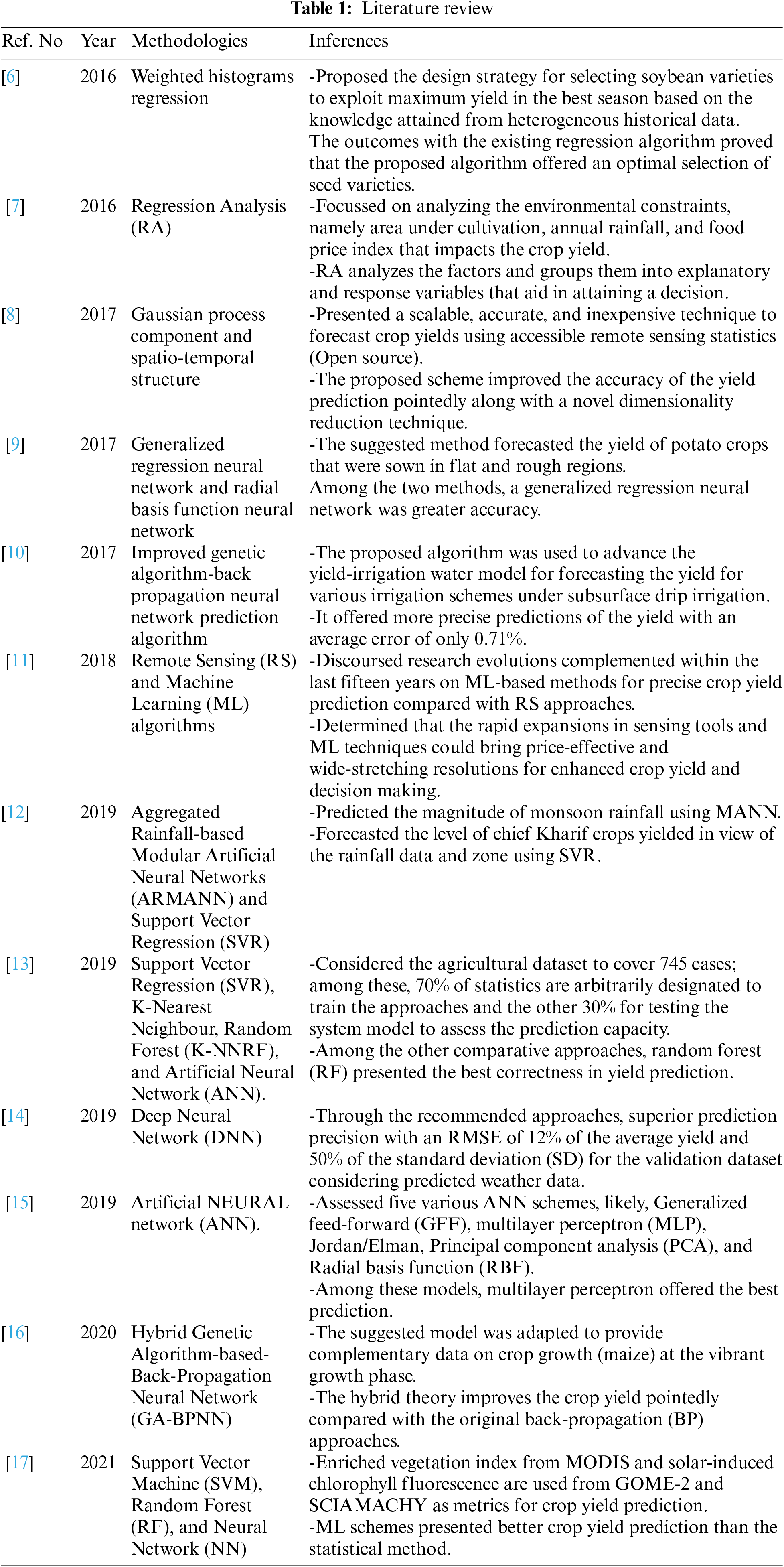
Formerly, researchers estimate the crop yield using statistical approaches, including the multivariate linear regression (MLR) technique. However, the prediction accuracy was not up to the expectation. Currently, machine learning (ML) approaches are growing as a powerful descriptive and predictive tool in handling complex research problems. Crop yield prediction is one of the challenging problems in precision agriculture, and many models have been proposed in the literature and validated so far. Crop yield prediction at its early stage is a difficult task. The Agricultural yield primarily depends on weather conditions (rain, temperature, etc.) and pesticides. Accurate information about crop yield history is essential for making decisions related to agricultural risk management and future predictions. Many studies have used statistical models such as regression, multivariate regression, and artificial neural networks for crop yield prediction with limited input parameters. The table below illustrates the exiting works relating to crop yield prediction using various methodologies and spectrums (Tab. 1).

Further, Gu et al. [18] proposed a hybrid model using a back-propagation algorithm combined with a genetic algorithm for forecasting the corn yield for diverse irrigation systems and found the average error to be only 0.71%. Also, Kodimalar et al. [19] investigated a pool of machine learning techniques in the big data computing model and recommended SVM and ANN to be the most appropriate ML models for rice yield prediction. Furthermore, Maya Gopal et al. [7] found the Forward Feature Selection algorithm integrated with random forest algorithm to efficiently select the appropriate input parameters for accurate crop yield prediction. Moreover, Mohsen et al. [20] designed a few more ensemble models considering the complete and partial in-season weather knowledge with the blocked sequential procedure and achieved 9.5% RRMSE by the optimized weighted ensemble and the average ensemble models. Cai et al. [21] compared the regression-based methods with machine learning methods in their performance in Wheat yield prediction in Australia and concluded machine learning methods to have higher performance with R² as 0.75 at two months advance time before the wheat maturity time. Eventually, Ansarifar et al. [22] attempted to select the most tightfitting environmental and management parameters and to find the extent of interaction within them about the crop yield using the interaction regression model and achieved an RRMSE of less than 8%.

The rest of this paper is organized as follows. In Section 2, the dataset and site descriptions are provided along with each input parameter and the target value. In Section 3, the theory behind the statistical model and the machine learning models are explained. In Section 4, the performance of each model is discussed in detail, and Section 5 concludes the paper.

2  Data Collection and Site Descriptions

Paddy is the main crop in Tamil Nadu produced in massive quantity in almost all the districts of this state, and so the rice production data were considered for this research. The data utilized in this paper includes 470 samples collected from the 28 districts of Tamil Nadu (Fig. 1) during the Kharif season (June–Sep) for a period of 18 years from 1998 to 2015 over a field size of 1 hectare. Since Kharif is the primary season for rice production in Tamil Nadu, all the other parameter values are limited to this season only.

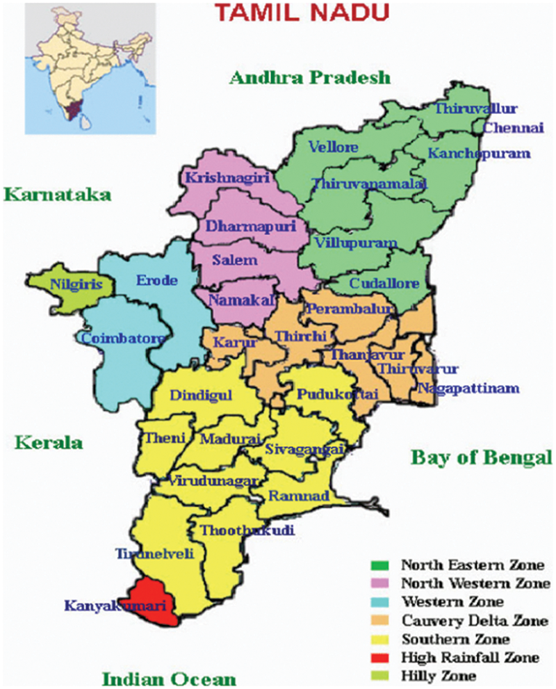
Figure 1: Cropping zone for rice in different districts of Tamil Nadu

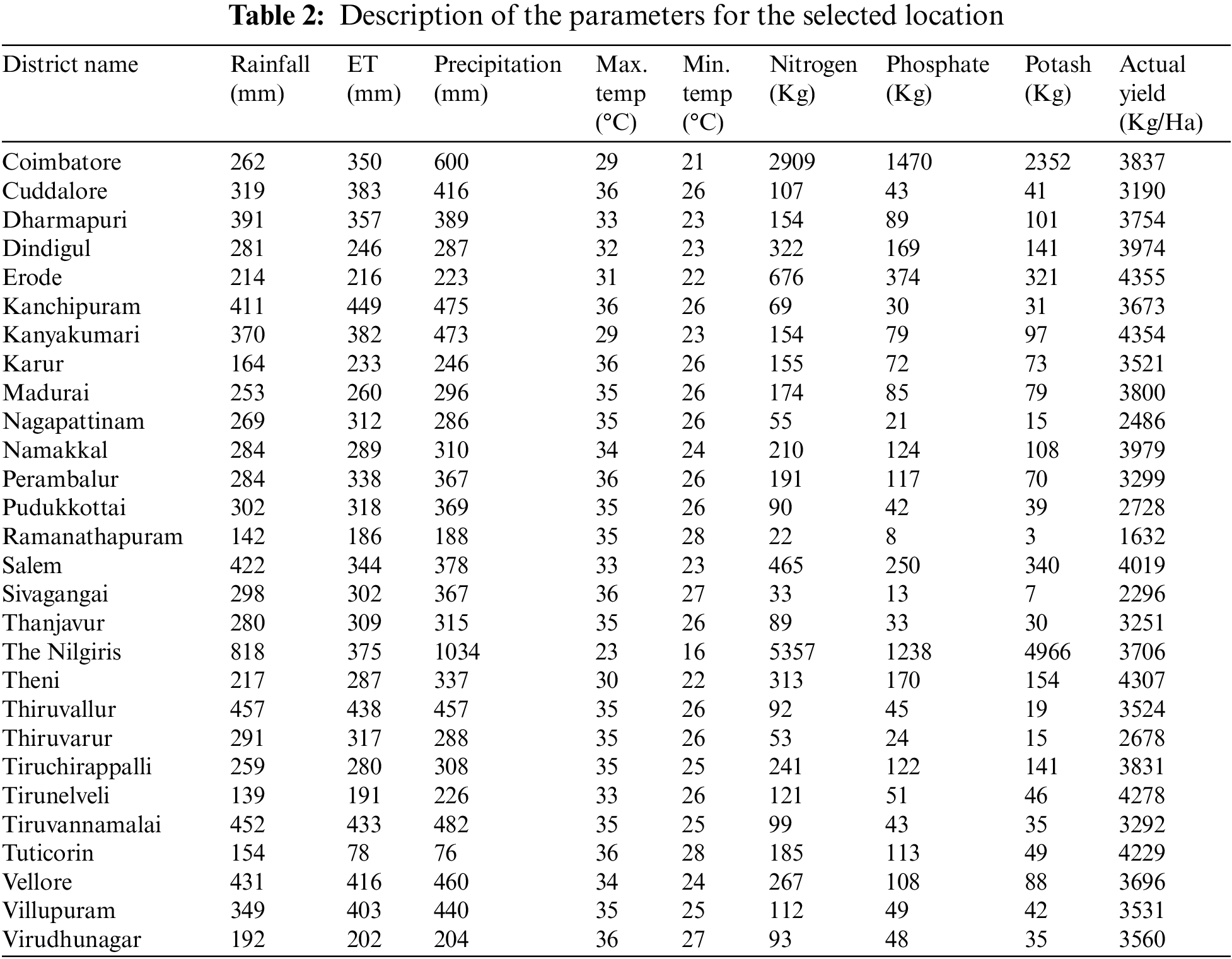
Eight input parameters were considered for each of these 28 districts in the dataset viz. Rainfall (mm), Evapotranspiration (mm), Precipitation (mm), Maximum temperature (°C), Minimum temperature (°C), Fertilizers (Nitrogen, Phosphorus, Potash) (Kg) as mentioned in Tab. 2. The crop yield in kg/ha is taken as the target variable. The mean values of all the parameters are also described. The data were collected from the agricultural department of Tamilnadu [23], Regional Meteorological Centre–Chennai [24], Tata-Cornell Institute for Agriculture and Nutrition (TCI) [25], and the statistical department of Tamilnadu [26].

3  Methodologies

3.1 Statistical Analysis

To estimate the yield, a multiple linear regression (MLR) was applied. MLR is a well-knownmethod used to derive the relationship between a dependent variable and one or more independent variables. The following equation describes the MLR [27]

y=b0+b1x1+⋯bpxp+e(1)

where y is the predicted variable, xi(i = 1, 2, …, P) are the predictors, b0 is called intercept (coordinate at origin), bi(i = 1, 2, …, P) is the coefficient on the ith predictor, and e is the error associated with the predictor.

3.2 Machine Learning Techniques

3.2.1 Back Propagation Neural Network (BPNN)

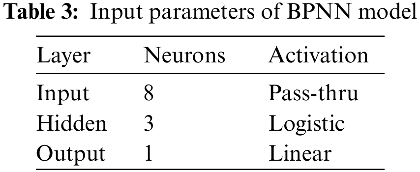
The neural network is a circuit of neurons, and the Backpropagation neural network comes under a supervised learning algorithm for training multilayer perceptron. In this model, eight neurons are in the input layer for eight input parameters. Further, random weights are initiated, and a bias value is added. At the hidden layer, three neurons are passed through the logistic regression activation function along with their weights and then reach the single neuron output layer. The BPNN tries to minimize the error function in weight space using the delta rule or gradient descent. The weights that minimize the error function to a global optimum are considered a solution to the learning problem [28]. The architecture of the BPNN model and the input parameters are given in Fig. 2 and Tab. 3, respectively. The neurons execute summation of all weighted inputs and determine the sum for activation function (f):

Hn=f(wIm,nIm)(2)

Ol=f(wHn,lHn)(3)

where Hn denotes a hidden layer (subscript n represent a neuron); Ol terms a neuron output; Im is the input; wIm,n and wHn,l are the weights of synaptic.

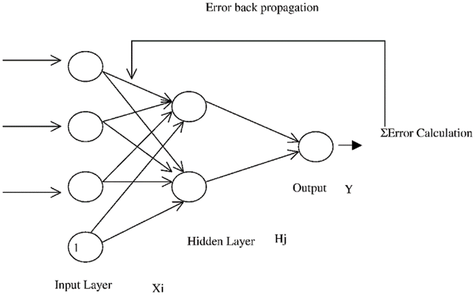
Figure 2: Architecture of BPNN

Then the hyperbolic tangential sigmoid function can be derived as follows:

f(x)=2(1+e−2x)−1(4)

The linear transfer function can be expressed using the below equation that can be applied to the output layer.

f(x)=x(5)

The normalized equation needs to apply to force the data to be maintained between the defined ranges.

YN=(ymax−ymin)×(xi−xminxmax−xmin)+ymin(6)

where YN represent normalized value; xmin and xmax are the minimum and maximum range of data; ymin and ymax are −1 and 1, respectively.

3.2.2 Support Vector Machine (SVM)

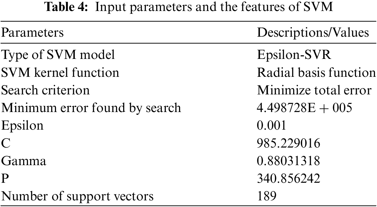
Using Support Vector Machine aims to identify a hyperplane in an N-dimensional space to distinguish the data points. In Support Vector Regression, the margins are chosen to cover maximum data points leaving a few moments considered as slack variables. SVR is a very efficient algorithm because it is determined by the support vectors that cover the margin boundaries. Moreover, the SVR has a very efficient option to incorporate nonlinearity using the kernel trick. In our model, we used Radial basis function as the kernel function. The input parameters used for the model are derived in Tab. 4. The data samples are fitted concerning function fitting problems of the SVM;{xi,yi},(i=1,2,…,n),xi∈Rnyi∈R with function f(x)=w×(x+b). According to SVM theory, the fitting problem can be derived as follows [28]:

f(x)=w×(x+b)=∑i=1k⁡(ai−ai∗)K(xxi)+b(7)

The ranges of ai,ai∗,b are obtained through second optimization problems. Generally, a small portion of ai,ai∗ should not be zero and named as a support vector.

Max:

w(a,ai∗)=−12∑i,j=1k⁡(ai−ai∗)(aj−aj∗)K(xixj)+∑i=1k⁡yi(ai−ai∗)−∈∑i=1k⁡(ai+ai∗)(8)

s.t.{∑i,j=1k⁡(ai−ai∗)=00≤ai,ai∗≤C,(i=1,2…,k}(9)

where, C is a constant that represent a penalty factor and indicates the penalty degree for excessive error; (xixj) is a kernel function. The following are the different types of Kernel functions at present:

1.    Linear kernel:

(x, y)=x\ast y(10)

2.    Polynomial kernel:

K (x, y)=[(x\ast y)+1](d=1, 2 …)(11)

3.    Radial primary kernel function:

K (x, y)=exp[− ‖x−y ‖2σ2]2(12)

4.    Two layers neural kernel:

K (x, y)=tanh [a (x\ast y)−δ]2(13)

3.2.3 General Regression Neural Network (GRNN)

General Regression neural network is an improved technique of RBF neural network which is more suitable for regression problems, particularly for dynamic systems like yield prediction. The architecture of the model is illustrated in Fig. 3. In this model, every data will represent a mean to a radial basis neuron. It has four layers: The input layer, hidden layer, summation layer, and the decision layer. GRNN is mathematically expressed as follows:

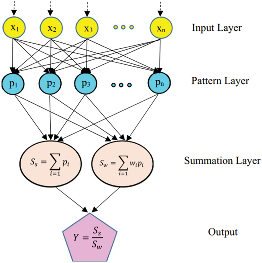
Figure 3: Architecture of GRNN

This summation layer feeds the numerator and denominator parts to the output layer. The regression of y on X can be derived as follows:

E⟨y|X⟩=∫−∞∞⁡yf(X,y)dy∫−∞∞⁡f(X,y)dy(14)

The probability estimator f^(X,Y) can be derived using the below equation based on the values of XIandYi of the random variables x and y, respectively.

f^(X,Y)=12π(p+1)/2σ(p+1)1n×∑i=1n⁡exp[−(X−Xi)T(X−Xi)2σ2]exp[−(Y−Yi)22σ2](15)

where n represents the number of sample observations; p denotes a vector variable x; σ terms the width of each sample. Then the scalar function D2 can be derived as follows:

Di2=(X−Xi)T(X−Xi)(16)

The output layer consists of one neuron, which determines the output that yields the predicted output Y(x) to an unknown input vector x using the below formula:

Y^(X)=∑Yi⁡e−(Di22σ2)∑e−(Di22σ2)(17)

Euclidian distance from Xi to X and e−(di22σ2) is an activation function.

The activation function is the weight of the input data. At this point, the unknown spread parameter is constant (σ), and it can be adjusted by the training process to an optimum range where the error should be minimized. The training procedure is to determine the optimum of σ, and it varies between 0.0001 and 1. Therefore, the best practice is to minimize the MSE, and all normalized 100 data sets are divided into training and testing datasets as per the thumb rule. The network's training is carried out on 70% of data sets, and the remaining data sets were used to test and evaluate the network using as considered for the previous model.

4  Results and Discussions

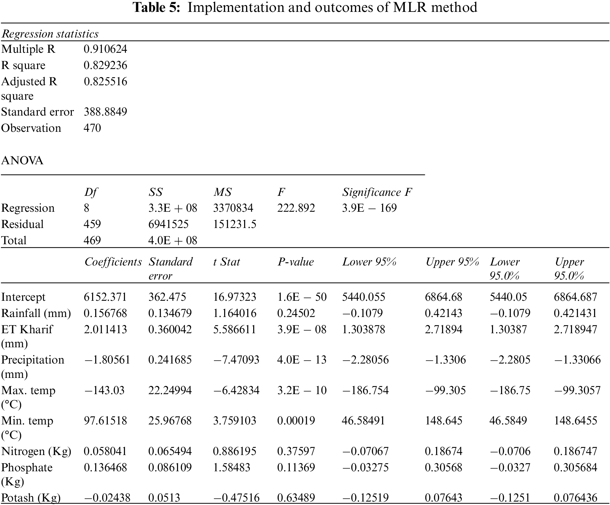
4.1 Multi Linear Regression (MLR)

MLR model was developed based on the input-independent variables like Rice area, Rice production, rainfall, ET, Precipitation, temperature and fertilizers, and the output-dependent variable, the crop yield. The following equation represented the estimated output based on MLR:

yield=6152.37+0.157∗Rainfall+2.011∗ET−1.8∗Precipitation−143.03∗Maximum Temperature+97.62∗Minimum Temperature+0.058∗Nitrogen+0.136∗Phosphate−0.024∗Potash

The paddy yield prediction of the MLR model is plotted between actual and predicted values in terms of kg/Ha (Fig. 4). It is noted that there is an inaccurate characteristic found between the yields. Further, the regression statistics illustrated in Tab. 5 show acceptable ranges i.e., multiple R, R2, and adjusted R and standard deviation are 0.910624, 0.8292236, 0.825516 388.8849, respectively.

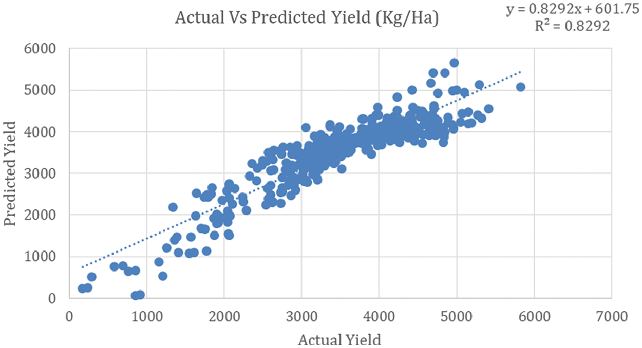
Figure 4: MLR model

Considering the non-significance values of observed results from the MLR model, it is essential to demonstrate the machine learning models to precisely predict crop yield. Therefore, the following sections attempt various machine learning approaches for crop yield prediction.

4.2 Machine Learning Models

Further, for better visualization, different machine learning models such as back-propagation neural network (BPNN), Support Vector Machine (SVM), and General Regression Neural Network (GRNN) is demonstrated in a virtual platform that generates a graph between actual and predicted yield. The simulated plot for each model is given in Fig. 5.

From the observed images, it is perceived that the best fit of the three models shows better accuracy between actual and predicted yield. Among the three models, such as BPNN, SVM, and GRNN, the prediction curve best fits the actual yield precisely in the GRNN model. It can be ensured using the distributed dots in the plotted images.

Also, to make the potential yield more practical, conciseness, and readable, the time-series analysis model experiments for all the considered machine learning approaches. These models of representation clearly distinguish the predicted yield and the actual yield and show the validated samples separate from the training samples. The simulated results of each model are illustrated in Fig. 6.

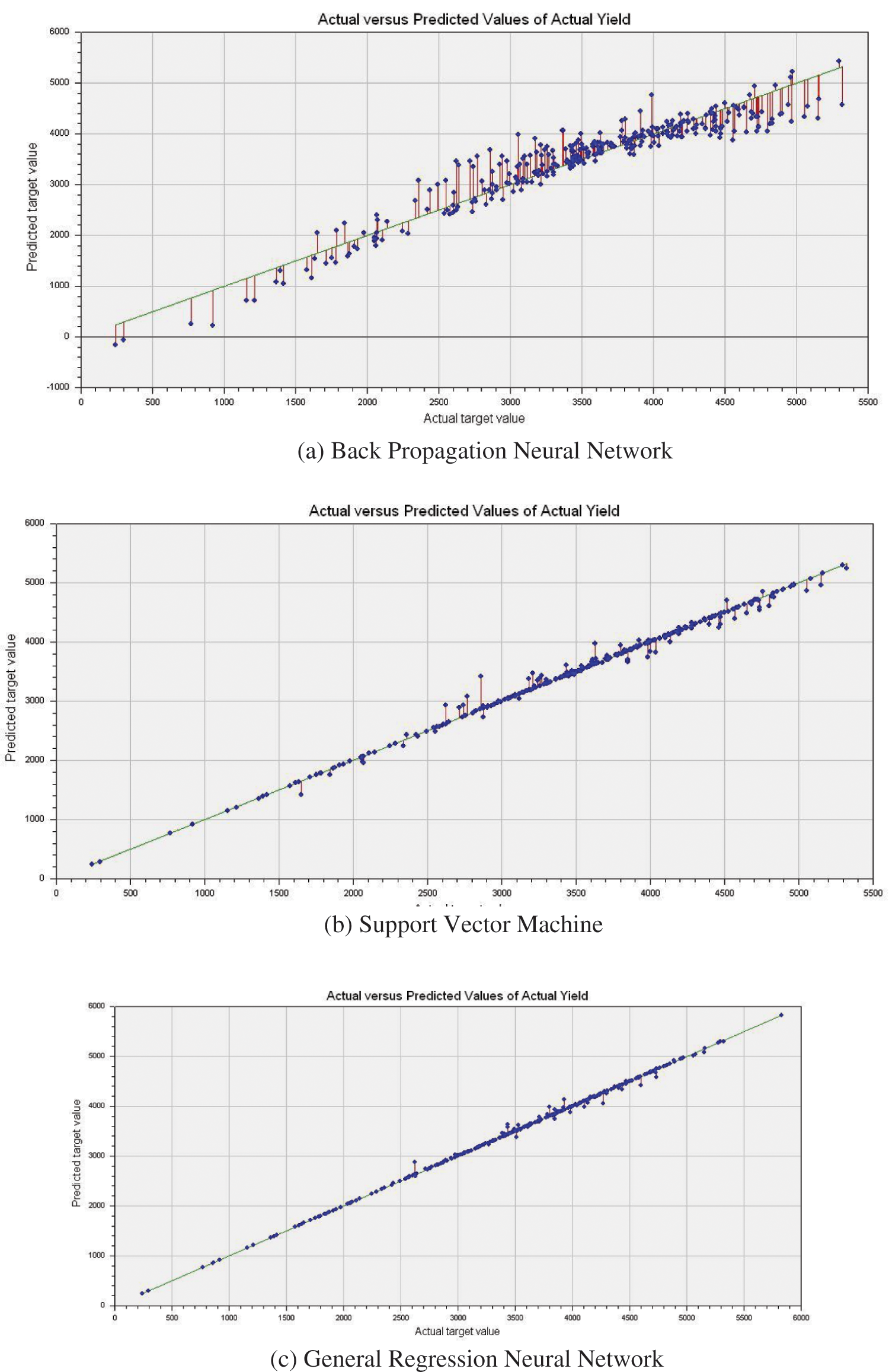
Figure 5: Actual vs. predicted crop yield

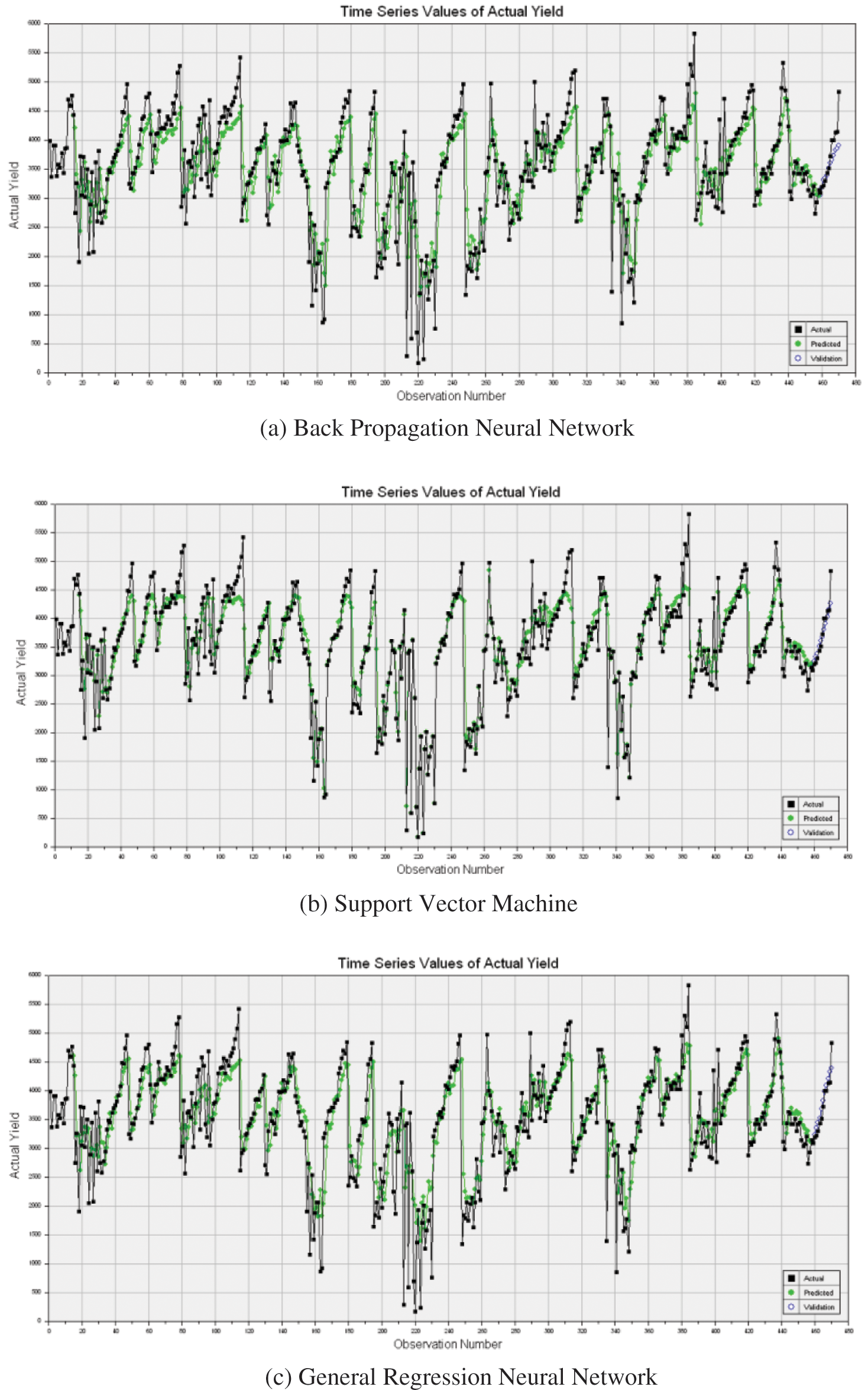
Figure 6: Time series model (actual vs. predicted values)

As shown in the above figures, the time-series results show the prediction accuracy between actual and predicted values. It is observed that all the models show good accuracy; however, a GRNN model illustrates a more precise prediction among other approaches. It can be further ensured using evaluation metrics as described in the following section.

4.3 Evaluation Metrics for Machine Learning Models

The effectiveness of the machine learning models was gauged by using the following seven evaluation metrics. The values obtained by each model in these metrics are shown in Tab. 6.

✓   The proportion of variance explained by model (R2): In a regression problem, R2 denotes the amount of deviation of the dependent variables explained by the independent variable.

R2=1−(unexplainedvariance/totalvariance)(18)

It is considered that the R2 value of MLR method as a benchmark, i.e., 0.82 and analyzed the same with the ML models and found the R2 as 0.89, 0.93, and 0.97 for BPNN, SVM, and GRNN models, respectively. GRNN has the potential to explain 97% of variance from the input parameters towards the yield, thereby offering higher prediction accuracy.

✓   Coefficient of variation (CV): It is a valuable tool to compare the results of two models and say which has more variance in relevance to its mean.

Coefficientofvariation=(StandardDeviation/Mean)∗100(19)

In this work, CVs are observed as 0.08, 0.07, and 0.05 for BPNN, SVM, and GRNN models, respectively. BPNN shows more variance among these ranges, and GRNN has the least variance.

✓   Normalized mean square error (NMSE): This metric is considered a practical test for model performance, overviewing the entire data set of samples unbiased towards over or under prediction.

NMSE=‖yi−y¯i‖22‖y¯i‖22(20)

The NMSE values of BPNN, SVM, and GRNN are found to be 0.11, 0.07, and 0.03, respectively. It is noticed that the error rate is very minimum for the GRNN model.

✓   Maximum Error of Estimation: It points out the accuracy of the prediction, and it is defined as 50% of the width of a confidence interval. It is also called the margin of error. SVM has the least error estimate of 560.65 as it takes only the margin values (support vectors) under consideration; whereas, GRNN has a maximum error of 1031.02 because of the Euclidean distance of every sample is considered for each estimate.

✓   Root Mean Squared Error: It is the measure of how far the data points are spread around the best fit line. Statistically, it is the standard deviation of the residuals.

RMSE=∑i=0n⁡|Ai−Pi|2n(21)

The RMSE value for BPNN, SVM, and GRNN is evaluated to be 296.07, 234.65, and 161.47, respectively. This metric shows that the predictions of the GRNN model are very close to the best fit line with an RMSE of 161.47 taken from 470 fields spread over the state of Tamilnadu.

✓   Mean Absolute Error: Absolute error measures the magnitude of difference between the actual yield and predicted yield. MAE is the mean of the absolute error.

MAE=1N∑i=1N⁡|Yi−Y⇀i|(22)

From the considered models, MAEs are found to be 215.34, 132.82, and 82.74 for BPNN, SVM, and GRNN, respectively. The observed MAE of the GRNN model (82.74) represents a minimum error for the entire group of measured samples compared with other models.

✓   Mean Absolute Percentage Error (MAPE): MAPE is calculated by applying the mean function on the MAE values.

MAPE=1N∑i=1N⁡|Yi−Y⇀iYi|×100(23)

When MAPE value gets lower and further lower, it represents an arrival of a better fit line. Among the models, GRNN has a very low MAPE of 3.11, indicating a better fit compared with other models.

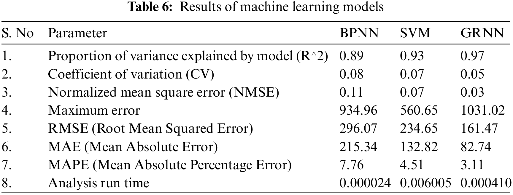
From the obtained results of the machine learning models through the seven metrics, the following observations were noted: BPNN takes comparatively less time for analysis, but the deviation of the prediction from actual yield was more, and hence it is less efficient. The SVM has relatively more accuracy than BPNN, but it takes more time to train and validate the model. The GRNN analyses have the highest performance in predicting the crop yield in a diverse environment with R2 of 0.97. Further, the run time analysis is carried out for all models; it is the time taken for the model to arrive at a better fit line. It is observed that BPNN has a less time of 24 μs, whereas SVM and GRNN take 60 and 4 ms, respectively.

5  Conclusions

Crop yield prediction plays a significant role in the agricultural sector that can be performed using statistical and machine learning algorithms. In this work, statistical models namely MLR and machine learning models such as BPNN, SVM, and GRNN models, are demonstrated for wide-area spectrum considering the Indian state of Tamilnadu. Seven different evaluation metrics are derived from warranting the reliability of the observed results. Based on the attained results, the following conclusions are made:

✓   Compared with the statistical model (MLR), ML models offered better accuracy between actual and predicted values, and the same was verified using time series analysis.

✓   GRNN model had a more significant potential to explain 97% of variance from the input parameters towards the crop yield; offered higher prediction accuracy.

✓   BPNN showed more variance (CV), i.e., 0.08, and GRNN has the smallest variance scale of about 0.05.

✓   NMSE and RMSE were found to be least for the GRNN model, i.e., 0.03 and 161.47, respectively: most minor scale among other ML approaches.

✓   MAE and MAPE were observed best range for the GRNN model compared with other models, i.e., 82.74 and 3.11, respectively.

✓   The only limitation of the GRNN model was the run time. BPNN took just 24 μs, whereas GRNN took about and 4 ms.

Consolidating all the inferences, it can be concluded that the GRNN model is more suitable for crop yield prediction for a broad spectrum owing to its superior prediction accuracy.

Funding Statement: This study was supported by Suranaree University of Technology, Thailand.

Conflicts of Interest: The authors declare that they have no conflicts of interest to report regarding the present study.

References

 1.  India economic survey 2018, “Farmers gain as agriculture mechanization speeds up, but more R&D needed,” The Financial Express, 29 January 2018. [Google Scholar]

 2.  A. A. Khan, C. Wechtaisong, F. A. Khan and N. Ahmad, “A cost-efficient environment monitoring robotic vehicle for smart industries,” CMC-Computers, Materials & Continua, vol. 12, pp. 473--487, 2022. [Google Scholar]

 3.  T. V. Klompenburga, A. Kassahuna and C. Catal, “Crop yield prediction using machine learning: A systematic literature review,” Computers and Electronics in Agriculture, vol. 177, pp. 105709, 2020. [Google Scholar]

 4.  A. A. Khan, P. Uthansakul, P. Duangmanee and M. Uthansakul, “Energy efficient design of massive MIMO by considering the effects of nonlinear amplifiers,” Energies, vol. 11, pp. 1045, 2018. [Google Scholar]

 5.  P. Uthansakul and A. A. Khan, “Enhancing the energy efficiency of mm wave massive MIMO by modifying the RF circuit configuration,” Energies, vol. 12, pp. 4356, 2019. [Google Scholar]

 6.  V. Sellam and E. Poovammal, “Prediction of crop yield using regression analysis,” Indian Journal of Science and Technology,” vol. 9, no. 38, pp. 1–5, 2016. [Google Scholar]

 7.  P. S. MayaGopal and R. Bhargavi, “Performance evaluation of best feature subsets for crop yield prediction using machine learning algorithms, “Applied Artificial Intelligence, vol. 33, no. 7, pp. 621–642, 2019. [Google Scholar]

 8.  O. Marko, S. Brdar, M. Panic, P. Lugonja and V. Crnojevic, “Soybean varieties portfolio optimisation based on yield prediction,”Computers and Electronics in Agriculture, vol. 127, pp. 467–474, 2016. [Google Scholar]

 9.  A. Chlingaryan, S. Sukkarieh and B. Whelan, “Machine learning approaches for crop yield prediction and nitrogen status estimation in precision agriculture: A review,” Computers and Electronics in Agriculture, vol. 151, pp. 61–69, 2018. [Google Scholar]

10. P. Uthansakul and A. A. Khan, “On the energy efficiency of millimeter wave massive MIMO based on hybrid architecture,” Energies, vol. 12, pp. 2227, 2019. [Google Scholar]

11. A. Pandey and A. Mishra, “Application of artificial neural networks in yield prediction of potato crop,” Russian Agricultural Sciences, vol. 43, no. 3, pp. 266–272, 2017. [Google Scholar]

12. L. Wang, P. Wang, S. Liang, Y. Zhu, J. Khan et al., “Monitoring maize growth on the north China plain using a hybrid genetic algorithm-based back-propagation neural network model,” Computers and Electronics in Agriculture, vol. 170, pp. 105238, 2020. [Google Scholar]

13. J. You, X. Li, M. Low, D. Lobell and S. Ermon, “Deep gaussian process for crop yield prediction based on remote sensing data,” in Proc. of the Thirty-First AAAI Conf. on Artificial Intelligence (AAAI-17), California, USA, pp. 1–5, 2017. [Google Scholar]

14. J. Gu, G. Yin, P. Huang, J. Guo and L. Chen, “An improved back propagation neural network prediction model for subsurface drip irrigation system,” Computers & Electrical Engineering, vol. 60, pp. 58–65, 2017. [Google Scholar]

15. M. Abdipour, M. Younessi-Hmazekhanlu, S. H. R. Ramazani and A. H. Omidi, “Artificial neural networks and multiple linear regression as potential methods for modeling seed yield of safflower (Carthamustinctorius L.),” Industrial Crops and Products, vol. 127, pp. 185–194, 2019. [Google Scholar]

16. I. Esfandiarpour-Boroujeni, E. Karimi, H. Shirani, H. M. Esmaeilizadeh and Z. Mosleh, “Yield prediction of apricot using a hybrid particle swarm optimization-imperialist competitive algorithm-support vector regression (PSO-ICA-SVR) method,” ScientiaHorticulturae, vol. 257, pp. 108756, 2019. [Google Scholar]

17. Y. Cai, K. Guan, D. Lobell, A. B. Potgieter, S. Wang et al., “Integrating satellite and climate data to predict wheat yield in Australia using machine learning approaches,” Agricultural and Forest Meteorology, vol. 274, pp. 144–159, 2019. [Google Scholar]

18. J. Gu, G. Yin, P. Huang, J. Guo and L. Chen, “An improved back propagation neural network prediction model for subsurface drip irrigation system,” Computers and Electrical Engineering, vol. 60, pp. 58–65, 2017. [Google Scholar]

19. P. Kodimalar and S. Chellammal, “An approach for prediction of crop yield using machine learning and big data techniques,” International Journal of Computer Engineering and Technology (IJCET), vol. 10, no. 3, pp. 110–118, 2019. [Google Scholar]

20. S. Mohsen, G. Hu and V. Sotirios, “Forecasting corn yield with machine learning ensembles,” Frontiers in Plant Science, vol. 11, pp. 3427, 2020. [Google Scholar]

21. Y. Cai, “Integrating satellite and climate data to predict wheat yield in Australia using machine learning approaches,” Agricultural and Forest Meteorology, vol. 274, pp. 144–159, 2019. [Google Scholar]

22. J. Ansarifar, L. Wang and S. Archontoulis, “An interaction regression model for crop yield prediction,” Nature portfolio, Scientific Reports, vol. 11, pp. 17754, 2021. [Google Scholar]

23. A. A. Khan and F. A. Khan, “A cost-efficient radiation monitoring system for nuclear sites: Designing and implementation,” Intelligent Automation & Soft Computing, vol. 32, pp. 1357--1367, 2022. [Google Scholar]

24. A. A. Khan, P. Uthansakul and M. Uthansakul, “Energy efficient design of massive MIMO by incorporating with mutual coupling,” International Journal on Communications Antenna and Propagation (IRECAP), vol. 7, no. 3, pp. 198--207, 2017. [Google Scholar]

25. A. Hassan, R. M. Asif, A. U. Rehman, Z. Nishtar, M. K. A. Kaabar et al., “Design and development of an irrigation mobile robot,” IAES International Journal of Robotics and Automation (IJRA), vol. 10, no. 2, pp. 75--90, 2021. [Google Scholar]

26. J. Arshad, M. Aziz, A. Asma, A. Huqail, M. H. Zaman et al., “Implementation of a LoRaWAN based smart agriculture decision support system for optimum crop yield,” Sustainability, vol. 14, no. 2, pp. 827, 2022. [Google Scholar]

27. S. Mishra, D. Mishra and G. H. Santra, “Applications of machine learning techniques in agricultural crop production: A review paper,” Indian Journal of Science and Technology, vol. 9, no. 38, pp. 56756, 2016. [Google Scholar]

28. V. Joshua, S. M. Priyadharson and R. Kannadasan, “Exploration of machine learning approaches for paddy yield prediction in eastern part of Tamilnadu,” Agronomy, vol. 11, pp. 2068, 2021. [Google Scholar]

This work is licensed under a Creative Commons Attribution 4.0 International License, which permits unrestricted use, distribution, and reproduction in any medium, provided the original work is properly cited.