Computers, Materials & Continua DOI:10.32604/cmc.2022.027197
Article

A Novel Method for Precipitation Nowcasting Based on ST-LSTM

Wei Fang1,2,*, Liang Shen1, Victor S. Sheng3 and Qiongying Xue1

1School of Computer & Software, Engineering Research Center of Digital Forensics, Ministry of Education, Nanjing University of Information Science & Technology, Nanjing, 210044, China
2State Key Laboratory of Severe Weather, Chinese Academy of Meteorological Sciences, Beijing, 100081, China
3Department of Computer, Texas Tech University, Lubbock, TX, 79409, USA
*Corresponding Author: Wei Fang. Email: Fangwei@nuist.edu.cn
Received: 12 January 2022; Accepted: 04 March 2022

Abstract: Precipitation nowcasting is of great significance for severe convective weather warnings. Radar echo extrapolation is a commonly used precipitation nowcasting method. However, the traditional radar echo extrapolation methods are encountered with the dilemma of low prediction accuracy and extrapolation ambiguity. The reason is that those methods cannot retain important long-term information and fail to capture short-term motion information from the long-range data stream. In order to solve the above problems, we select the spatiotemporal long short-term memory (ST-LSTM) as the recurrent unit of the model and integrate the 3D convolution operation in it to strengthen the model's ability to capture short-term motion information which plays a vital role in the prediction of radar echo motion trends. For the purpose of enhancing the model's ability to retain long-term important information, we also introduce the channel attention mechanism to achieve this goal. In the experiment, the training and testing datasets are constructed using radar data of Shanghai, we compare our model with three benchmark models under the reflectance thresholds of 15 and 25. Experimental results demonstrate that the proposed model outperforms the three benchmark models in radar echo extrapolation task, which obtains a higher accuracy rate and improves the clarity of the extrapolated image.

Keywords: Precipitation nowcasting; radar echo extrapolation; ST-LSTM; attention mechanism

1  Introduction

Precipitation nowcasting refers to short-term weather forecasts within 2 h, which focuses on small and medium-scale meteorological systems, such as severe convective weather. This task aims to give a precise and timely prediction of rainfall intensity in a local region over a relatively short period [1]. Compared with long-term precipitation forecasts, it has higher requirements in terms of accuracy and timeliness. Accurate prediction of short-term precipitation can assist people in assessing road water accumulation, guiding traffic, and improving the accuracy of early warning of heavy precipitation in cities, which is of great significance for disaster prevention and mitigation.

Radar echo extrapolation is an important method for precipitation nowcasting. Traditional morphological-based radar echo extrapolation techniques mainly include the cross-correlation method [2,3] and the single centroid method [4,5]. The cross-correlation method selects two consecutive times of spatial optimization correlation coefficients to establish a fitting relationship but it has low data utilization which brings the problem of low prediction accuracy. The centroid tracking method can achieve better results in stable precipitation forecasting [6]. But for the echoes which evolve quickly, this method cannot meet the conservation conditions and the forecasting effect will rapidly decrease with time. The optical flow method [7] is a widely used method for extrapolating radar echoes. This method calculates the optical flow field from a continuous image sequence, and uses the changes in the time domain of pixels in the image sequence and the correlation between adjacent frames to establish the correspondence between the previous frame, and then calculate the motion information of the object between adjacent frames, the optical flow method can capture the motion and change information of the radar echo, but it does not make full use of the echo image information over a longer period of time.

In recent years, Deep learning methods is a hot research topic. Shi et al. [8] proposed a convolutional long short-term memory (ConvLSTM) neural network structure based on LSTM, which achieves a higher prediction accuracy than the optical flow method. Since then, many improved variant structures have been developed based on ConvLSTM. For example, Shi [9] introduced the idea of optical flow trajectory and proposed Trajectory GRU (TrajGRU), which can learn the position change information of echo and further improve the accuracy of prediction. Villegas et al. [10] combined the encoder-decoder structure and ConvLSTM to establish a motion and content decomposition model. This model simplifies the prediction task, effectively handles the complex evolution of pixels in the video, and can independently capture the spatial structure of the image and the corresponding time dynamics. Wang introduced spatial memory unit (ST-LSTM) in ConvLSTM and proposed PredRNN [11] to enhance the ability to capture short-term dynamic changes by using a larger convolutional neural receptive field. Wang et al. [12] proposed the Memory in Memory model to learn high-level nonlinear spatiotemporal dynamic information. Lin et al. [13] proposed a self-attention mechanism ConvLSTM, which effectively captures long-term spatial dependencies. Xu et al. [14] combined the generation ability of GAN with the predictive ability of the LSTM network and proposed a Generative Adversarial Network Long Short-term Memory (GAN-LSTM) model for spatiotemporal sequence prediction. Compared with traditional methods, the radar echo extrapolation methods based on deep learning have the advantages of high data utilization efficiency, accurate prediction accuracy, and great optimization potential.

Although the radar echo extrapolation methods based on deep learning perform well compared with the traditional methods, those methods still have some problems. The above-mentioned methods lack the ability to capture motion information between adjacent data and cannot fully extract important information from long-term information. Therefore, it remains challenging and requires principled approaches to design an effective spatiotemporal network. To this end, we propose a novel model which integrates 3D convolutions to capture motion information between adjacent time steps. Our experimental results show that 3D convolution is effective for modeling local representations in a consecutive manner. On the other hand, for long-term important feature information, we exploit an attention mechanism based on channels to extract important feature information from the long-term information stream. Experiments show that our model effectively improves the accuracy of radar echo extrapolation and solves the problem of ambiguity in extrapolation.

2  Related Work

2.1 Spatiotemporal Sequence Forecasting

Radar echo extrapolation is essentially a spatiotemporal sequence forecasting problem that has been widely used in precipitation nowcasting [15,16], traffic flow prediction [17–20], and other fields [21] and led to a variety of architectures in deep learning. The current spatiotemporal sequence prediction method has undergone the evolution from the simple LSTM method to the joint convolutional network [8] to the structurally changed PredRNN [11], Memory In Memory [12] and EIDETIC 3D LSTM [22]. Those models inevitably suffer from image blurring and low resolution, which greatly limits the availability of the predictions. Other techniques in deep learning, such as attention mechanism, transfer learning, graph neural network, etc., have also achieved good results in spatiotemporal sequence prediction problems. Wang et al. [23] proposed a transfer learning model, which solves the problem of data imbalance in some regions. Song et al. [24] proposed a framework based on graph convolutional neural network, STSGCN, and solve the problem that the graph relationship between data flows changes over time. The above models have achieved good results in the problem of spatiotemporal sequence prediction, but they lack the ability to learn dynamic information between adjacent images which brings the problem of inaccurate prediction of the overall motion trend with the accumulation of errors.

When forecasting spatiotemporal sequence, it is necessary to consider not only the continuity and periodicity in time, but also the spatial correlation between different regions, and these spatial correlations will also change over time. In order to effectively extract temporal dependence and spatial motion information, we chose the ST-LSTM as the model's recurrent unit considering its superior spatiotemporal information extraction capabilities.

2.2 Attention Mechanism in Deep Learning

The attention mechanism is a data processing method in machine learning, which is widely used in various types of machine learning tasks such as natural language processing, image recognition, and speech recognition. The attention mechanism is essentially similar to the human observation mechanism of external things. The Attention mechanism was first applied in natural language processing, mainly to improve the encoding method between texts, and to learn better sequence information after encoding-decoding. In recent years, Hu et al. [25] proposed SENet to learn the correlation between channels which learn feature weights according to the loss function through the network and achieve better results. Wang et al. [26] proposed ECA-NET, which uses a one-dimensional convolutional layer to aggregate cross-channel information to obtain more accurate attention information. Adding an attention mechanism to the model with an appropriate method can effectively improve the feature extraction capability of the model.

Motivated by the convolutional block attention module (CBAM) [27], we integrated the attention mechanism based on channels into our model to improve the ability of the model that learn time dependence and important features from the long-term information.

3  Model

Our model is based on the ST-LSTM unit. Inspired by the 3D CNNs, we use 3D convolution in the recurrent unit to replace the original 2D convolution operation which increases the capture of the motion information of the adjacent time data. To extract important feature information in long-term data, we also add a channel attention mechanism after the last layer of the encoder.

3.1 3D Convolution Integrated into ST-LSTM

In order to use 3D convolution to extract motion information, the original data needs to be processed first. For expanding the input data in the time dimension, we take the multi-frame data in each sliding window as one-time step input which has 3 dimensions in which each dimension indicates the width, height, and time. This data processing process is shown in Fig. 1.

Figure 1: Data processed using a sliding window

The encoder of our model uses ST-LSTM as the recurrent unit. ST-LSTM is proposed by Wang et al. [7]. in PredRNN, which memorizes spatial and temporal characteristics in a unified memory unit, and transmits memory information on both vertical and horizontal levels. After data processing, the internal structure of the ST-LSTM recurrent unit also needs to be modified to be compatible with the input data which has 3 dimensions. According to the characteristic that the input data has three dimensions, we replace the ordinary convolution inside the ST-LSTM with 3D convolution to extract motion information between adjacent data frames. The original ST-LSTM structure is shown in Fig. 2a and the structure of ST-LSTM integrating 3D convolution is illustrated in Fig. 2b.

Figure 2: Comparison of (a) the standard ST-LSTM recurrent unit and (b) the Improved ST-LSTM recurrent unit integrating 3D convolution. ⊙ is the Hadamard product. ⊕ is the matrix sum operation

There are 4 inputs in the ST-LSTM: Xt, the feature maps from encoders or hidden states from the previous layer; Ht−1l, the hidden states from the last time step; Ct−1l, the memory states from last time step, and Mtl−1, the memory states from previous layer. In the recurrent unit. The input gate, input modulation gate, forget gate and output gate no longer depend on the hidden states and cell states from the previous time step at the same layer. Instead, as illustrated in Fig. 2b, they rely on hidden states Ht−1l and cell states Mtl−1 that are updated by the previous layer at current time step. Inside the recurrent unit, We use 3D convolution as a motion perceptron to extract short-term and local motion in the continuous space-time field. The ST-LSTM integrating 3D convolution can be formulated as (1)–(10):

gt=tanh(Wxg∗Xt+Whg∗Ht−1l+bg)(1)

it=σ(Wxi∗Xt+Whi∗Ht−1l+bi)(2)

ft=σ(Wxf∗Xt+Whf∗Ht−1l+bf)(3)

Ctl=ft⊙Ct−1l+it⊙gt(4)

gt′=tanh(Wxg′∗Xt+Whg∗Mtl−1+bg′)(5)

it′=σ(Wxi′∗Xt+Wmi∗Mtl−1+bi′)(6)

ft′=σ(Wxf′∗Xt+Wmf∗Mtl−1+bf′)(7)

Mtl=ft′⊙Mtl−1+it′⊙gt′(8)

ot=σ(Wxo∗Xt+Who∗Ht−1l+Wco∗Ctl+Wmo∗Mtl+bo)(9)

Htl=ot⊙tanh(W1×1)∗[Ctl,Mtl](10)

where σ is the sigmoid function, ∗ is the 3D-Conv operation, ⊙  is the Hadamard product. In general, the propagation of the data stream is divided into two directions: the transmission of time-dependent information in the horizontal direction and the high-level feature information in the vertical direction. The it and ft are input gate and forget gate. The gt is input module gate which contains input information. Ctl is the memory states of current time step. The it^{\prime}, ft^{\prime} and gt^{\prime} are input gate, forget gate and input module which are used to control longitudinal information transmission. The ot and Htl are output gate and the hidden state. Inside the recurrent unit, the left and right parts have two structures similar to LSTM. The left part is used to control the horizontal transmission of time information, and the right part is used to transfer the fused spatiotemporal information. This structure is capable of modeling short-term motion information.

3.2 Attention Mechanism Based on Channels

Radar echo extrapolation is a long-term sequence prediction problem. How to extract important feature information from long-term input data is particularly important. This is the key to improving prediction accuracy and solving the problem of extrapolation ambiguity. To this end, we added the channel attention mechanism into the model to improve the model's ability to extract important features. The overall architecture of the model and the implementation details of the attention module are shown in Fig. 3.

Figure 3: The overall structure of the model and the attention mechanism module

Our work is partially motivated by the convolutional block attention module (CBAM). In our model, the attention mechanism is applied over the output states behind the last layer of the encoder. The formula of the channel attention mechanism is shown in formula (11):

Mc=σ(MLP(AvgPool(F))+MPL(MaxPool(F)))(11)

We first stack the output state of each time step to get a W × H × C feature map F. Then we perform a space global average pooling and maximum pooling respectively to obtain two 1 × 1 × C channel descriptions and send them to a two-layer multilayer perceptron (MLP) network. Finally, the two obtained features are added and passed through a sigmoid activation function to obtain the weight matrix Mc. Each channel of Mc represents a special detector, so it makes sense for channel attention to focus on what information is important for the prediction.

4  Experiments

4.1 Dataset

The radar echo data used in this experiment is the radar mosaic data of Shanghai, which includes three types of scanning products: MDBZ, 2DCR, and MCR. The time interval of each radar data sample is 6 min and the single data presentation form is grid data which indicates the resolution in the latitude and longitude direction. By observing the original data, we found that there are a large number of negative values. Generally speaking, a larger reflectance value indicates a higher probability of precipitation, so negative values can be ignored. Therefore, the negative values in the original data are firstly reset to zero. Another key thing to remember, since the quality of the data will affect the training results, during the construction of the training set, we select the data with the coverage rate of the echo area greater than 1/10 into the dataset. After data preprocessing, our experiment uses 36000 sequences as training, 1000 sequences for validation, and 3000 for the test. Fig. 4 shows the visualization results of the original radar echo sequence data for 5 consecutive frames at three different positions.

Figure 4: Radar echo dataset

4.2 Evaluation Criteria

We evaluate the models by using several commonly used precipitation nowcasting metrics, namely, probability of detection (POD), false alarm rate (FAR), critical success index (CSI), and mean square error (MSE). The CSI, FAR and POD are skill scores similar to precision and recall commonly used by machine learning researchers. Firstly, we convert the prediction and ground truth to a 0/1 matrix by using a selected reflectance threshold which indicates raining or not. Secondly, we calculate the hits (prediction = 1, truth = 1), misses (prediction = 0, truth = 1) and false alarms (prediction = 1, truth = 0). The number of hits, misses, and false alarms are denoted respectively by nsuc, nerr and navo. In the end, we can calculate the value of POD, FAR and CSI by formulas (12)–(14). The MSE metric is defined as the average squared error between the prediction and the ground truth, which is obtained by accumulating all pixel differences. The calculation formula of MSE is shown in formula (15), where yi represents the ground truth and yip represents the predicted value.

POD=nsucnsuc+nerr(12)

FAR=navonsuc+navo(13)

CSI=nsucnsuc+navo+nerr(14)

MSE=∑i=1n⁡(yi−yip)2(15)

SSIM(x,y)=(2μxμy+C1)(2σxy+C2)(μx2+μy2+C1)(σx2+σy2+C2)(16)

For evaluating the visual quality of the images, we measure the similarity of two images using structural similarity index measure (SSIM), which estimates the visual quality of extrapolated images from three aspects: grayscale, contrast, and structure. The calculation formula of SSIM is as formula (16). In the formula, x, y are the pixel values of the two images, μx is the mean of x, μy is the mean of y, σx2 is the variance of x, σy2 is the variance of y, σxy is the covariance of x and y, and C1=(K1L)2,C2=(K1L)2, L is the dynamic range of pixel values, the variation range in the paperis 0–75, K1=0.01,K2=0.01. The SSIM ranges between 0–1, representing the similarity between the generated image and the ground truth.

4.3 Experimental Results and Analysis

In meteorological services, different levels of warnings are often given to different precipitation intensities, with this in mind, the comprehensive performance of the model under different precipitation levels should be used for evaluating the quality of the models. To this end, we select the reflectance threshold of 15 and 25 dBz as the thresholds for binarization according to the climatic characteristics of Shanghai. In the comparison experiment, we considered three benchmark models ConvLSTM [8], PredRNN [11] and TrajGRU [9] to compare with our model under the reflectance threshold of 15 and 25 dBz. All models are trained using the ADAM optimizer with a starting learning rate of 10−3. All experiments are implemented in Pytorch and conducted on NVIDIA 2080TI GPU. We use the POD, FAR, CSI and MSE described above as the metrics for evaluation. Tabs. 1 and 2 show the performance of the evaluated models using a common setting in the literature: generating 10 future frames given the previous 10 frames. Each row in the table records the average value of each model under different metrics.

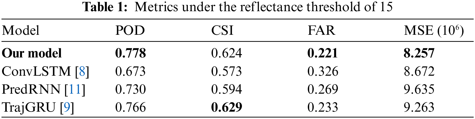
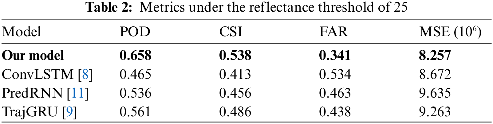
In order to show the experimental results more intuitively, we show the change process of the different metrics through Figs. 5 and 6. In the experiment with the reflectance threshold of 15 dbz, the quantitative results presented in Tab. 1 indicate that our model performs favorably against the three benchmark models. Our model achieves better results than the other three benchmark models in terms of POD, FAR, and MSE. By introducing the idea of optical flow trajectory, TrajGRU can actively learn the position change structure in the cyclic connection, which improves the prediction accuracy of radar echo waveform and achieves the highest CSI value. Although the performance of our model under CSI is parallel to TrajGRU, the overall performance is better than TrajGRU. The results shown in Fig. 5 are consistent with the results in Tab. 1. It can be seen from the figure that our model has a more stable extrapolation effect in the later stage of the extrapolation process. When we select the reflectance threshold as 25 dBz, our model achieved the best performance under all metrics. It can be seen that our model has a better predictive effect for stronger precipitation and our method has a more stable attenuation process over time. Besides, we use the per-frame structural similarity index measure (SSIM) to evaluate the visual quality of images. The comparison results of SSIM are shown in Fig. 7. All four models have high prediction accuracy in the first 12 min, but as the prediction time goes on, the SSIM value of our model is consistently higher than the other models. Our model also achieves better performance under the SSIM metric. In summary, the experiments results suggest that our model is capable of modeling long-range periodical motions effectively.

Figure 5: Comparison results on POD, CSI, FAR (reflectance threshold = 15dBz)

Figure 6: Comparison results on POD, CSI, FAR (reflectance threshold = 25dBz)

Figure 7: SSIM comparison results of the four models

5  Conclusion

In this paper, we proposed a novel model based on ST-LSTM for precipitation nowcasting, which performs well compared with mainstream methods based on deep learning. In Our model, we design the 3D convolution module integrated into the ST-LSTM recurrent unit to enhance the model's ability to capture short-term motion information. In addition, we construct the channel attention module based on time channels to extract important feature information in the long-term sequence to solve the ambiguity problem in the extrapolation. In the experiment, we use the real radar echo image as the test set, and the results show that our model has the best comprehensive performance among different metrics, which effectively improves the accuracy of extrapolation and solves the problem of ambiguity in extrapolation. In the future, we will further optimize the model, improve the model's long-term dependence on the predicted value based on ensuring the existing accuracy, and further solve the problem of ambiguity in extrapolation after 10 frames.

Acknowledgement: This work was supported by the National Natural Science Foundation of China (Grant No. 42075007), and the Open Grants of the State Key Laboratory of Severe Weather (No. 2021LASW-B19).

Funding Statement: The authors received no specific funding for this study.

Conflicts of Interest: The authors declare that they have no conflicts of interest to report regarding the present study.

References

 1.  J. Sun, M. Xue, J. W. Wilson, I. Zawadzki, S. P. Ballard et al., “Use of NWP for nowcasting convective precipitation: Recent progress and challenges,” Bulletin of the American Meteorological Society, vol. 95, no. 3, pp. 409–426, 2014. [Google Scholar]

 2.  G. L. Austin and A. Bellon, “The use of digital weather radar records for short-term precipitation forecasting,” Quarterly Journal of the Royal Meteorological Society, vol. 102, no. 426, pp. 265, 2010. [Google Scholar]

 3.  R. E. Rinehart and E. T. Garvey, “Three-dimensional storm motion detection by conventional weather radar,” Nature, vol. 273, no. 5660, pp. 287–289, 1978. [Google Scholar]

 4.  R. K. Crane, “Automatic cell detection and tracking,” IEEE Transactions on Geoscience Electronics, vol. 17, no. 4, pp. 250–262, 1979. [Google Scholar]

 5.  J. T. Johnson, P. L. MacKeen, A. Witt, E. E. W. Mitchell, G. J. Stumpf et al., “The storm cell identification and tracking algorithm: An enhanced WSR-88D algorithm,” Weather and Forecasting, vol. 13, no. 2, pp. 263–276, 1998. [Google Scholar]

 6.  U. Germann and I. Zawadzki, “Scale-dependence of the predictability of precipitation from continental radar images. part I: Description of the methodology,” Monthly Weather Review, vol. 130, no. 12, pp. 2859–2873, 2002. [Google Scholar]

 7.  N. E. Bowler, C. E. Pierce and A. Seed, “Development of a precipitation nowcasting algorithm based upon optical flow techniques,” Journal of Hydrology, vol. 288, no. 1–2, pp. 74–91, 2004. [Google Scholar]

 8.  X. J. Shi, Z. Chen, H. Wang and D. Yeung, “Convolutional LSTM network: A machine learning approach for precipitation nowcasting,” in Proc. NIPS, Montreal, Canada, pp. 802–810, 2015. [Google Scholar]

 9.  X. J. Shi, Z. Gao, L. Lausen, H. Wang, D. Yeung et al., “Deep learning for precipitation nowcasting: A benchmark and a new model,” in Proc. NIPS, Long Beach, CA, USA, pp. 5617–5627, 2017. [Google Scholar]

10. R. Villegas, J. Yang, S. Hong, X. Lin and H. Lee, “Decomposing motion and content for natural video sequence prediction,” in Proc. ICLR, Toulon, France, 2017. [Google Scholar]

11. Y. B. Wang, M. Long, J. Wang, Z. Gao and P. S. Yu, “PredRNN: Recurrent neural networks for predictive learning using spatiotemporal LSTMs,” in Proc. NIPS, Long Beach, CA, USA, pp. 879–888, 2017. [Google Scholar]

12. Y. Wang, J. Zhang, H. Zhu, M. Long, J. Wang et al., “Memory in memory: A predictive neural network for learning higher-order non-stationarity from spatiotemporal dynamics,” in Proc. CVPR, Long Beach, CA, USA, pp. 9154–9162, 2019. [Google Scholar]

13. Z. Lin, M. Li, Z. Zheng, Y. Cheng and C. Yuan, “Self-attention ConvLSTM for spatiotemporal prediction,” in Proc. AAAI, New York, USA, vol. 34, no. 7, 2020. [Google Scholar]

14. Z. Xu, J. Du, J. Wang, C. Jiang and Y. Ren, “Satellite image prediction relying on GAN and LSTM neural networks,” in Proc. ICC, Shanghai, China, pp. 1–6, 2019. [Google Scholar]

15. W. Fang, F. H. Zhang, V. S. Sheng and Y. W. Ding, “SCENT: A new precipitation nowcasting method based on sparse correspondence and deep neural network,” Neurocomputing, vol. 448, pp. 10–20, 2021. [Google Scholar]

16. W. Fang, L. Pang, W. Yi and V. S. Sheng, “AttEF: Convolutional LSTM encoder-forecaster with attention module for precipitation nowcasting,” Intelligent Automation & Soft Computing, vol. 30, no. 2, pp. 453–466, 2021. [Google Scholar]

17. M. A. Duhayyim, A. A. Albraikan, F. N. Al-Wesabi, H. M. Burbur, M. Alamgeer et al., “Modeling of artificial intelligence based traffic flow prediction with weather conditions,” Computers, Materials & Continua, vol. 71, no. 2, pp. 3953–3968, 2022. [Google Scholar]

18. P. Thamizhazhagan, M. Sujatha, S. Umadevi, K. Priyadarshini, V. S. Parvathy et al., “Ai based traffic flow prediction model for connected and autonomous electric vehicles,” Computers, Materials & Continua, vol. 70, no. 2, pp. 3333–3347, 2022. [Google Scholar]

19. W. Zhang, Y. Yu, Y. Qi, F. Shu and Y. Wang, “Short-term traffic flow prediction based on spatio-temporal analysis and CNN deep learning,” Transportmetrica A: Transport Science, vol. 15, no. 2, pp. 1688–1711, 2019. [Google Scholar]

20. J. Li, H. Li, G. Cui, Y. Kang, Y. Hu et al., “Gacnet: A generative adversarial capsule network for regional epitaxial traffic flow prediction,” Computers, Materials & Continua, vol. 64, no. 2, pp. 925–940, 2020. [Google Scholar]

21. J. Kuo, H. Lin and C. Liu, “Building graduate salary grading prediction model based on deep learning,” Intelligent Automation & Soft Computing, vol. 27, no. 1, pp. 53–68, 2021. [Google Scholar]

22. Y. Wang, L. Jiang, M. H. Yang, L. J. Li, M. Long et al., “Eidetic 3D LSTM: A model for video prediction and beyond,” in Proc. ICLR, New Orleans, LA, USA, 2019. [Google Scholar]

23. L. Wang, X. Geng, X. Ma, F. Liu and Q. Yang, “Cross-city transfer learning for deep spatio-temporal prediction,” in Proc. IJCAI, Macao, China, pp. 1893, 2019. [Google Scholar]

24. C. Song, Y. Lin, S. Guo and H. Wan, “Spatial-temporal synchronous graph convolutional networks: A new framework for spatial-temporal network data forecasting,” in Proc. AAAI, New York, USA, vol. 34, no. 1, pp. 914–921, 2020. [Google Scholar]

25. J. Hu, L. Shen and G. Sun, “Squeeze and excitation networks,” in Proc. CVPR, Salt Lake City, USA, pp. 7132–7141, 2018. [Google Scholar]

26. Q. Wang, B. Wu, P. Zhu, P. Li, W. Zuo et al., “ECA-Net: Efficient channel attention for deep convolutional neural networks,” in Proc. CVPR, Seattle, WA, USA, pp. 11531–11539, 2020. [Google Scholar]

27. S. Woo, J. Park, J. Y. Lee and I. S. Kweon, “CBAM: Convolutional block attention module,” in Proc. ECCV, Munich, Germany, pp. 3–19, 2018. [Google Scholar]

This work is licensed under a Creative Commons Attribution 4.0 International License, which permits unrestricted use, distribution, and reproduction in any medium, provided the original work is properly cited.