DOI:10.32604/cmc.2022.027204
| Computers, Materials & Continua DOI:10.32604/cmc.2022.027204 | |
| Article |
WDBM: Weighted Deep Forest Model Based Bearing Fault Diagnosis Method
1Department of Computer Science, City University of Hong Kong, Hong Kong, 999077, China
2School of Computer and Software Engineer, Xihua University, Chengdu, 610039, China
3Nanjing University of Aeronautics and Astronautics, Nanjing, 210008, China
4McGill University, Montreal, H3G 1Y2, Canada
*Corresponding Author: Letao Gao. Email: letao_gao@163.com
Received: 12 January 2022; Accepted: 08 March 2022
Abstract: In the research field of bearing fault diagnosis, classical deep learning models have the problems of too many parameters and high computing cost. In addition, the classical deep learning models are not effective in the scenario of small data. In recent years, deep forest is proposed, which has less hyper parameters and adaptive depth of deep model. In addition, weighted deep forest (WDF) is proposed to further improve deep forest by assigning weights for decisions trees based on the accuracy of each decision tree. In this paper, weighted deep forest model-based bearing fault diagnosis method (WDBM) is proposed. The WDBM is regard as a novel bearing fault diagnosis method, which not only inherits the WDF’s advantages-strong robustness, good generalization, less parameters, faster convergence speed and so on, but also realizes effective diagnosis with high precision and low cost under the condition of small samples. To verify the performance of the WDBM, experiments are carried out on Case Western Reserve University bearing data set (CWRU). Experiments results demonstrate that WDBM can achieve comparative recognition accuracy, with less computational overhead and faster convergence speed.
Keywords: Deep forest; bearing fault diagnosis; weights
Bearing is the core component of mechanical equipment, and its health is critical to the performance of mechanical equipment. The fault problems of bearing can lead to the failure of the whole machine equipment and reduce the production efficiency at least. In addition, the devastating problem of bearing fault problems can even cause casualties and certain degree of impact on the production of the manufacturing industry. To ensure the correct operation of large and high precision machinery, the bearing fault diagnosis is essential. If the corresponding solutions are made in time according to the diagnosis results, it can reduce, or eliminate the occurrence of mechanical failure accidents, improve the utilization rate of mechanical equipment, and provide more efficient services for the manufacturing industry. Therefore, bearing fault diagnosis plays an important role in industrialization [1].
Bearing fault diagnosis is to diagnose the running state or fault of the bearing according to the measurable operating information of the mechanical bearing. Currently, the mainstream bearing fault diagnosis methods can be divided into feature engineering-based methods [2–4] and deep learning based methods [5]. The feature engineering methods mainly exploit signal processing methods such as frequency analysis [2], empirical mode decomposition [3], wavelet transform [4], etc. to extract the features of bearing monitoring data, and then uses the classification model based on machine learning, such as artificial neural network [6], support vector machine [7], hidden Markov model [8] and all that to classify the extracted features for fault diagnosis. Therefore, in the feature engineering method, feature extraction, classification and diagnosis process are separated. Additionally, feature engineering method relies too much on artificial experience, resulting in large errors and lower diagnostic accuracy using a single intelligent classification model. Compared with feature engineering methods, deep learning can directly extract fault features from original bearing monitoring data for classification and diagnosis, owing to powerful feature extraction capability and end-to-end characteristics, which breaks the limitations of feature engineering method and draws great attention on the research of deep learning-based fault diagnosis [5]. Tamilselvan et al. [9] proposed deep belief network-based fault diagnosis method. In [9], deep learning is exploited in the field of fault diagnosis and the advantages of deep learning-based method are confirmed. The literature [10] showed that a bearing fault diagnosis method based on convolutional neural network has high diagnostic accuracy through experiments. However, the model in [10] is unstable and requires a large amount of data for early learning. It is evident from [11] that a one-dimensional deep learning model based on convolutional neural network can directly diagnose bearing signals. A convolutional neural network method is proposed in [12]. However, the method of [12] has too many training hyperparameters, resulting in too much training and diagnosis cost. Yuan et al. [13] proposed a bearing fault diagnosis method combining SVM and PSO. Nevertheless, the method in [13] is prone to be over-fitting and has poor generalization ability for complex bearing classification problems. In [14], an improved deep residual network-based bearing fault diagnosis method was presented which was proved to reach high accuracy through experiments. Unfortunately, these deep learning-based methods [12–14] need high computation cost and have imperfection in scenario of small data set. Since the bearing works normally most of the time, it is difficult to obtain real fault data samples. Although the above deep learning-based bearing fault diagnosis methods have achieved good results to a certain extent, there are still some deficiencies in these methods with small samples and low cost. In addition, some deep learning methods have poor model instability, generalization ability and robustness.
In classical deep learning model, neural networks are stacked layer by layer to construct deep learning model and improve the learning ability. However, there are too many hyper parameters in such model which results in heavy computing overhead and slow convergence speed. In 2018, Zhou et al. [15–17] proposed deep forest model (DF). In DF, random forest instead of neural network is exploited at each layer to construct deep learning model. In addition, multi-grained scanning mechanism is designed to extract feature of original data. Compared with deep neural network, DF model is simple, highly interpretable, low computational overhead, adaptive and scalable in complexity, and has strong robustness and fewer hyperparameters to a certain extent. Therefore, DF has attracted extensive attention from research field and has been applied in many scenarios, such as financial analysis [18–21], medical diagnosis [22–25], remote sensing [26–28], software defect prediction [29–32] and so on.
However, in DF the average value of all decision tree results is taken as the result of the corresponding forest, which ignores the accuracy difference of each decision tree. Utkin et al. [31] proposed weighted deep forest model which assigns weight to each decision tree according to its accuracy. Therefore, in weighted deep forest model, the decision trees with better performance have greater influence on the result of current level, which speeds up the ending of cascading structure and lows the computation overhead. The advantages of weighted deep forest model motivate us to introduce the weighted deep forest model into the research field of bearing fault diagnosis.
In this paper, WDF based bearing fault Diagnosis Method (WDBM) is proposed. Experiments results demonstrate that WDBM inherits the WDF’s advantages-strong robustness, good generalization, less parameters, faster convergence speed and so on. Additionally, WDBM realizes effective diagnosis with high precision and low cost under the condition of small data sets.
The paper is organized as follows. Section 2 introduces the weighted deep forest model.Section 3 gives the details of the weighted deep forest model-based bearing fault diagnosis method (WDBM). The experiment results analysis is given in Section 4, including stability analysis, the generalization performance analysis, the fault diagnosis effect and cost analysis for normal sample data and small sample data. Finally, Section 5 concludes this paper.
Weighted Deep Forest (WDF) model is based on the deep forest (DF) model. Therefore, WDF has advantages of fewer parameters, learning ability on small data, robustness, and generalization as DF. In classical deep forest model, the result of each random forest is the average ensemble result of all its decision trees, whose classifying performance maybe quite different. In WDF, each decision tree is assigned different weight according to its accuracy performance. The aim of weighting mechanism is to enhance the positive influence of decision trees with better accuracy performance. Therefore, the WDF can end deep cascading faster than the classical deep forest model. The WDF includes following core parts: multi-grained scanning structure, weighting mechanism, and cascading structure.
2.1 Multi-Grained Scanning Structure
Multi-grained scanning is a structure to enhance the representation learning ability. There is evidence that the original sample data can be scanned through small windows of different scales to achieve feature transformation. And finally, the representation vectors with diversity can be obtained.
The multi-grained process is shown in Fig. 1. The original input is A dim sample, and the small window B dim with step size 1 is used for sliding sampling. Through a series of characteristics transformation, C = (A − B)/1 + 1 characteristic sub-sample vector B dim will be obtained and be incorporated into the weighted random forest and weighted completely random forests. After training on forests, each forest will produce a C * E characterization vector. Stitching these vectors together, and the final sample output for the cascade structure is obtained.

Figure 1: Multi-grained scanning process of WDF
According to the principle of classical random forest, the result of classical random forest is absolute mean ensemble result of all its decision trees. The results of each decision tree of a random forest maybe quite different on the same data. It is obvious that if the decision tree with better results exerts more influence in the cascade structure, the result may be more accurate, and the depth of the deep model maybe reduced which will reduce the overall computation cost.
The averaging method of classical deep forest and the weighting method of WDF are illustrated in Fig. 2. Assume there are n decision trees in a random forest. After training on data, the classifying probability distribution is obtained for each decision tree. For the i-th decision tree, its probability distribution vector is Pi = [p12 pi2 pi3…pic], where c is the number of classes and pik is the probability that one sample belongs to the k-th class using the i-th decision tree. If the classical averaging is used, the final result is just the average of each decision tree and as follows.

Figure 2: Weighting method of WDF and averaging method of DF
In weighted deep forest model, weighting mechanism is exploited. After training, each decision tree is assigned a weight parameter wi, and the result of the forest is the weighted sum of the probability distribution vector of each decision tree. And the weighted result is as follow.
The cascading structure of weighted deep forest model is as shown in Fig. 3. At each layer of cascading structure, there are 4 weighted random forests marked with yellow color and 4 weighted completely random forests marked with blue color. For each completely random forest, there are 1000 decision trees. And for each decision tree of completely random forest, each node randomly selects a feature as the discriminant condition and generates child nodes according to the discriminant condition and the operation stops until each leaf node contains only instances of the same class.

Figure 3: Cascading structure of WDF
Similarly, for each random forest, there are 1000 decision trees. For each decision tree of random forest, each node is selected by randomly selecting
In the Eq. (3), k is the number of classes, pk is the probability of the k-th class, and Gini(p) is the Gini coefficient. The node with biggest Gini coefficient is used as the discriminant basis until each leaf node contains only instances of the same class and the operation is stopped.
Compared with the classical deep forest model, the forests in WDF are weighted, i.e. the output of each weighted forest is the weighted value of its all decision trees, instead of average of all decision trees as in classical deep forest model. To prevent over-fitting of the result, K-fold cross-validation is used, and the result of each layer is transmitted to the next layer. When the cascaded forest structure is extended to a new layer, the effect of all previous cascaded forest structures will be evaluated through the validation set, and the training process will automatically end as the evaluation result cannot be further improved. The number and complexity of the cascade forest structure are determined automatically by the training process, which saves a lot of parameter adjustment costs. Therefore, it can save a lot of parameter adjustment overhead and improve the convergence speed of the cascade forest structure. Therefore, the cascading structure of the weighted deep forest can maintain a stable convergence state.
3 Details of Weighted Deep Forest Based Bearing Fault Diagnosis Method
In this paper, the bearing dataset from Case Western Reserve University (CWRU) is used, which is widely accepted as the standard dataset in the field of bearing fault diagnosis, for its objective, reliability, and good quality. CWRU bearing fault data came from motor, torque sensor, power meter, 16-channel data logger, 6203-2RS JEM SKF/NTN deep groove ball bearing and electronic control equipment. And the CWRU bearing fault data are processed manually by EDM technology.
The flow chart of weighted deep forest-based bearing fault diagnosis method (WDBM) is shown in Fig. 4.

Figure 4: Flow chart of WDBM
Step 1: Using Case Western Reserve University bearing data set, 9 sets of fault data of bearing inner ring, outer ring and rolling element fan end acceleration in 6 o’clock direction under the condition that the motor load is 0, 1 and 2 HP with 12 khz sampling frequency and the fault diameter is 0.007, 0.014 and 0.021 feet respectively, and 1 set of corresponding bearing health data. There are 10 sets of data and 10 sample characteristics in the experiment. There are about 3 million data point samples. The data set used in this experiment is shown in Tab. 1.

Step 2: Carry out data enhancement and down sampling technology on the bearing health data set. The time length of the data enhancement sliding window is set to 2048/12000, and the proportion of data overlap is 50%. Enhance the bearing health data to twice the fault data, and then down sampling and random deletion are carried out to prevent falling into local optimal diagnosis due to the imbalance of fault and health data. Then all data are normalized and one-hot coded to obtain labeled data samples, and the training set, test set and verification set are divided according to the proportion of 7:2:1. After the final data pre-processing, 58577 data enhancement and Class 0 data samples are obtained. The length of a single data is 2048 sampling points, the overlap amount is 2047, and the number of sampling points is [(0, 5864), (1, 5822), (2, 5850), (3, 5864), (4, 5857), (5, 5850), (6, 5878), (7, 5885), (8, 5850), (9, 5857)].
Step 3: Input the training set to the multi-grained scanning structure of the WDBM and set the step size as 1. After a series of feature transformations, the generated representation vectors are stitched together and sent into the cascade forest structure of the WDBM for learning.
Step 4: Set the number of weighted random forests and weighted completely random forests in each layer of the cascade structure to 4, and the number of sub trees in the completely random forest to 100, calculate the fault diagnosis effect of the current sub tree, and compute the weighted mean result of all the sub trees as the result of the forest.
Step 5: Calculate the fault diagnosis rate of the current cascading structure on the training set respectively, and the model automatically evaluates whether it is necessary to expand the next cascading structure on the verification set. If necessary, return to step 4. If it is not necessary, stop training immediately.
Step 6: Find out the layer with the highest diagnosis rate in the training set among all extension layers as the final diagnosis result of the training set, and the learning process ends.
Step 7: Input the test set to the WDBM, cycle steps 3–5, find the layer with the highest diagnosis rate on the test set among all extension layers, and output the diagnosis result of this layer as the final bearing fault diagnosis rate.

In this paper, the bearing dataset from Case Western Reserve University (CWRU) is used, which is widely accepted as the standard data set in the field of bearing fault diagnosis, for its objective, reliability, and good quality. CWRU bearing fault data came from motor, torque sensor, power meter, 16-channel data logger, 6203-2RS JEM SKF/NTN deep groove ball bearing and electronic control equipment. And the CWRU bearing fault data are processed manually by EDM technology.
Input training set T, test set S, verification set M, N: the number of forest trees, TS: the training set after multi-grained scanning.
4.1 Parameter Values of Experiment
As shown in Tab. 2, 4 weighted completely random forests and 4 random forests were set in cascade forest structure, among which 100 decision trees existed in each forest and were cross-verified by 2 and 10 folds. In the part of the multi-grained scanning structure, the size of the scanning window was set as 4, the step size of the data slice was set as 1, the number of decision trees was set as 101, and the minimum sample number in each node was set as 0.1.

In order to ensure the accuracy of the experimental data, the experiments in this paper were repeated 10 times and the average value was taken as the result of the experiment. In addition to the WDBM, other deep learning-based models, e.g., Convolution Neural Network model (CNN), Long and short-term memory neural networks model (LSTM), Classical Deep Forest model (CDF) are used for comparison in the bearing fault diagnosis experiments.
In this section, the F1 score measurement index is used to verify the robustness of WDBM by dividing the training set, test set and verification set according to 7:2:1 for 9 types of fault samples and 1 type of health samples under 0 horsepower load. The calculation of F1 score is as shown in Eq. (4).
In the Eq. (4), the F1 score is the mean value of precision and recall rate, and other indicators are shown in Tab. 3. When the F1 score value is 1, it means that the model reaches the best state and 1 is the highest value. When the F1 score value is 0, it means that the model reaches the worst state and 0 is the worst value. The closer the value is to 1, the more robust the diagnostic model is.

As can be seen from Fig. 5, performance of these deep learning-based methods is similar. However, by virtue of its strong feature extraction ability, the F1 score of the WDBM in 10 different data sets is above 0.95, which proves that the WDBM has excellent stability and good robustness, and WDBM can also adapt to complex bearing fault diagnosis.

Figure 5: F1 scores of different diagnostic models
4.2.2 Generalization Performance Analysis
In the actual operation of mechanical equipment, the bearing loads are different. In order to accurately verify the generalization performance of the WDBM method, the bearing data sets under 0, 1 and 2 horsepower loads are used for fault diagnosis to verify the fault diagnosis ability of the WDBM under different load conditions. The fault diagnosis accuracy is shown in the Tab. 4.

As can be seen from Tab. 4, the average diagnostic accuracy of WDBM in bearing fault diagnosis is 98.27%. For purpose of verifying the generalization ability of the proposed method under other load conditions, bearing data sets with 1 horsepower and 2 horsepower are introduced to carry out fault diagnosis tests with the same configuration as 0 horsepower. The experimental results show that the average accuracy of the proposed method is more than 98% under 1 horsepower and 2 horsepower load conditions, which illustrates that WDBM has good generalization ability.
4.2.3 The Fault Diagnosis Accuracy and Training Time Analysis
In this section, the standard bearing fault diagnosis testis set up, which selects 0 horsepower, the 12 khz sampling frequency, 9 groups of bearing inner ring, outer ring and rolling element fan end acceleration fault data and 1 group of corresponding bearing health data. The test has 10 groups of data, 10 sample characteristics and about 3 million data point samples. The data pre-processing is processed according to step 2 in Section 3.2 to obtain the learning effect of WDBM cascade structure on the training set, as shown in Fig. 6.

Figure 6: Accuracy vs. number of layering
It can be seen from Fig. 6 that the accuracy of the WDBM is more than 90% in 75 training times and 99.5% in about 1450 training times, and the convergence maintains a stable learning effect. It is evident from Fig. 6 that, WDBM reaches higher bearing fault diagnosis accuracy than CDF when the same number of layered cascading structure is conducted. The reason behind the phenomenon is that weighted mechanism is exploited in WDBM and the influence of decision trees with better classifying accuracy are taken into next cascading layer, which accelerate the improvement of classifying accuracy.
The final diagnosis effect of WDBM on the test set is shown in Fig. 7. The lowest diagnosis rate on data sets 0–9 is 99.23%, the highest is 99.45%, and the average diagnosis rate is 99.35%, which fully proves that the proposed method has high fault diagnosis accuracy.

Figure 7: The diagnostic effect of the proposed method on the test set
Fig. 8 shows the comparison of the training time cost of diagnoses of 3 million data points for each model. The proposed WDBM performs well in these diagnosis models and the diagnosis cost of WDBM is the least, which is 0.62 hour lower than that of the CDF. It is verified that as follows: (1) WDBM has a low cost of diagnosis; (2) The cascade forest structure of WDBM is converged quickly.
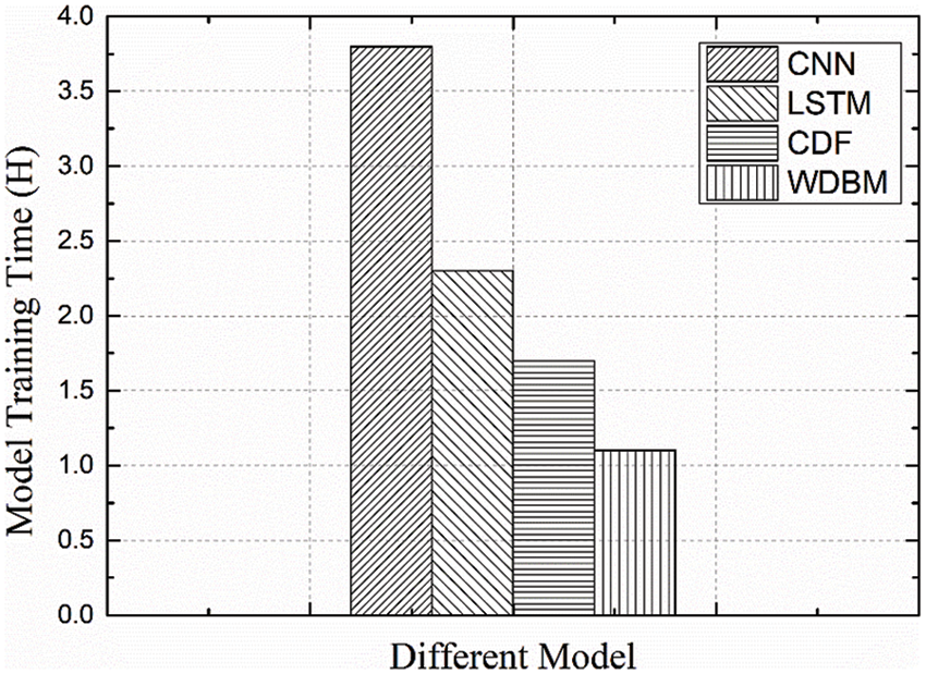
Figure 8: Model training time comparison of various diagnostic methods
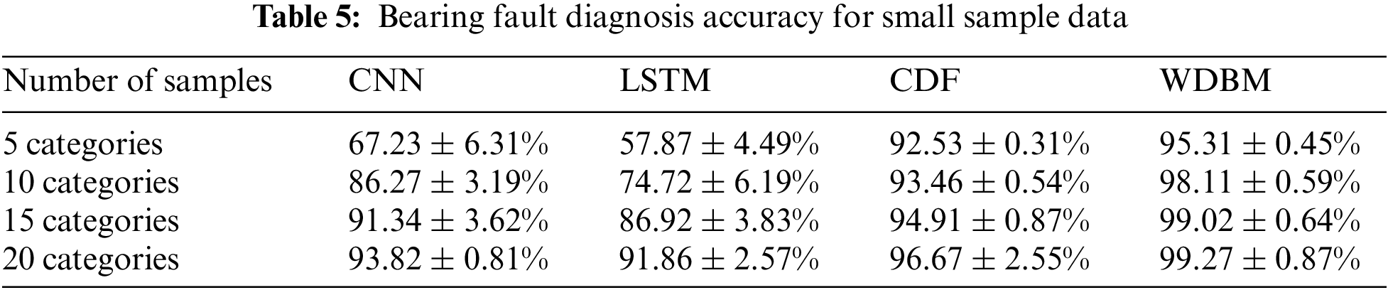
4.2.4 The Fault Diagnosis Performance Analysis for Small Sample Data
In this section, fault diagnosis experiments using small sample data are conducted to analyze the performance of the bearing fault diagnosis methods through the average fault diagnosis accuracy of 4 different types of small samples. The results are shown in Tab. 5. “5 categories” means that there is 1 category of healthy samples and 4 categories of fault samples when training the model and each type of sample contain 1000 data points, and so on. When 5 types of samples are used to train the model, the diagnosis rate of deep learning methods such as CNN and LSTM is seriously affected by the number of samples. When used 20 types of sample data, CNN increased by 26.59% and LSTM increased by 33.99%. For the tree-based model, CDF and WDBM are less affected by the sample data. When 5 types of small sample data are used, the diagnostic rate of CDF is 92.53%, and the precision rate of WDBM is 95.31%. The experimental results show that the number of training samples will affect the training effect of the model to some extent, and the possible reasons are as follows: For most deep learning methods, when sample data are relatively small, deep learning methods with more super parameters will produce serious over-fitting.
In engineering practice, the bearing is in normal operation for most of the time, combined with its working environment and other reasons, which make it difficult to obtain many real fault data samples. Therefore, fault diagnosis of small sample data sets is particularly important. In this paper, weighted deep forest is exploited for bearing fault diagnosis. The method has strong robustness, good generalization, and low cost. It can accurately diagnose on small data sets, and its accuracy rate is more than 99%, which can provide new power for bearing fault diagnosis technology.
Funding Statement: The work is supported by the National Key R&D Program of China (No. 2021YFB2700500, 2021YFB2700503). Tao Wang received the grant and the URLs to sponsors’ websites is https://service.most.gov.cn/.
Conflicts of Interest: The authors declare that they have no conflicts of interest to report regarding the present study.
1. R. N. Liu, B. Y. Yang, E. Zio and X. F. Chen, “Artificial intelligence for fault diagnosis of rotating machinery: A review,” Mechanical Systems and Signal Processing, vol. 108, no. 7, pp. 33–47, 2018. [Google Scholar]
2. B. Muruganatham, M. Sanjith, B. Krishnakumar and S. S. Murty, “Roller element bearing fault diagnosis using singular spectrum analysis,” Mechanical Systems & Signal Processing, vol. 35, no. 1–2, pp. 150–166, 2013. [Google Scholar]
3. Z. Dang, Y. Lv, Y. R. Li and G. Q. Wei, “Improved dynamic mode decomposition and its application to fault diagnosis of rolling bearing,” Sensors, vol. 18, no. 6, pp. 1–15, 2018. [Google Scholar]
4. J. X. Qu, Z. S. Zhang and T. Gong, “A novel intelligent method for mechanical fault diagnosis based on dual-tree complex wavelet packet transform and multiple classifier fusion,” Neurocomputing, vol. 171, no. 1, pp. 837–853, 2016. [Google Scholar]
5. D. T. Hoang and H. J. Kang, “A survey on deep learning based bearing fault diagnosis,” Neurocomputing, vol. 335, no. 3, pp. 327–335, 2019. [Google Scholar]
6. W. H. Li, R. Y. Huang, J. P. Li, Y. X. Liao, Z. Y. Chen et al., “A perspective survey on deep transfer learning for fault diagnosis in industrial scenarios: Theories, applications and challenges,” Mechanical Systems and Signal Processing, vol. 167, no. 3, pp. 1–15, 2022. [Google Scholar]
7. R. Jegadeeshwaran and V. Sugumaran, “Fault diagnosis of automobile hydraulic brake system using statistical features and support vector machines,” Mechanical Systems & Signal Processing, vol. 53, no. 2, pp. 436–446, 2015. [Google Scholar]
8. L. Sun, Y. Li, H. Du, P. P. Liang and F. S. Nian, “Fault diagnosis method of low noise amplifier based on support vector machine and hidden markov model,” Journal of Electronic Testing, vol. 37, no. 1, pp. 215–223, 2021. [Google Scholar]
9. P. Tamilselvan and P. Wang, “Failure diagnosis using deep belief learning based health state classification,” Reliability Engineering & System Safety, vol. 115, no. 7, pp. 124–135, 2013. [Google Scholar]
10. C. Lu, Z. Y. Wang and B. Zhou, “Intelligent fault diagnosis of rolling bearing using hierarchical convolutional network based health state classification,” Advanced Engineering Informatics, vol. 32, no. 4, pp. 139–151, 2017. [Google Scholar]
11. W. Zhang, G. L. Peng, C. H. Li, Y. H. Chen and Z. J. Zhang, “A new deep learning model for fault diagnosis with good anti-noise and domain adaptation ability on raw vibration signals,” Sensors, vol. 17, no. 2, pp. 425, 2017. [Google Scholar]
12. L. Eren, “Bearing fault eetection by one-dimensional convolutional neural networks,” Mathematical Problems in Engineering, vol. 2017, no. 8617315, pp. 1–9, 2017. [Google Scholar]
13. H. D. Yuan, J. Chen and G. M. Dong, “Bearing fault diagnosis based on improved locality-constrained Linear Coding and Adaptive PSO-Optimized SVM,” Mathematical Problems in Engineering, vol. 2017, no. 7257603, pp. 1–16, 2017. [Google Scholar]
14. X. Hao, Y. Zheng, L. Lu and H. Pan, “Research on intelligent fault diagnosis of rolling bearing based on improved deep residual network,” Applied Science, vol. 11, no. 22, pp. 1–14, 2021. [Google Scholar]
15. Z. H. Zhou and J. Feng, “Deep forest,” National Science Review, vol. 6, no. 1, pp. 74–86, 2019. [Google Scholar]
16. Y. J. Ren, K. Zhu, Y. Q. Gao, J. Y. Xia, S. Zhou et al., “Long-term preservation of electronic record based on digital continuity in smart cities,” Computers Materials & Continua, vol. 66, no. 3, pp. 3271–3287, 2021. [Google Scholar]
17. X. R. Zhang, X. Sun, X. M. Sun, W. Sun and S. K. Jha, “Robust reversible audio watermarking scheme for telemedicine and privacy protection,” Computers Materials & Continua, vol. 71, no. 2, pp. 3035–3050, 2022. [Google Scholar]
18. Y. L. Zhang, J. Zhou, W. H. Zheng, J. Feng, L. F. Li et al., “Distributed deep forest and its application to automatic detection of cash-out fraud,” ACM Transactions on Intelligent Systems and Technology, vol. 10, no. 5, pp. 1–19, 2019. [Google Scholar]
19. M. Huang, L. Z. Wang and Z. H. Zhang, “Improved deep forest mode for detection of fraudulent online transaction,” Computing and Informatics, vol. 39, no. 5, pp. 1082–1098, 2021. [Google Scholar]
20. C. Ma, Z. B. Liu, Z. G. Cao, W. Song, J. Zhang et al., “Cost-sensitive deep forest for price prediction,” Pattern Recognition, vol. 107, no. 11, pp. 1–16, 2020. [Google Scholar]
21. T. Li, Y. Ren and J. Xia, “Blockchain queuing model with non-preemptive limited-priority,” Intelligent Automation & Soft Computing, vol. 26, no. 5, pp. 1111–1122, 2020. [Google Scholar]
22. R. Su, X. Y. Liu, L. Y. Wei and Q. Zou, “Deep-Resp-Forest: A deep forest model to predict anti-cancer drug response,” Methods, vol. 166, no. 8, pp. 91–102, 2019. [Google Scholar]
23. Y. F. Zhu, S. Y. Fu, S. H. Yang, P. Liang and Y. Tan, “Weighted deep forest for schizophrenia data classification,” IEEE Access, vol. 8, no. 3, pp. 62698–62705, 2020. [Google Scholar]
24. L. Ren, J. Hu, M. Li, L. Zhang and J. Xia, “Structured graded lung rehabilitation for children with mechanical ventilation,” Computer Systems Science & Engineering, vol. 40, no. 1, pp. 139–150, 2022. [Google Scholar]
25. Y. D. Chen, A. Guo, Q. Q. Chen, B. Quan, G. Q. Liu et al., “Intelligent classification of antepartum cardiotocography model based on deep forest,” Biomedical Signal Processing and Control, vol. 67, no. 102555, pp. 1–8, 2021. [Google Scholar]
26. X. H. Cao, L. Wen, Y. M. Ge, J. Zhao and L. C. Jiao, “Rotation-based deep forest for hyperspectral imagery classification,” IEEE Geoscience and Remote Sensing Letters, vol. 16, no. 7, pp. 1105–1109, 2019. [Google Scholar]
27. Y. Ren, F. Zhu, J. Wang, P. Sharma and U. Ghosh, “Novel vote scheme for decision-making feedback based on blockchain in internet of vehicles,” IEEE Transactions on Intelligent Transportation Systems, vol. 23, no. 2, pp. 1639–1648, 2022. [Google Scholar]
28. X. B. Liu, R. L. Wang, Z. H. Cai, Y. M. Cai and X. Yin, “Deep multi-grained cascade forest for hyperspectral image classification,” IEEE Transactions on Geoscience and Remote Sensing, vol. 57, no. 10, pp. 8169–8183, 2019. [Google Scholar]
29. T. C. Zhou, X. B. Sun, X. Xia, B. Li and X. Chen, “Improving defect prediction with deep forest,” Information and Software Technology, vol. 114, no. 6, pp. 204–216, 2019. [Google Scholar]
30. Y. Ren, Y. Leng, J. Qi, K. S. Pradip, J. Wang et al., “Multiple cloud storage mechanism based on blockchain in smart homes,” Future Generation Computer Systems, vol. 115, no. 2, pp. 304–313, 2021. [Google Scholar]
31. L. V. Utkin, M. S. Kovalev and A. A. Meldo, “A deep forest classifier with weights of class probability distribution subsets,” Knowledge-Based Systems, vol. 173, no. 9, pp. 15–27, 2019. [Google Scholar]
32. X. R. Zhang, W. F. Zhang, W. Sun, X. M. Sun and S. K. Jha, “A robust 3-D medical watermarking based on wavelet transform for data protection,” Computer Systems Science & Engineering, vol. 41, no. 3, pp. 1043–1056, 2022. [Google Scholar]
 | This work is licensed under a Creative Commons Attribution 4.0 International License, which permits unrestricted use, distribution, and reproduction in any medium, provided the original work is properly cited. |