DOI:10.32604/cmc.2022.027364
| Computers, Materials & Continua DOI:10.32604/cmc.2022.027364 | |
| Article |
Experimental Analysis of Methods Used to Solve Linear Regression Models
1Computer Information Systems Department, The University of Jordan, Aqaba, 77110, Jordan
2Electrical Engineering Department, Al-Balqa Applied University, As Salt, 19117, Jordan
3Computers and Networks Engineering Department, Amman, 15008, Jordan
*Corresponding Author: Mua’ad Abu-Faraj. Email: m.abufaraj@ju.edu.jo
Received: 15 January 2022; Accepted: 24 March 2022
Abstract: Predicting the value of one or more variables using the values of other variables is a very important process in the various engineering experiments that include large data that are difficult to obtain using different measurement processes. Regression is one of the most important types of supervised machine learning, in which labeled data is used to build a prediction model, regression can be classified into three different categories: linear, polynomial, and logistic. In this research paper, different methods will be implemented to solve the linear regression problem, where there is a linear relationship between the target and the predicted output. Various methods for linear regression will be analyzed using the calculated Mean Square Error (MSE) between the target values and the predicted outputs. A huge set of regression samples will be used to construct the training dataset with selected sizes. A detailed comparison will be performed between three methods, including least-square fit; Feed-Forward Artificial Neural Network (FFANN), and Cascade Feed-Forward Artificial Neural Network (CFFANN), and recommendations will be raised. The proposed method has been tested in this research on random data samples, and the results were compared with the results of the most common method, which is the linear multiple regression method. It should be noted here that the procedures for building and testing the neural network will remain constant even if another sample of data is used.
Keywords: Linear regression; ANN; CFFANN; FFANN; MSE; training cycle; training set
In many engineering experiments, practical results are obtained that require finding the relationship between some of the inputs and outputs so that this relationship can be applied to find the output values depending on the input values without resorting to experiment and measurement provided that the output values are accurate and achievable at a very low error rate (very close to zero). The process of finding the relationship between the independent variables and the dependent ones (response) as shown in Fig. 1 is called solving the linear regression model (or linear prediction process) [1–5].
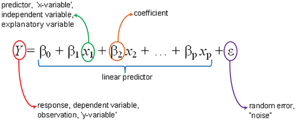
Figure 1: Linear regression (prediction) model [3]
Methods other than linear regression are used to approximate the solution of an equation for some system, in [6] they used two different techniques to compare the analytical solutions for the Time-Fractional Fokker-Plank Equation (TFFPE); including the new iterative method and the fractional power series method (FPSM). The experimental result shows that there is a good match between the approximated and the exact solution.
On the other hand, the relation between the target value and the predicting variables is non-linear in most cases. Therefore, more techniques that are sophisticated must be used in similar cases. In [7], the authors used the reduced differential transform method to solve the nonlinear fractional model of tumor immune. The obtained results show that the solutions generated for the nonlinear model are very accurate and simple.
The quality of any selected method to solve the linear regression model can be measured by Mean Square Error (MSE) and/or Peak Signal to Noise Ratio (PSNR), these quality parameters can be calculated using Eqs. (1) and (2) [8–12]:
S: experimental data
R: calculated data
The selected method is very accurate when the MSE value is very close to zero, or/and PSNR value is close to infinite [13–16]. The process of solving a linear regression model can be implemented as shown in Fig. 2 applying the following steps [17]:
Collect the experimental data of measurements.
Analyze the collected data and perform some filtering and normalization if needed.
Select a set of data samples to be used as a training dataset.
Select a method to solve the prediction problem.
Check MSE or PSNR, if they are acceptable then save the model solution to be used later in the prediction process, otherwise, increase the training dataset size, or modify some model parameters and retrain the model again.
The process of predicting the value of non-independent variables depending on a set of values of independent variables is a very important process due to its use in many applications and vital fields, including educational, medical, and industrial. The results of the prediction process are used to build future strategies and plans, and accordingly, the mathematical models used in the prediction process must provide very high accuracy to reduce as much as possible the error ratio between the calculated values and the expected values, and given the importance of the prediction process in decision-making, we will in this research paper by analyzing some mathematical models whose structure remains to some extent fixed even if the number of inputs and the number of outputs is changed.
All that matters to us in the research paper is the accuracy of the results and obtaining accurately calculated values that are very close to the expected values, and accordingly, it was sufficient to use MSE and/or PSNR.
The Linear regression model can be solved in a simple way using arithmetic calculations (least square fit method) [18,19], the solution of the model will find the regression coefficients as shown in Fig. 2.
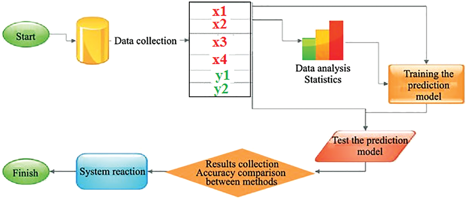
Figure 2: Solving prediction model [14]
Here, the process of linear regression solution using a simple example is being described; this example will be solved using MATLAB. If we consider the following regression problem shown in Fig. 3:
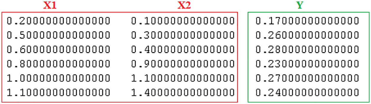
Figure 3: Linear regression example
To calculate the regression coefficients, we must apply the following steps:
1. Generate a regression matrix that includes the independent variables values, the elements of the first column of this matrix must equal to one as shown in Fig. 4:
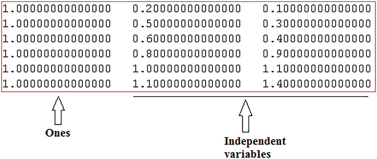
Figure 4: Regression matrix
2. Use the backslash operator in MATLAB to divide the regression matrix by the output matrix, for this example we will get the values of the following coefficients, as depicted in Fig. 5:
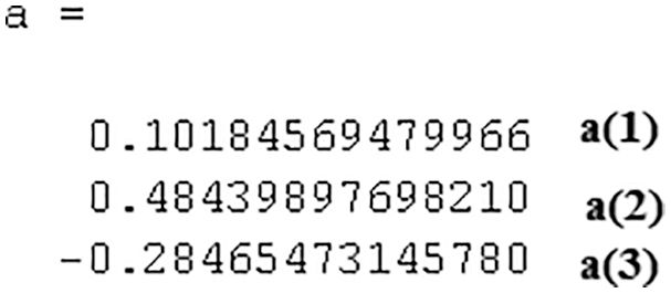
Figure 5: Coefficient values
3. Use the regression coefficients to construct the output equation according to Eq. (3):
4. Now we can apply Eq. (3) to predict the value of y for any given values of x1 and x2.
Fig. 6 shows the experimental and predicted outputs for this example, the predicted values are very close to the true values for all the samples. It is expected since the dataset is very small and the least square fit works efficiently with such a dataset. However, this method usually gives high MSE values, especially, when the size of experimental data is big, this will be discussed later in Section 4.
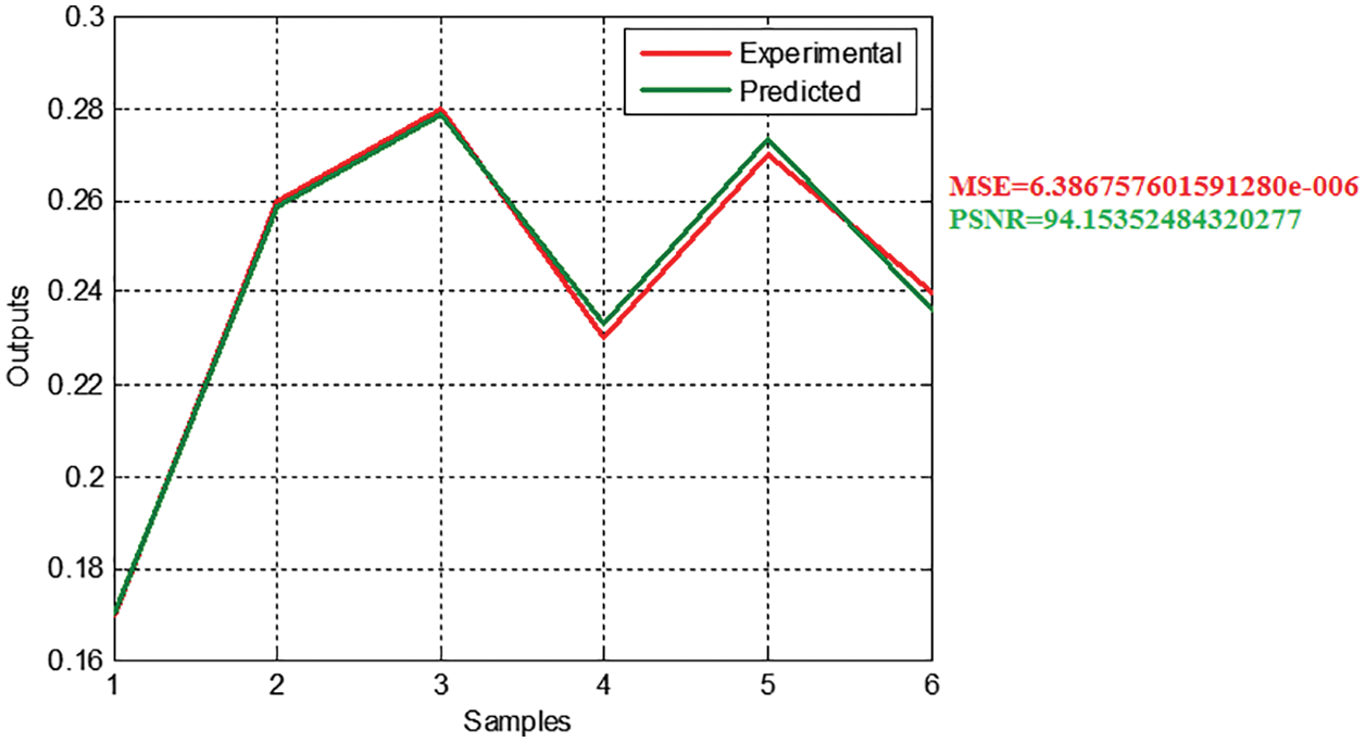
Figure 6: Experimental and predicted outputs (example)
An Artificial neural network (ANN) is a powerful computational model that consists of a set of fully connected neurons organized in one or more layers [20–23]. Each neuron is a computational cell that performs two main operations as shown in Fig. 7.
An activation function must be assigned for each layer and each neuron in this layer, the output of the neuron will be calculated depending on the assigned activation function, for linear activation function the neuron output will equal the summation, while for logsig and tansig activation functions the output of the neuron will be calculated as shown in Fig. 8.
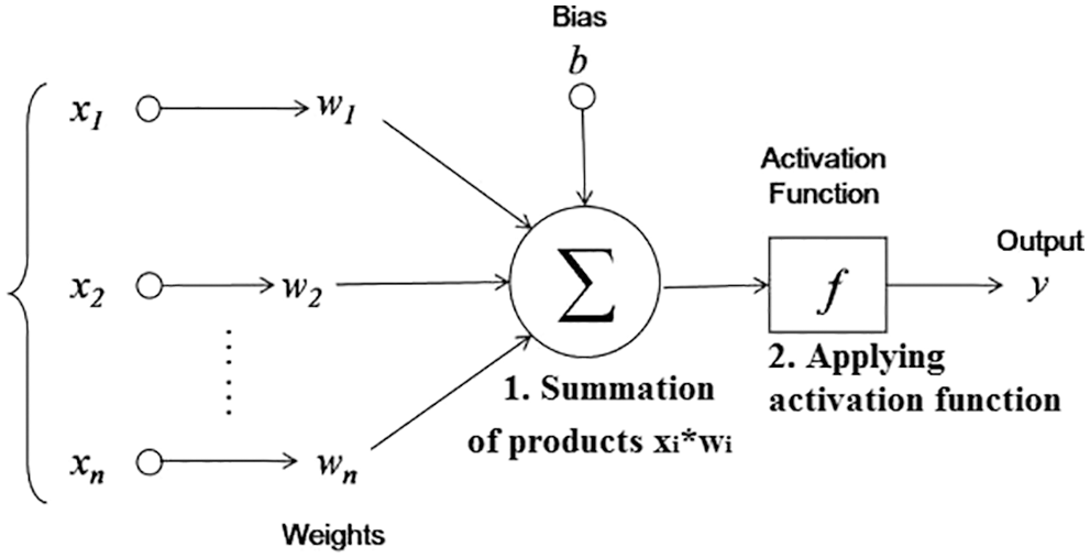
Figure 7: Neuron operation [12]
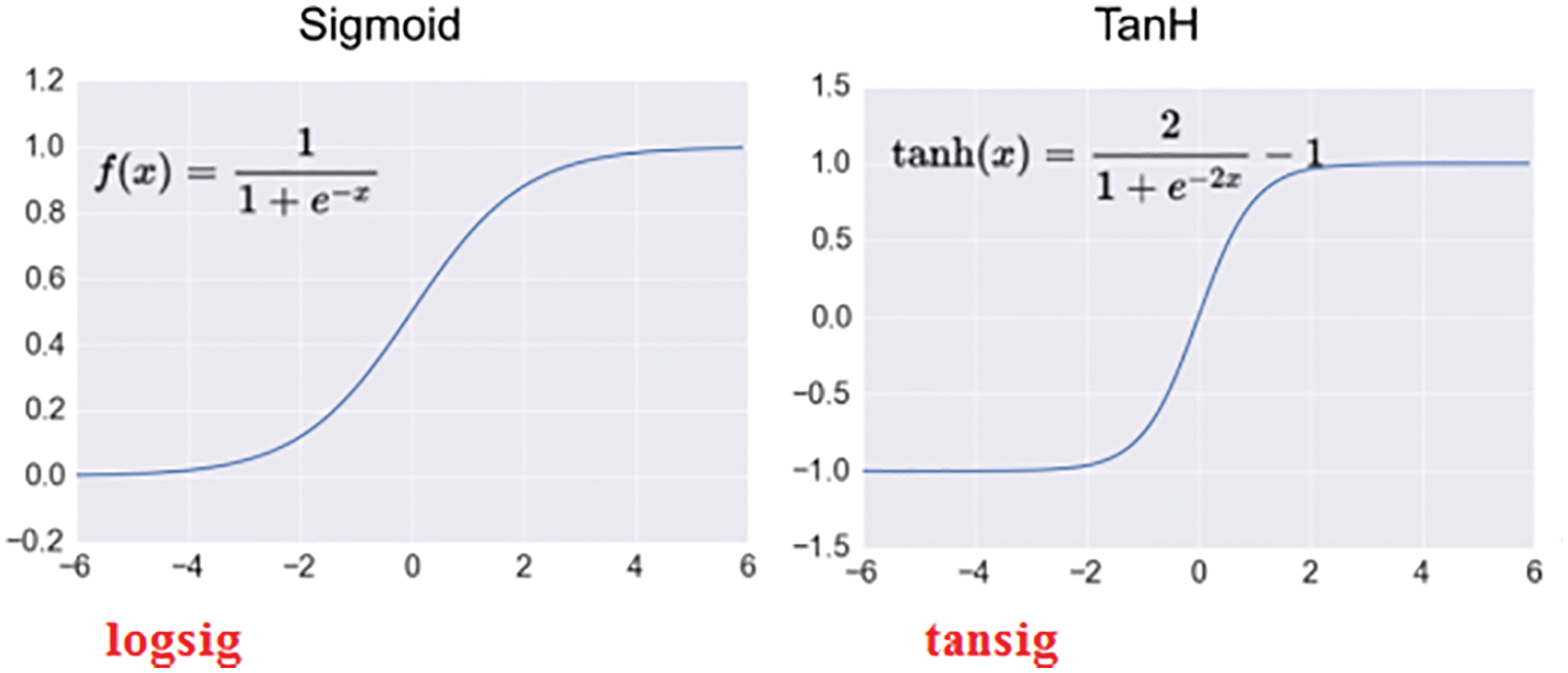
Figure 8: Neuron output calculation using logsig (Sigmoid) and tansig (TanH) activation functions
ANN can be easily used in many applications including solving linear regression models by directly predicting the output values using the input variable values as an input for the ANN. ANN model can be treated as a black box, with selected inputs and the outputs to be predicted. A set of samples from the input data must be selected as training samples, these samples are used to train ANN, the results of training must give an acceptable value of MSE, so selecting the size of training samples and the number of training cycles will affect ANN performance. Each training cycle computes the neuron outputs starting from the ANN input layer, then the final calculated outputs are compared with target outputs by computing MSE between them, if the MSE value is acceptable then the computation will be stopped, otherwise, backpropagation calculations will be performed starting from the output to find the errors and make a necessary weight updating as shown in Figs. 9 and 10.
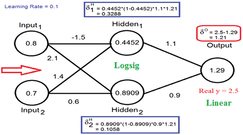
Figure 9: Neuron outputs calculation
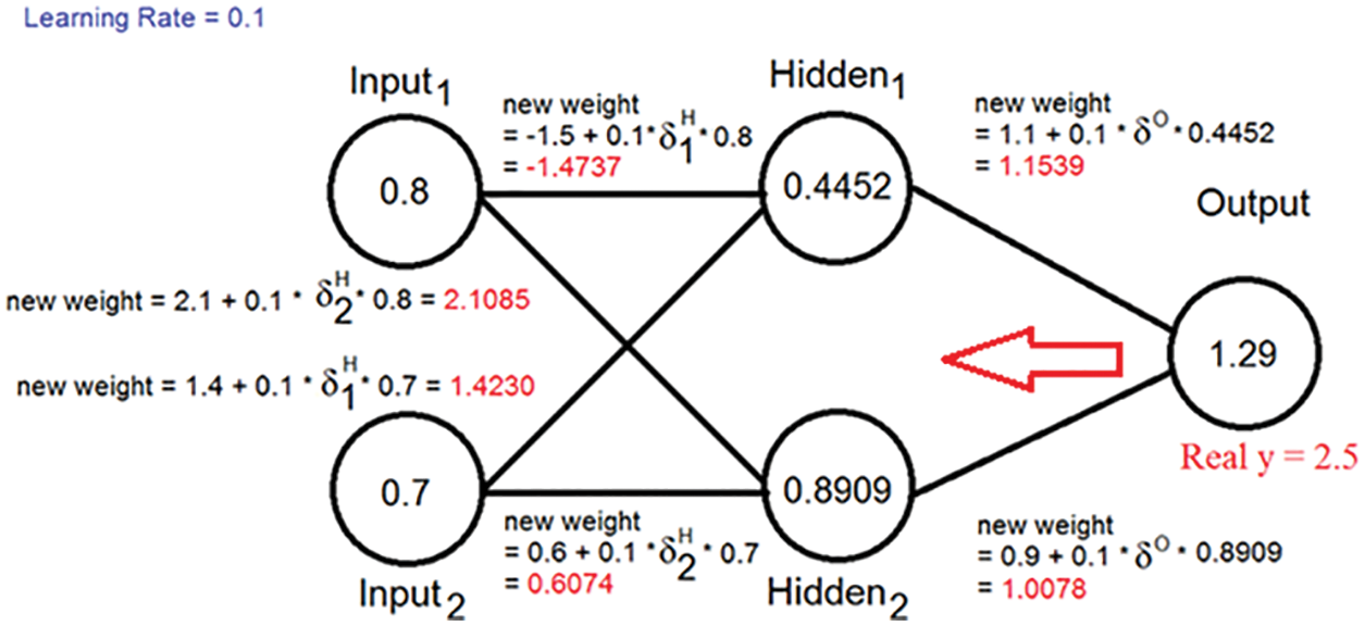
Figure 10: Error calculations and weights updating
The process of using ANN as a prediction tool can be summarized in the following steps:
Step 1: Data preparation from the collected data we must select several samples which include the independent variables values and the measured outputs (true labels to be predicted), these values must be organized in a matrix, one column for each sample value, the input data must be normalized to avoid error in the results of logsig or tansig calculations (see Fig. 11).
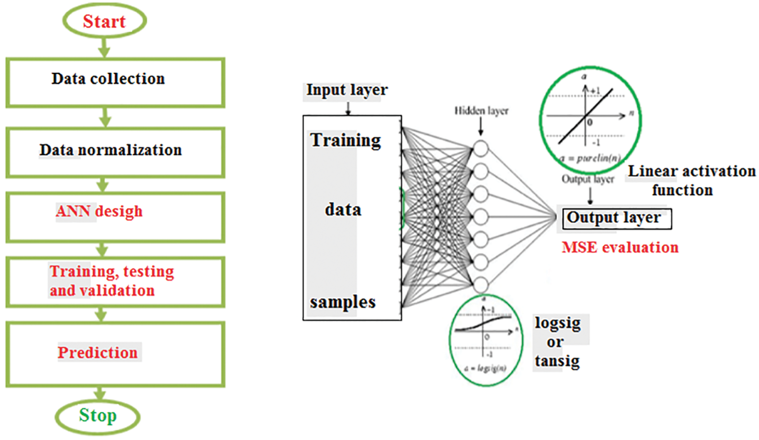
Figure 11: ANN presentation [16]
Step 2: ANN creation and design in this step we must create an ANN architecture by selecting the number of layers and the number of neurons in each layer, an activation function must be assigned to each layer. The goal (acceptable MSE) and the number of training cycles must be determined (see Fig. 12). ANN must be initialized and trained using the inputs and the target labels to be predicted.
After finishing each training cycle MSE will be computed and compared with the goal, if the error is acceptable, we can save the net to be used as a prediction tool, otherwise, we must increase the number of training cycles, or update ANN architecture and retrain it again.
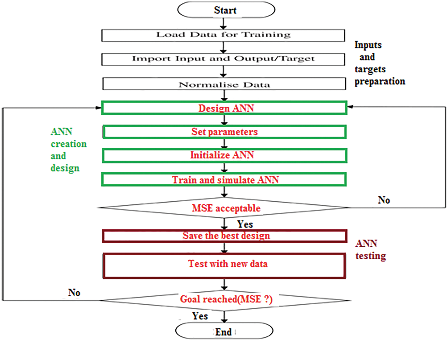
Figure 12: ANN design and testing [16]
Step 3: ANN testing A set of new samples is selected for testing purposes, the saved ANN model is run and loaded with the test samples. MSE is calculated between the true values for the test samples and the predicted labels by the ANN model. If the computed value of MSE is acceptable, then ANN can be used in the future to predict any values of the outputs given the necessary inputs, otherwise, ANN must be modified and retrained again.
4 Implementation and Experimental Results
5000 samples of two independent variables and one dependent variable were selected. The linear regression model was solved using MATLAB, the size of training samples dataset size was varied from 100 to 2000 samples. The regression coefficients were computed for each training set of samples, then the predicted outputs were calculated using the associated regression equations, the expected MSE for each case was calculated, Tab. 1 lists the obtained experimental results, MSE values are almost stable regardless of the training set size.
Now we will use the same samples to train and test ANN, and here two types of ANN architectures are selected, including Feed-Forward ANN (FFANN) and Cascade Feed-Forward ANN (CFFANN), the differences between these two types of ANN are shown in Fig. 13 [24–26].
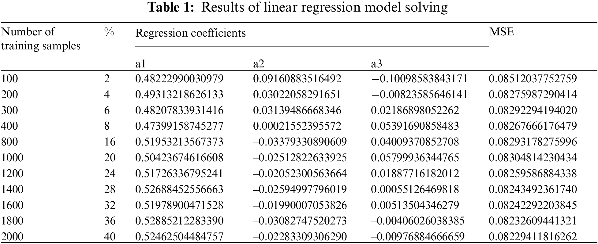
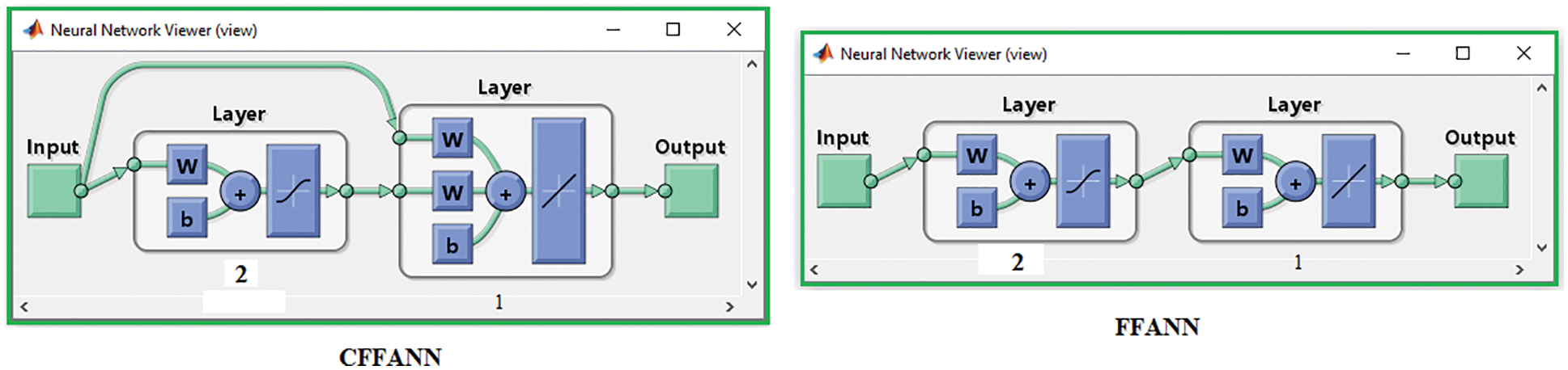
Figure 13: CFFANN and FFANN architectures
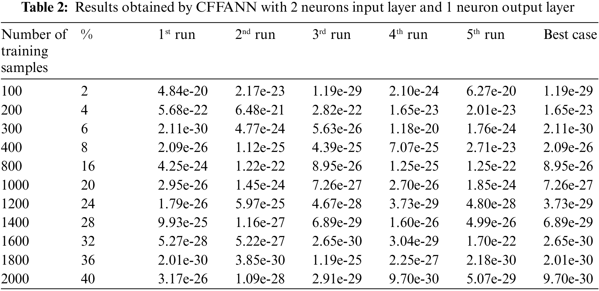
The optimal architecture of the selected ANN consists of one input layer with 2 neurons and 1 output layer with 1 neuron. CFFANN with the selected architecture was trained and tested; Tab. 2 lists the obtained results (for each training set ANN was run five times and the best case was selected).
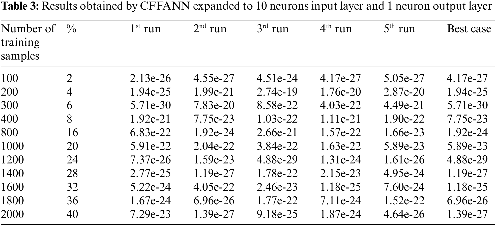
The architecture of CFFANN was updated by expanding the number of neurons in the input layer to 12, Tab. 3 lists the obtained results. The same experiment was repeated using CFFANN with a hidden layer of 4 neurons, Tab. 4 lists the results for this ANN.
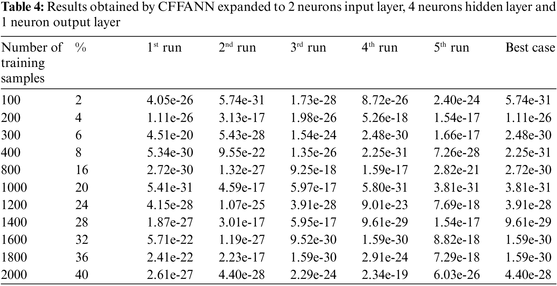
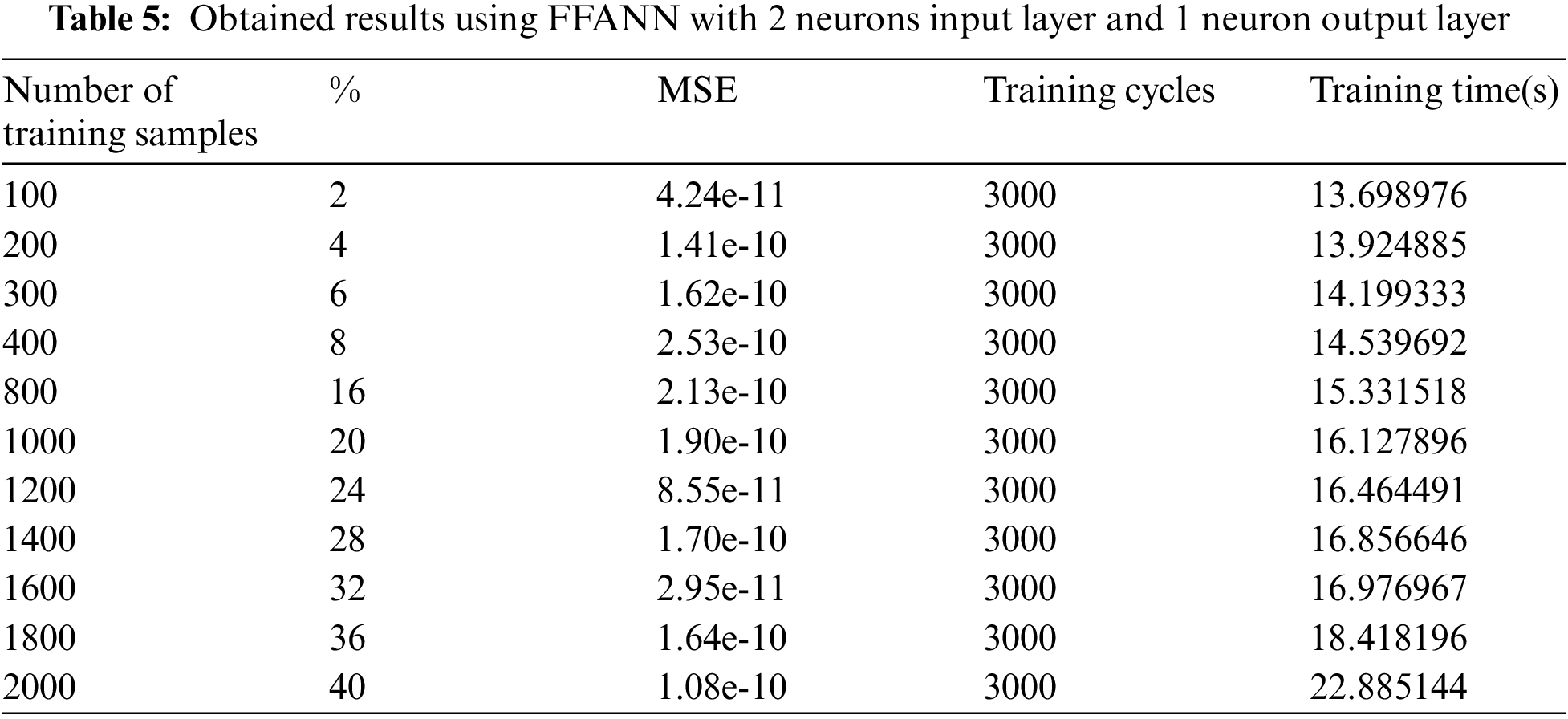
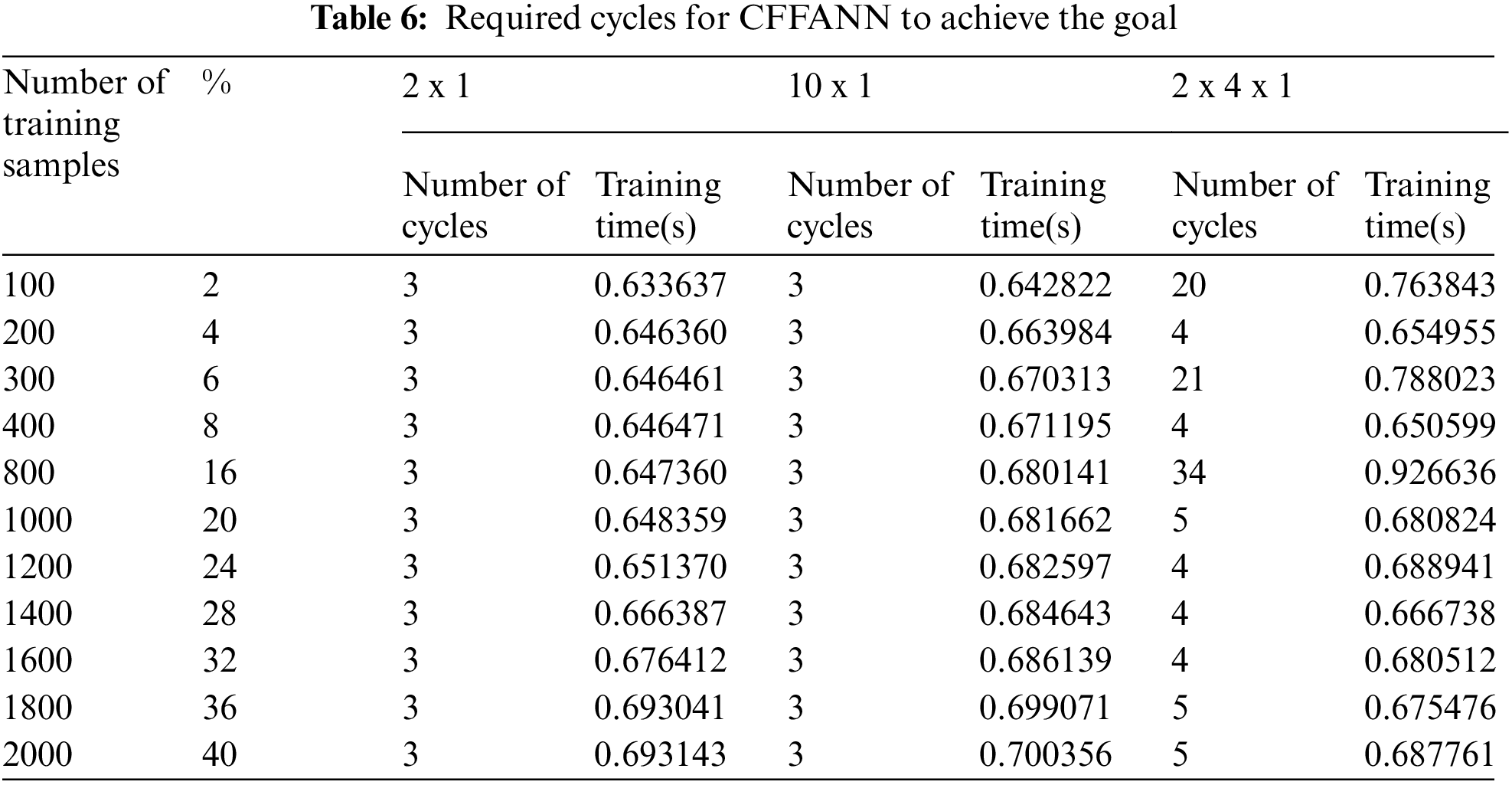
In the previous experiments, the selected number of training cycles was equal to 3000 cycles, FFANN with minimal architecture was trained and tested, and Tab. 5 lists the obtained results, while Tab. 6 shows the required training cycles to achieve the goal for CFFANN with different architectures.
Solving the regression model using the least square fit method shows very poor results, the calculated MSE between the targets and the calculated outputs using regression coefficients was always high regardless of the training sample size, as depicted in Figs. 14 and 15.
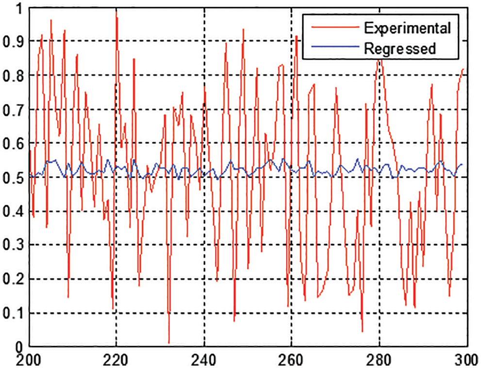
Figure 14: Experimental and predicted outputs using least square fit method
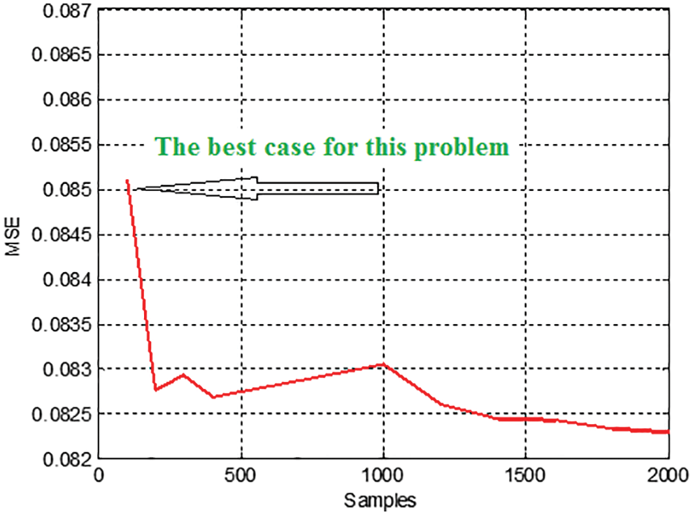
Figure 15: Computed MSE using various training sets
To overcome the disadvantages of the least square fit method, ANN is introduced as a prediction tool in two different flavors, which are FFANN and CFFANN. Using FFANN architecture increases the quality of the linear regression solving, but it requires many training cycles and training time (as listed in Tab. 5), expanding the number of neurons in the input layer or adding an extra hidden layer does not improve the value of MSE (see Fig. 16).
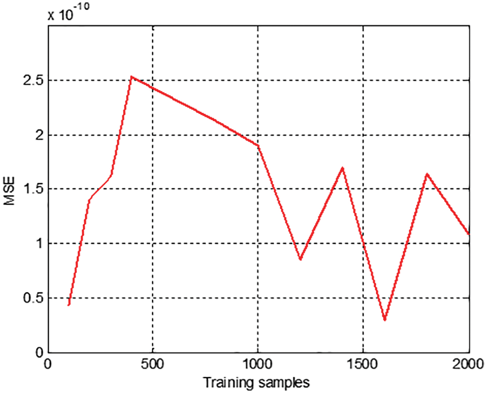
Figure 16: Calculated MSE using FFANN
To improve the performance of the ANN model, it is better to use CFFANN. The main advantages of using CFFANN compared to FFANN are that it needs a smaller number of training cycles, and it can achieve the goal of minimal MSE value. Moreover, A small set of training samples can be used to train CFFANN; this ANN can be saved and easily used to predict the output using any given inputs, the output that is generated using CFFANN is much closer to the target with an MSE value closer to zero as shown in Fig. 17.
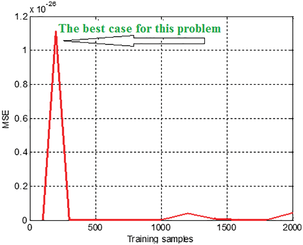
Figure 17: Calculated MSE using FFANN
Several methods were implemented to solve the linear regression model, the least square fit method was used to find the regression coefficients, and these coefficients then were used to construct the regression equation, which was used to calculate the predicted output. The least square method showed the poorest results even if the set of training samples size was increased. To overcome the disadvantages of the least square method, various models of ANN were proposed, which include: FFANN and CFFANN. The obtained experimental results showed that CFFANN with any architecture and with various sizes of the training set achieved the best performance by minimizing the number of training cycles required to achieve the minimum MSE value. Thus, the CFFANN model is highly recommended to solve the linear regression model.
Recommendation: The proposed procedure will still be stable even if we use another sample of data, a simple modification of ANN architecture is required to match the number of inputs and the number of targets to be calculated.
Funding Statement: The authors received no specific funding for this study.
Conflicts of Interest: The authors declare that they have no conflicts of interest to report regarding the present study.
1. A. Abraham, F. Pedregosa, M. Eickenberg, P. Gervais, A. Mueller et al., “Machine learning for neuroimaging with scikit-learn,” Frontiers in Neuroinformatic, vol. 8, pp. 14, 2014. [Google Scholar]
2. S. Albawi, T. A. Mohammed and S. Al-Zawi, “Understanding of a convolutional neural network,” in Int. Conf. on Engineering and technology (ICET) 1-6, Antalya, Turkey, pp. 1–6, 2017. [Google Scholar]
3. J. Antonakis, N. Bastardoz and M. Rönkkö, “On ignoring the random effects assumption in multilevel models: Review, critique, and recommendations,” Organizational Research Methods, vol. 24, no. 2, pp. 443–483, 2021. [Google Scholar]
4. C. B. Azodi, J. Tang and S. H. Shiu, “Opening the black box: Interpretable machine learning for genetics,” Trends in Genetics, vol. 36, no. 6, pp. 442–455, 2020. [Google Scholar]
5. E. Barends and D. M. Rousseau, “Evidence-Based Management: How to Use Evidence to Make Better Organizational Decisions,” New York, NY: Kogan Page Publishers, 2018. [Google Scholar]
6. A. M. Mahdy, “Numerical solutions for solving model time-fractional Fokker-Planck equation,” Numerical Methods for Partial Differential Equations, vol. 37, no. 2, pp. 1120–1135, 2021. [Google Scholar]
7. A. M. Mahdy, M. Higazy and M. S. Mohamed, “Optimal and memristor-based control of a nonlinear fractional tumor-immune model,” Computers, Materials & Continua, vol. 67, no. 3, pp. 3463–3486, 2021. [Google Scholar]
8. A. Bell, M. Fairbrother and K. Jones, “Fixed and random effects models: Making an informed choice,” Quality & Quantity, vol. 53, no. 2, pp. 1051–1074, 2019. [Google Scholar]
9. P. D. Bliese, D. Chan and R. E. Ployhart, “Multilevel methods: Future directions in measurement, longitudinal analyses, and nonnormal outcomes,” Organizational Research Methods, vol. 10, no. 4, pp. 551–563, 2007. [Google Scholar]
10. L. Breiman, “Bagging predictors,” Machine Learning, vol. 24, no. 2, pp. 123–140, 1996. [Google Scholar]
11. L. Breiman, “Random forests,” Machine Learning, vol. 45, no. 1, pp. 5–32, 2001. [Google Scholar]
12. L. Breiman, J. H. Friedman, R. A. Olshen and C. J. Stone, “Classification and regression trees,” Routleadge, 2017. [Google Scholar]
13. L. Capitaine, R. Genuer and R. Thiébaut, “Random forests for high-dimensional longitudinal data,” Statistical Methods in Medical Research, vol. 30, no. 1, pp. 166–184, 2021. [Google Scholar]
14. P. Choudhury, R. T. Allen and M. G. Endres, “Machine learning for pattern discovery in management research,” Strategic Management Journal, vol. 42, no. 1, pp. 30–57, 2021. [Google Scholar]
15. J. A. Cobb and K. H. Lin, “Growing apart: The changing firm-size wage premium and its inequality consequences,” Organization Science, vol. 28, no. 3, pp. 429–446, 2017. [Google Scholar]
16. A. C. Davison and D. V. Hinkley, “Bootstrap Methods and Their Application,” Cambridge: Cambridge University Press, 1997. [Google Scholar]
17. M. Deen and M. de Rooij, “ClusterBootstrap: An R package for the analysis of hierarchical data using generalized linear models with the cluster bootstrap,” Behavior Research Methods, vol. 52, no. 2, pp. 572–590, 2020. [Google Scholar]
18. A. Fisher, C. Rudin and F. Dominici, “All models are wrong, but many are useful: Learning a variable's importance by studying an entire class of prediction models simultaneously,” Journal of Machine Learning Research, vol. 20, no. 177, pp. 1–81, 2019. [Google Scholar]
19. J. Fox, “Applied Regression Analysis and Generalized Linear Models,” London: SAGE Publications, 2015. [Google Scholar]
20. P. J. García-Laencina, J. L. Sancho-Gómez and A. R. Figueiras-Vidal, “Pattern classification with missing data: A review,” Neural Computing & Applications, vol. 19, no. 2, pp. 263–282, 2010. [Google Scholar]
21. S. Garg, S. Sinha, A. K. Kar and M. Mani, “A review of machine learning applications in human resource management,” International Journal of Productivity and Performance Management, vol. 63, no. 3, pp. 308, 2021. [Google Scholar]
22. J. Grimmer, M. E. Roberts and B. M. Stewart, “Machine learning for social science: An agnostic approach,” Annual Review of Political Science, vol. 24, no. 1, pp. 395–419, 2021. [Google Scholar]
23. E. L. Hamaker and B. Muthén, “The fixed versus random effects debate and how it relates to centering in multilevel modelling,” Psychological Methods, vol. 25, no. 3, pp. 365, 2020. [Google Scholar]
24. M. Hausknecht, W. K. Li, M. Mauk and P. Stone, “Machine learning capabilities of a simulated cerebellum,” IEEE Transactions on Neural Networks and Learning Systems, vol. 28, no. 3, pp. 510–522, 2016. [Google Scholar]
25. M. A. Hearst, S. T. Dumais, E. Osuna, J. Platt and B. Scholkopf, “Support vector machines,” IEEE Intelligent Systems and Their Applications, vol. 13, no. 4, pp. 18–28, 1998. [Google Scholar]
26. Y. C. Ho and D. L. Pepyne, “Simple explanation of the no-free-lunch theorem and its implications,” Journal of Optimization Theory and Applications, vol. 115, no. 3, pp. 549–570, 2002. [Google Scholar]
 | This work is licensed under a Creative Commons Attribution 4.0 International License, which permits unrestricted use, distribution, and reproduction in any medium, provided the original work is properly cited. |