Computers, Materials & Continua DOI:10.32604/cmc.2022.027400
Article

Multi-Target Track Initiation in Heavy Clutter

Li Xu1,2,*, Ruzhen Lou1, Chuanbin Zhang1, Bo Lang3 and Weiyue Ding4

1College of Computer Science and Technology, Harbin Engineering University, Harbin, 150001, China
2Key Laboratory of Symbolic Computation and Knowledge Engineering of Ministry of Education, Jilin University, Changchun, 130012, China
3Norinco Group Air Ammunition Research Institute Co. Ltd., Harbin, 150036, China
4Harvard Medical School, Boston, 02115, USA
*Corresponding Author: Li Xu. Email: xuli@hrbeu.edu.cn
Received: 17 January 2022; Accepted: 04 March 2022

Abstract: In the heavy clutter environment, the information capacity is large, the relationships among information are complicated, and track initiation often has a high false alarm rate or missing alarm rate. Obviously, it is a difficult task to get a high-quality track initiation in the limited measurement cycles. This paper studies the multi-target track initiation in heavy clutter. At first, a relaxed logic-based clutter filter algorithm is presented. In the algorithm, the raw measurement is filtered by using the relaxed logic method. We not only design a kind of incremental and adaptive filtering gate, but also add the angle extrapolation based on polynomial extrapolation. The algorithm eliminates most of the clutter and obtains the environment with high detection rate and less clutter. Then, we propose a fuzzy sequential Hough transform-based track initiation algorithm. The algorithm establishes a new meshing rule according to system noise to balance the relationship between the grid granularity and the track initiation quality. And a flexible superposition matrix based on fuzzy clustering is constructed, which avoids the transformation error caused by 0–1 voting method in traditional Hough transform. In addition, the algorithm allows the superposition matrixes of nonadjacent cycles to be associated to overcome the shortcoming that the track can’t be initiated in time when the measurements appear in an intermittent way. And a slope verification method is introduced to detect formation-intensive serial tracks. Last, the sliding window method is employed to feedback the track initiation results timely and confirm the track. Simulation results verify that the proposed algorithms can initiate the tracks accurately in heavy clutter.

Keywords: Track initiation; heavy clutter; multi-target; Hough transform

1  Introduction

In the early stage of target tracking, the measurement cycles of the detection system are limited. Track initiation is to select the stable and reliable tracks from the limited measurement cycles. As the first step in target tracking [1], the quality of track initiation (TI) affects all subsequent stages of target tracking.

Due to the importance of track initiation and its broad application in military and civil fields [2], it has been highly concerned by scholars and engineering experts. A lot of significant works on the track initiation problem have been done. In particular, many researches were focused on the problem in challenging scenarios, such as the harsh underwater target tracking environment [3], multiple maneuvering targets hidden in the Doppler blind zone [4], dense clutter environment [5–7], a very noisy background [8] and so on.

At the same time, scholars have put forward a variety of solutions to the track initiation problem under different conditions, for instance, narrowband target tracking situation [9], a low observable target with multipath measurements [10], closely spaced objects in the presence of clutter [11], the new target appearing in the detected area Luo et al. [12]. These conditions are much closer to the real world, and the track initiation problem under these conditions becomes more complex.

In addition, over the last few years, scholars have studied track initiation problem from different perspectives. The following is a summary of the typical recent works. Liu et al. [13] present a novel method based on the random forest to address the problem of track initiation in the air-traffic-control radar system. Lee et al. [14] introduce a track initiation algorithm based on the weighted score for TWS radar tracking. Jiang et al. [15] improve the Bayesian group track initiation algorithm based on algebraic graph theory. Baek et al. [16] develop a computationally efficient track initiation method for multi-static multi-frequency passive coherent localization systems, where bistatic measurements from different illuminators are incorporated at a receiver to find the most probable track initiation points. Wilthil et al. [17] derive a Bayesian SPRT for track initiation based on Reid’s multiple hypothesis tracker. Liu et al. [18] apply the rule-based track initiation technique to the Gaussian mixture PHD filter, and propose the Gaussian mixture PHD filter with track initiation. Hunde et al. [19] discuss a multi-target tracking system that addresses target initiation and termination processes with automatic track management feature. Vaughan et al. [20] conduct a statistical analysis that yields an accurate approximation of the false-track and track detection probabilities as a function of the threshold on the track-initiation statistic. Han et al. [21] propose a novel track initiation algorithm based on agglomerated hierarchical clustering and association coefficients. These works all contribute to the research of the track initiation problem.

In the heavy clutter and multi-target environment [22], the information capacity is large, the relationships among information are complicated [23,24], the number of the detected targets is unknown [25], and track initiation often has a high false alarm rate or missing alarm rate. Obviously, it is still a difficult task to get a high-quality track initiation in the limited measurement cycles [26–28]. Therefore, multi-target track initiation in heavy clutter is a challenging and significant task [29,30].

The paper researches key problems of track initiation in heavy clutter, and gives the corresponding solutions. There are two aspects as follows. At first, we present a relaxed logic-based clutter filter algorithm (RLCF), which is to eliminate most of the clutter and to obtain the environment with high detection rate and less clutter. In the following, a fuzzy sequential Hough transform-based track initiation algorithm (FSHTTI) is proposed, which has higher accuracy and stronger suppression ability of false track. Simulation results verify that the proposed algorithms can initiate the tracks accurately and solve the following key problems effectively: clutter filter and track initiation in the heavy clutter and multi-target environment.

2  A Relaxed Logic-based Clutter Filter Algorithm

2.1 Design of Adaptive Gate

The size and number of wave gates are positively correlated with the success rate of track initiation. With the gradual increase of detection cycle, under the condition of the same number and size of wave gates, the probability of real point traces of the targets falling into wave gates gradually decreases. And considering the intermittent flicker of the measurements, the paper designs the adaptive wave gate.

Let the state of the detected target in cycle kri(k) be [hx(k),vx(k),hy(k),vy(k)]T, where, hx(k) and hy(k) represent the position of the target in the x-axis and y-axis respectively, and vx(k) and vy(k) represent the velocity of the target in the x-axis and y-axis respectively.

The measurement at the root lacks prior knowledge and cannot judge its motion information. The annular gate should be established according to the maximum and minimum velocity of the target. The inner diameter R1 and outer diameter R2 of the gate should meet the following requirements:

R1=vminT−w(1)

R2=vmaxT+w(2)

where, vmin and vmax are the minimum velocity and the maximum velocity of the target respectively. T is the time length of detection, and w is the root mean square of the system noise.

When a measurement has formed a temporary track, its measurement sequence is defined as Ri={ri(0),ri(1),ri(2)…}. (The track participating in the track confirmation screening is called candidate track. However, the logic method which is used for clutter filtering doesn’t include the process of track confirmation, so the track formed by this process is called temporary track). The gate form is determined by the measurement state. When the maneuverability of the target is weak, the sector ring gate is used.

Let vw be the turning angular velocity of the detected target. |ef| is the fan ring radius as shown in (3):

|ef|=(vmax−vmin)T+(amax−amin)T22+w(3)

α=vwT(4)

in which, the restrictions are as follows:

|ef|≤mσl(k)(5)

α≤nσθ(k)(6)

where, m and n are the coefficient, which can be set by the query table with χ2 distribution. σl(k) and σθ(k) are the standard deviation of radial distance and observation angle.

When the target maneuvering is enhanced, the real trace points of the targets are easy to fall out of the sector ring gate. At this time, the adaptive sector ring gate will reduce the detection probability of the real trace points and should be expanded. Because the detection system is far away from the targets and the tracks are approximately the straight line, the acceleration changes more sharply than the observation angle when the target maneuvers. Therefore, the expanded gate is closer to the ellipse.

The major axis of the ellipse is on the same line as the temporary track, whose length is:

a=2(vmax−vmin)T+(amax−amin)T2+2w(7)

The length of the minor axis is:

b=[(vmin+vmax)T+32(amax+amin)T2]tan(απ180)+2w(8)

r(k)=[rx(k),ry(k)]T represents the description of the ith measurement in the rectangular coordinate system in cycle k. The innovation is:

I(k+1)=r(k+1)−r^(k+1|k)=[rx(k+1)−rx^(k+1|k)ry(k+1)−ry^(k+1|k)](9)

where, r^(k+1|k) is extrapolation measurement. The innovation variance is:

S(k+1)=H(k+1)P(k+1|k)HT(k+1)+w1(k)(10)

where, P(k+1|k) is one-step prediction of covariance. If ri(k) satisfies:

V~k+1(γ)=I(k+1)TS−1(k+1)I(k+1)≤γ(11)

then it is considered that the measurement falls into the elliptical gate region. And the parameter γ can be obtained by querying the distribution table with χ2.

|ab|=(vmax+vmin)T2+(amax+amin)T24(12)

|ac|=(vmax+vmin)T+4(amax+amin)T24(13)

|ad|=3(vmax+vmin)T2+9(amax+amin)T24(14)

The distance from α to the extrapolation point in cycle k can be obtained:

d=(k−1)(vmax+vmin)T2+(k−1)2(amax+amin)T24(15)

When the target moves at a constant speed, the acceleration is 0, then:

d=(k−1)|ab|(16)

The radius of fan ring is constrained by Eqs. (1) and (2), and the length of ellipse axis is constrained by Eqs. (7) and (8), which increases adaptively as Eqs. (16). After extrapolation, if no measurements are detected in the corresponding adaptive gate, it is concluded that there is flicker discontinuity at this cycle. To improve the detection rate of trace points, this algorithm allows the temporary tracks with flicker discontinuity to participate in the extrapolation expansion of the next cycle. If there is no continuous flicker discontinuity, only the cycle with flicker discontinuity needs to be recorded. Otherwise, the temporary tracks will be cancelled.

2.2 Improvement of Extrapolation Extension

The way of extrapolation expansion affects the storage space and accuracy of the initiation algorithm. The logic extrapolation expansion generally adopts polynomial extrapolation in the form of straight line. However, considering the maneuverability of the targets, the large distance between the extrapolation points and the real trace points, and the angle deviation, the candidate tracks are extended by modifying the observation angles of the extrapolation points.

Let θi(k) is the observation angle of the ith extrapolated track in cycle k. Then before cycle k, all observation angles of the extrapolated tracks are:

θi={θi(0),θi(1),θi(2),…,θi(k)}(17)

If the target is moving in a straight line, there is:

θi(0)=θi(1)=θi(2)=…=θi(k)(18)

Due to the influence of target maneuverability and system noise, the measurements of detection system are often in non-linear form. So, the initial accuracy is low, if (17) is used as the extrapolation standard. According to the state equation, let:

θi(k+1)=αθi(k)+βw(k)(19)

where, α and β are the coefficient. w(k) is a Gaussian distribution with independent zero mean.

Let θi^(k) is the observation angle of the extrapolation point of the ith candidate track in cycle k. θi(sub)(k) is the difference between the observation angle of cycle 𝑘 and cycle 𝑘−1, then:

θi(sub)(k)=θi(k)−θi(k−1)=αθi(k−1)+βw(k−1)+θi(k−1)(20)

The extrapolation method with the observation angle as the influencing factor is expressed as follows:

θ^i(k+1|k)=θi(k)+θi(sub)(k)(21)

Let ri(0)∈R(0), the initial association region of ri(0) is Ω1 and ri(1)∈R(1)∩Ω1, then ri(1) is initial association measurement of ri(0). If the subsequent association region of ri(0) is Ωk, then r^i(k) is the central extrapolation point of Ωk.

According to the nearest neighborhood:

Ωk′={x∈R(k)∩Ωk|l(r^l(k|k−1),x)=miny∈R(k)∩Ωkl(r^l(k|k−1),y)}(22)

in which:

l(x,y)=max[0,x−y−vmaxt]+max[0,y−x+vmaxt](23)

Then, ri(k)∈Ωk, is called the kth association measurement of ri(0), all the possibilities are expressed as:

{ri(0),ri(1),ri(2)∈Ω2,…ri(N−1)∈ΩN−1,}(24)

The association measurement sequence of ri(0) is called the candidate track which takes ri(0) as the root. Only the measurements nearest to the predicted trace points shall be extrapolated next time.

According to the split expansion:

Ωk,={x∈R(k)∩Ωk}(25)

All the measurements with ri(k)∈Ωk′ are associated with the trace points of ri(0). To split association, we expand all measurements and extrapolate next time. And it needs a lot of storage space and computation.

To ensure that the extrapolation points are closer to all real trace points and do not need too much storage space and computation, we add observation angle extrapolation based on polynomial extrapolation, which not only avoids the imprecision of single measurement point extrapolation in the nearest neighborhood, but also evades the massive storage space and computation of splitting expansion [31].

In addition, in the process of clutter filtering, the position and time sequence information of all roots that have not been eliminated are retained. And each root and all the measurements belonging to the root subsequent extrapolated extended gate are saved according to the time sequence. All the possibilities are denoted as:

{{ri(k),{ri1(k+1),ri2(k+1),…},{ri1(k+2),ri2(k+2),…}…∈Ωi′},{rj(l),{rj1(l+1),rj2(l+1),…}{rj1(l+2),rj2(l+2),…}…Ωj′}…}(26)

in which, the first measurement of each subsequence represents the root of the temporary track, and the subsequent measurements indicate all the measurements of the subsequent extrapolated extended gate of the root.

3  Fuzzy Sequential Hough Transform-based Track Initiation Algorithm

Taking a single cycle as an example, we only need to convert the measurement sequences that fall into the gate shown as (26), assuming that these sequences are (r1(k),r2(k),r3(k)…), where ri(k)=(xi,yi) is the coordinates in rectangular coordinate system. In order to make the polar coordinate system after mapping completely represent the measurement sequence, we define the range of the abscissa 𝜃 and the ordinate 𝑝 in the polar coordinate system are:

{θ∈[0,π]ρ∈[0,[xmax2+ymax2](27)

where, xmax and ymax represent the maximum distance that the detection system can accept in the x axis direction and y axis direction respectively.

To transform the curve description in polar coordinate system into operation information, the polar coordinate system should be gridded. And to ensure that the grid can not only be suitable for the multi-target initiation environment in dense formation, but also reduce the errors and avoid clustering, the grid will be divided according to the coordinate errors.

According to (28):

δρ=(δr)2+(r∗δα)2sin(θ−α+arctan(r∗δαδr))(28)

the ordinate is divided into R2k1δρ, and the abscissa is divided into R2k2δα. Then, the polar coordinate system is divided into R2k1δρ×R2k2δα grids, where k1 and k2 are the partition coefficient factors determined by the system noise. After meshing, the measured data in the gate are transformed by Hough transform according to (7).

Fuzzy Hough transform is divided into two steps:

Step 1. Looking for temporary peaks. Firstly, all the measurements after clutter filtering are initiated with the modified Hough transform to get the cumulative matrix A. Obviously, A is a matrix with local clustering and no obvious peaks. To ensure the high detection probability, a lower threshold T1 is set to screen matrix A. The peaks screened by threshold must cluster around the peaks of the real tracks, and these screened peaks are the temporary peaks.

Step 2. Establishing fuzzy matrix. If there is no temporary peak in the grid, then the center of the grid is taken as the center. If there is a temporary peak (ρi,θi) in the grid, then take the temporary peak as the center and define the grid membership function as:

μ(ρi,θi)=e[−((θm−(j−1)2k1δρ)22σiρ2)]e[−((ρm−(k−1)2k2δα)22σiθ2)](29)

where, (ρm,θm) is the error range of the polar coordinate system, and σiρ2 and σiθ2 are the variance along the axis ρ and the axis θ.

Track initiation via the sequence Hough transform refers to the fuzzy Hough transformation of the detection measurement according to the detection cycle. Considering the time sequence in the formation of the target tracks, the peaks cannot be formed by the transformation accumulation of single detection measurement. Therefore, a cumulative value is selected to represent the cumulative result under the corresponding index for the cumulative matrix of single detection measurement. The cumulative value is the membership of (29).

To find and confirm the target tracks in time, the sliding window method is used to set rules to confirm the tracks during the matrix superposition (See Fig. 1). It is assumed that the corresponding elements sequence of the superposition matrix is {rij,1,rij,2,rij,3…rij,t−1,rij,t,rij,t+1…}, which denotes the cumulative weight corresponding to the superposition matrix under the same coordinate.

Figure 1: Track confirmation by sliding window method

We set T2/4 logic to achieve the effect of fast track initiation. Under this logic, if ∑k=t+1t+nrij,k≥T2, confirm the track, and record the coordinates i, j and the corresponding initiation and end time, so as to restore the track. If the cumulative value fails to reach the threshold T2, slide the window one step to the right. Use ∑k=t+1t+nrij,k−rij,t+1+rij,t+n+1 for the next screening. The track confirmation based on the sliding window is iterative and can feed back the confirmed tracks in time, which overcomes the defect of missing alarm caused by improper batch by the traditional batch method. FSHTTI should be carried out after RLCF, and we call FSHTTI combined with RLCF the relaxed logic-based Hough transform track initiation algorithm (RLHTTI).

4  Experimental Design and Result Analysis

4.1 Experimental Design

The purposes of the experiment are as follow: Verify the effectiveness of clutter filtering algorithm based on relaxed logic; Verify the accuracy of the track initiation algorithm based on Fuzzy sequence Hough transform; Verify the overall quality of Hough transform track initiation based on relaxed logic.

The real environment simulation settings are as follows.

Detection range: two-dimensional square area, simulation size of detection area 105×105.

Noise: Gaussian noise is set, the mean value is defined as 0, and the variance is set to 1/5 of the speed.

Clutter: the clutter position is uniformly distributed in the square detection interval, and the number of clutter follows Poisson distribution with parameter λ. In order to simulate the clutter environment with different degrees, four different parameters will be set in the experiment: λ=30, λ=60, λ=120, λ=240. Fig. 2 shows the situation of λ=240.

Figure 2: Target sparse formation

Targets: the following experiments are all multi-target environments. Ten targets are set and divided into two groups, which form the sparse formation and dense formation. The initial position and initial velocity of the two groups of targets are shown in Tabs. 1 and 2.

The simulations of real environments are shown in Figs. 2 and 3, which represent the tracks in sparse formation and dense formation respectively. The detection system detects and obtains the measurements of seven cycles in turn. The detection cycle is 5 s.

Figure 3: Target dense formation

The clutter of the seven cycles is represented by different symbols. The ‘*’ represents the clutter of the first cycle, the ‘□’ denotes the clutter of the second cycle, the ‘+’ represents the clutter of the third cycle, the ‘.’ indicates the clutter of the fourth cycle, the ‘^’ represents the clutter of the fifth cycle, ‘☆’ represents the clutter of the sixth cycle, and ‘◇’ indicates the clutter of the seventh cycle. ‘○’ is the real trace points of the tracks.

4.2 The Experiment for RLCF

The purpose of the experiments is to verify the effectiveness of RLCF. RLCF is to remove the clutter as much as possible on the basis of retaining the real trace points. In order to verify the effectiveness of RLCF, we set up two groups of experiments and carry out 50 Monte Carlo simulations for each group of experiments.

The point track detection rate is the ratio of the number of remained real tracks after clutter filtering to the total number of real tracks, which reflects the fidelity of the method.

Pf1=∑i=1MCNif1MC∗Nreally(30)

where Pf1 is the point trace detection rate, Nif1 is the number of real tracks detected in the ith experiment, Nreally is the number of real tracks set in each experiment, MC is the number of Monte-Carlo experiments.

The clutter elimination rate is the ratio of the number of eliminated clutter after clutter filtering to the total number of clutter, which reflects the clutter elimination ability of the relaxed logic method.

Pf2=1−∑i=1MCNif2MC∗Ncluter(31)

where Pf2 is the clutter elimination rate, Nif2 is the number of residual clutter detected in the ith experiment, Nclutter is the number of clutter set in each experiment.

The trace point detection rates in sparse formation and in dense formation under different clutter are shown in Fig. 4.

It can be seen from the Fig. 4 that with the increase of the clutter number, the trace point detection rate gradually decreases. Under the same number of clutter, the trace point detection rate in dense formation is lower than that in sparse formation. It is not difficult to explain these phenomena. With the increase of the clutter number, the extrapolation points are more vulnerable to the influence of clutter, resulting in the gradual increase of the deviation between the extrapolation points and the real trace points. So the trace point detection rate decreases slightly. When the number of clutter is equal, the trace points of different tracks in dense formation will affect each other, and they are “clutter” to each other. Therefore, compared with sparse formation, dense formation has a lower detection rate. However, due to the design of adaptive gate and the expansion of extrapolation points, the detection rate can be maintained above 94% regardless of the number of clutter. The clutter elimination rate by RLCF is shown in Fig. 5.

Figure 4: The trace point detection rates

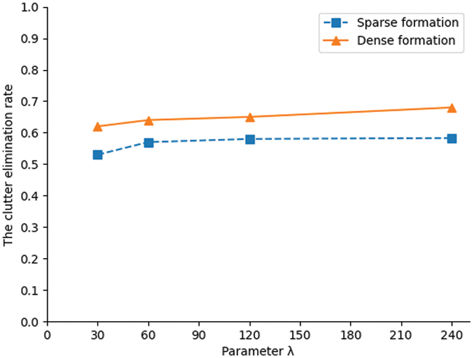
Figure 5: The clutter elimination rates

Fig. 5 shows the clutter elimination ability of RLCF. It can be seen from Fig. 5 that the clutter elimination rate in dense formation is greater than that in sparse formation. With the increase of the number of clutter, the clutter elimination rate also increases slowly, but it is basically stable at about 2/3. Theoretically, the measurements eliminated by clutter filtering are the ones that do not fall into the wave gates and are impossible to start the new tracks.

The farther the clutter measurements are from the target tracks, the less likely they fall into the wave gates and the more likely are eliminated. The experimental results also accord with the theory. The track wave gates coverage in dense formation is less than that in sparse formation. Therefore, the measurements outside the wave gate in dense formation are more than that in sparse formation. Therefore, the clutter elimination rate in dense formation is higher than that in sparse formation. Clutter elimination results are shown in Figs. 6 and 7, we can see that RLCF can remove clutter while retaining the real trace points.

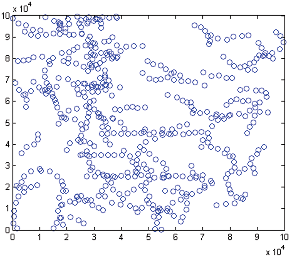
Figure 6: Clutter elimination results in sparse formation

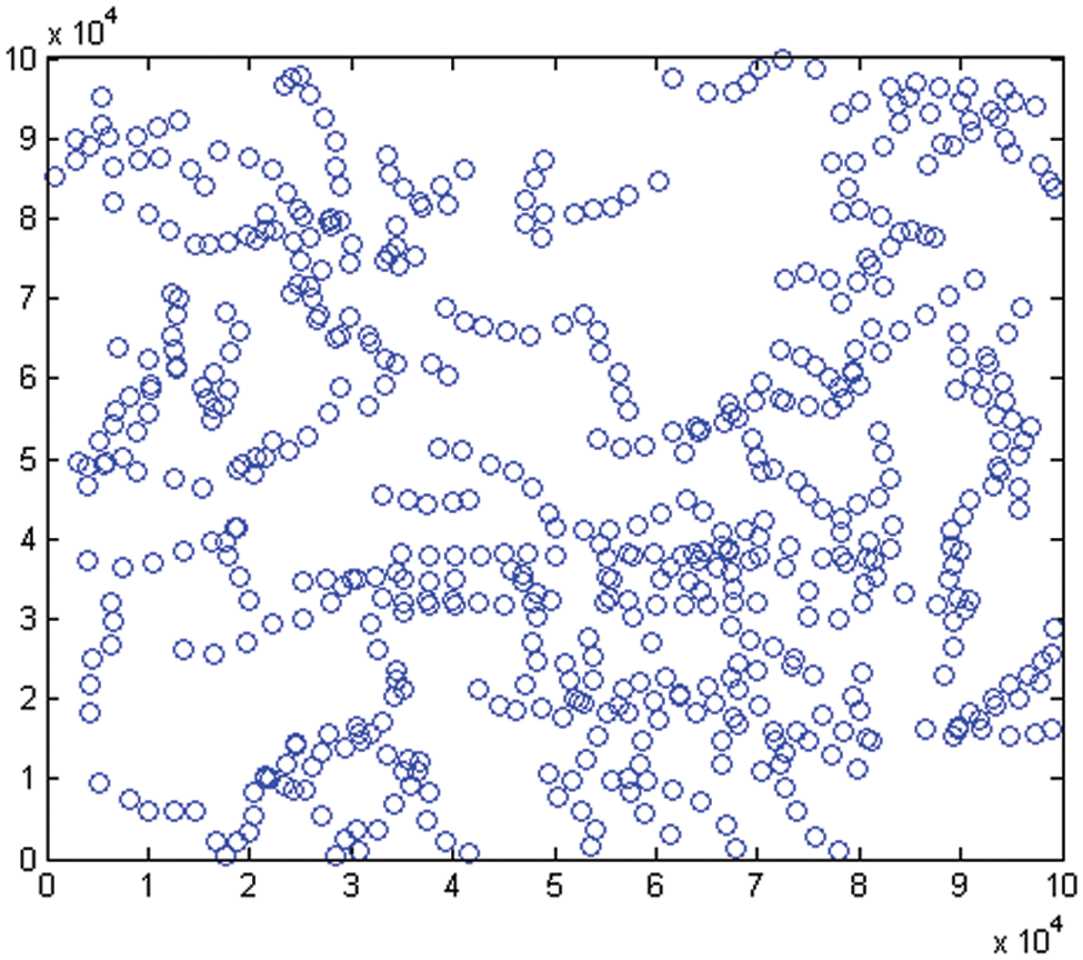
Figure 7: Clutter elimination results in dense formation

4.3 The Experiment for RLHTTI

The purpose of the experiment is to verify the performance of the relaxed logic-based Hough transform track initiation algorithm (RLHTTI), which is FSHTTI combined with RLCF. An environment with high false alarm and weak clutter is obtained by RLCF. The purpose of FSHTTI is to initiate the tracks accurately in such an environment. In order to more clearly show the performance of RLHTTI, this paper simulates two classical track initiation algorithms: modified logic track initiation algorithm (MLTI) and modified Hough transform track initiation algorithm (MHTTI). To evaluate the effect of RLHTTI, this paper sets up two groups of experiments and carries out 50 Monte Carlo simulations for each group of experiments.

The success rate of track initiation is the ratio of the number of correct tracks successfully initiated by the algorithm to the total number of real tracks in the experiment.

Pf3=∑i=1MCNis1MC∗Nreal(32)

where Pf3 is the success rate of track initiation. Nis1 is the number of correct tracks successfully initiated in the ith experiment. Nreal is the number of the targets.

False track occupancy rate is the ratio of the number of false tracks initiated (in the confirmed tracks) to the total number of target tracks established in the experiment.

Pf4=∑i=1MCNis2∑i=1MCNi(33)

where Pf4 is false track occupancy rate. Nis2 is the number of false tracks initiated in the ith experiment. Ni is the number of correct tracks successfully initiated in the ith experiment.

Firstly, the results of three track initiation algorithms are shown. When λ=240, the results of RLHTTI are shown in Figs. 8 and 9, the results of MLTI are shown in Figs. 10 and 11, and the results of MHTTI are shown in Figs. 12 and 13. It can be seen from the results that RLHTTI can accurately initiate the multi-target tracks in heavy clutter. Compared with MLTI and MHTTI, RLHTTI is hardly affected by the formation state.

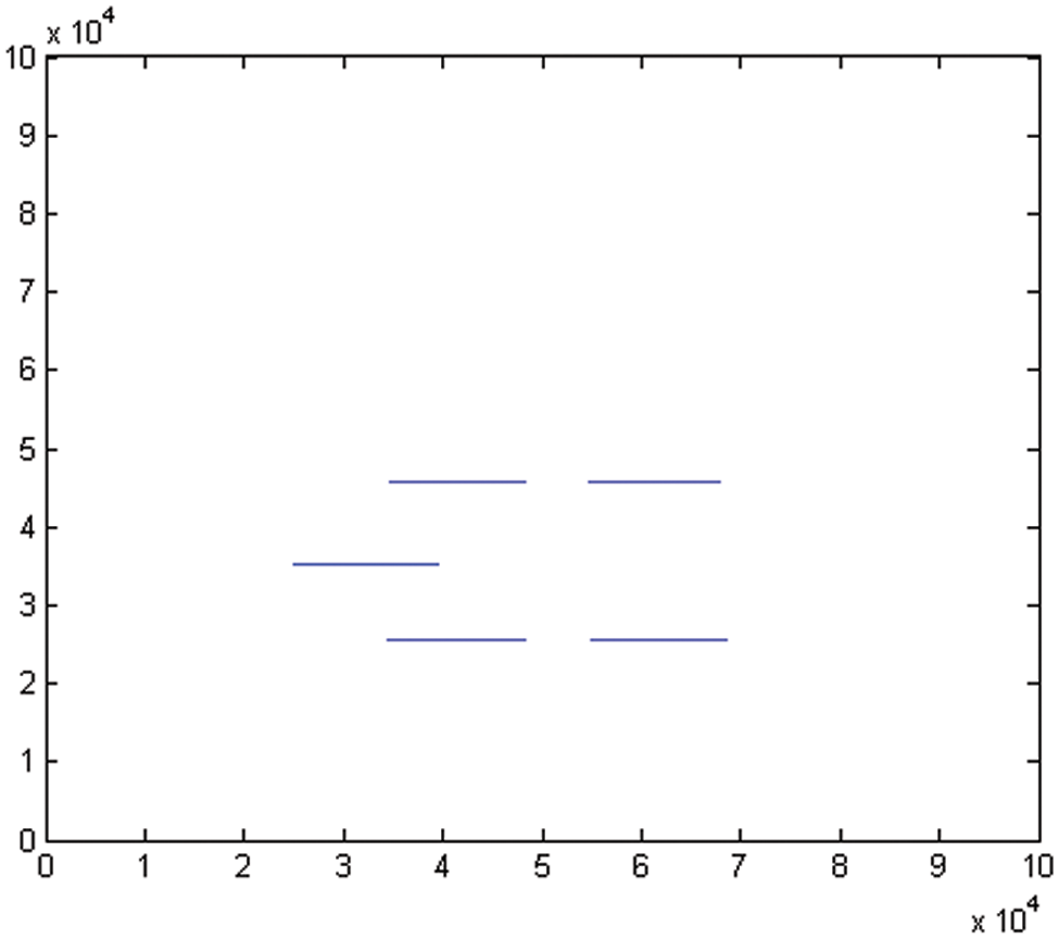
Figure 8: TI results of RLHTTI in sparse formation

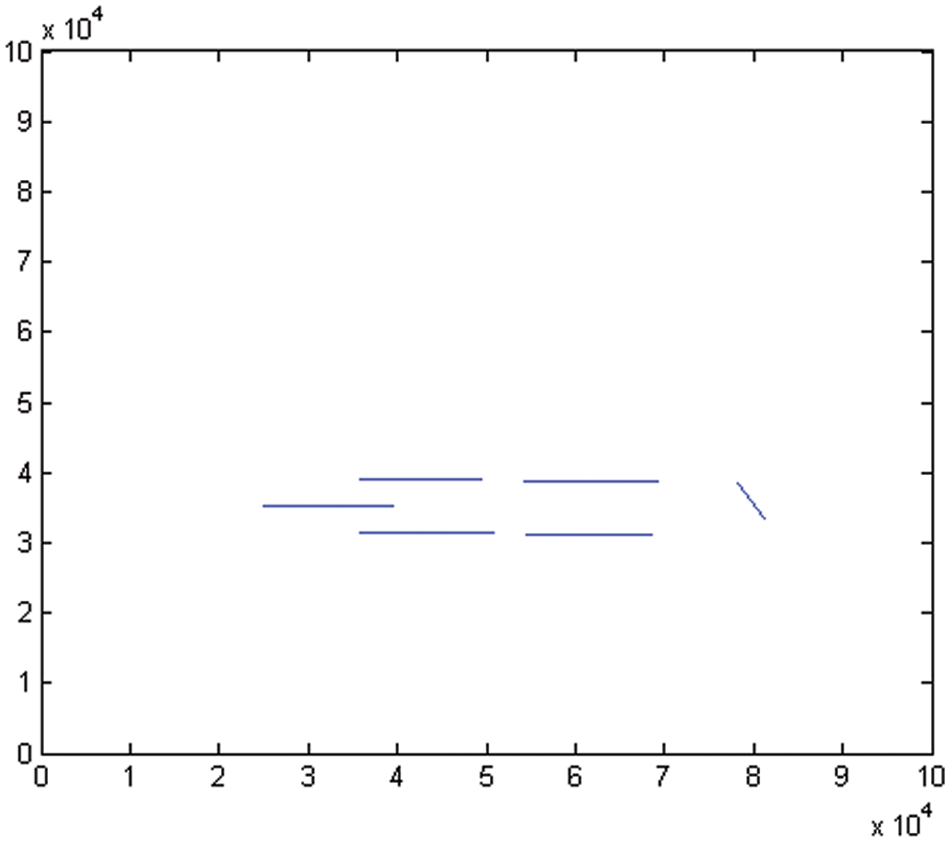
Figure 9: TI results of RLHTTI in dense formation

Figure 10: TI results of MLTI in sparse formation

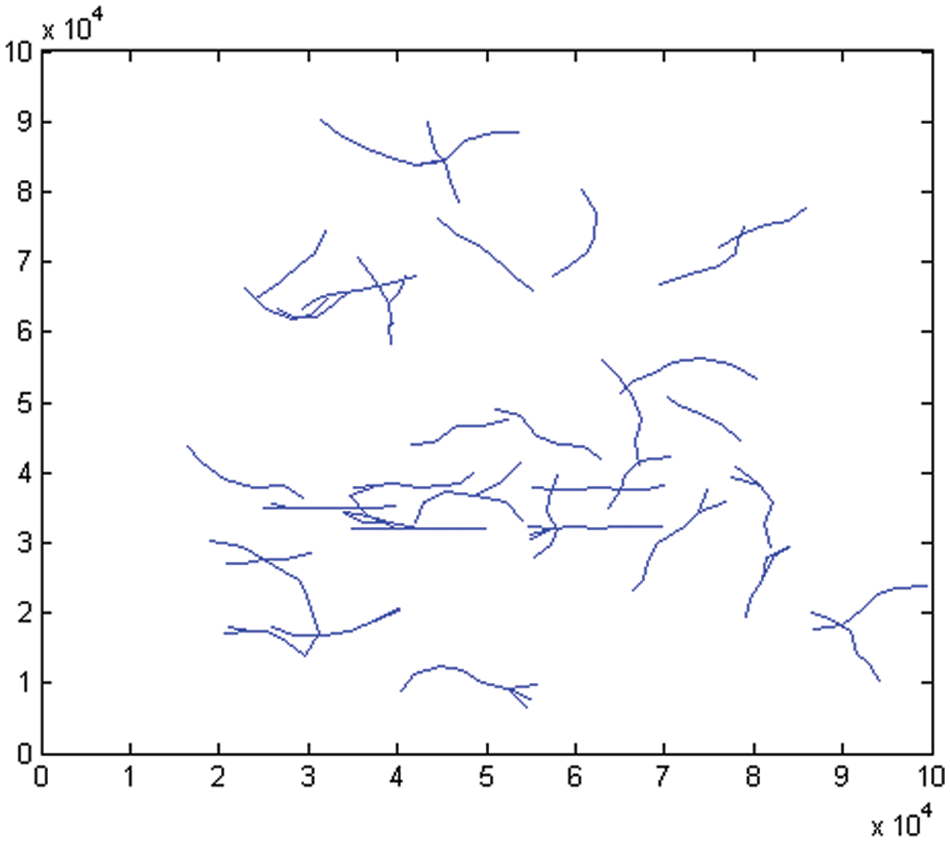
Figure 11: TI results of MLTI in dense formation

Figure 12: TI results of MHTTI in sparse formation

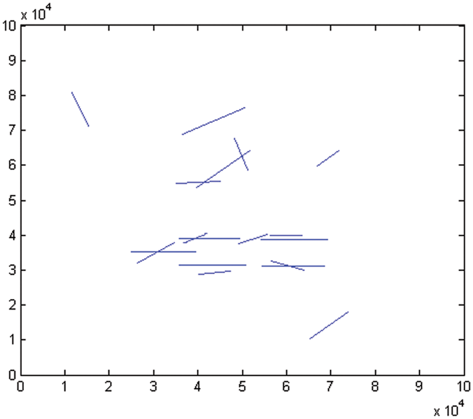
Figure 13: TI results of MHTTI in dense formation

The comparison results of the track initiation success rate and false track occupancy rate acquired by the three algorithms with 50 Monte Carlo experiments are shown in Figs. 14–17.

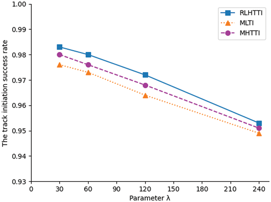
Figure 14: The comparison of the track initiation success rate in sparse formation

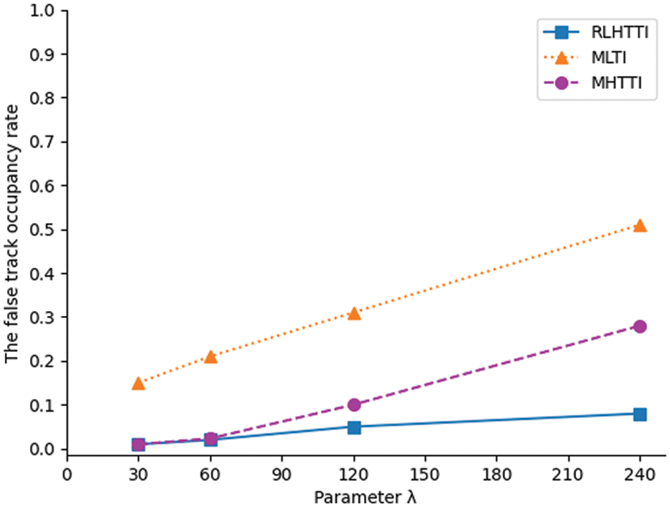
Figure 15: The comparison of the false track occupancy rate in sparse formation

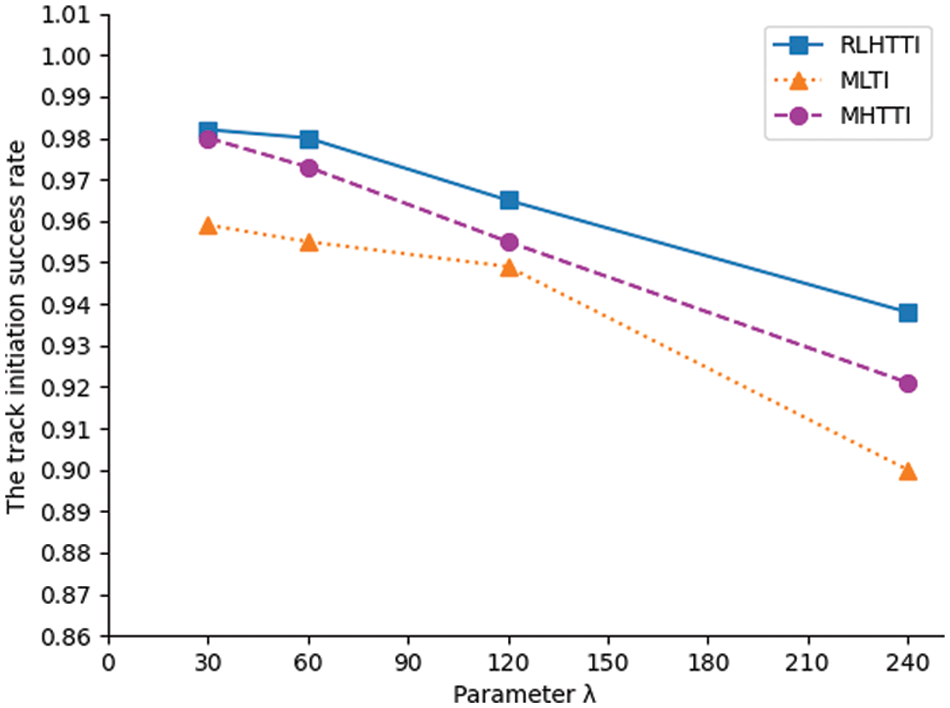
Figure 16: The comparison of the track initiation success rate in dense formation

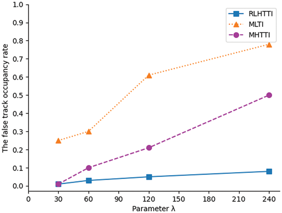
Figure 17: The comparison of the false track occupancy rate in dense formation

It can be seen from Figs. 14–17 that MLTI and MHTTI are greatly affected by the formation state. However, no matter what the formation state is, the track initiation success rate of RLHTTI is higher than MLTI and MHTTI, and the false track occupancy rate is much lower than MLTI and MHTTI. These achievements are due to the clutter filtering process and the superposition matrix constructed by fuzzy Hough transform, which effectively eliminates clutter measurements, weakens transformation error, and greatly improves the accuracy of the algorithm. In addition, because the algorithm modifies the matrix superposition rule of sequence Hough transform, the algorithm can accurately initiate the tracks in different formation states. The comparsions of the average initiation time are shown in Tabs. 3 and 4.

RLHTTI expands the wave gate, reduces the calculation of splitting extrapolation, eliminates clutter and reduces the number of measurements involved in Hough transform, but RLHTTI has no advantage over MLTI and MHTTI in the initiation time. Even in the weak clutter, the efficiency of RLHTTI is lower than that of MLTI and MHTTI. This is because RLHTTI is a serial combination of relaxed logic and sequential Hough transform, and the construction of fuzzy superposition matrix requires additional calculation. However, RLHTTI is less affected by the number of clutter and target formation states and has better universality and stability. With the same time consumption, RLHTTI can more effectively suppress false tracks and obtain more accurate track initiation in heavy clutter. In short, compared with MLTI and MHTTI, RLHTTI has higher performance in track initiation.

5  Conclusions

The paper focuses on the key problems of track initiation in the heavy clutter, and gives the corresponding solutions. The raw measurements are filtered by using the relaxed logic method. And the tracks are initiated by fuzzy sequential Hough transform. Through comparative experiments, the accuracy of track initiation and the suppression ability of false tracks of this algorithm are verified. The algorithm has performed well in the multi-target environment. However, due to the influence of heavy clutter, the algorithm has the phenomenon of missing alarm. To obtain a higher success rate of track initiation, reducing the missing alarm of track initiation is our future work.

Funding Statement: This work is supported in part by the Fundamental Research Funds for the Central Universities, Jilin University under Grant No. 93K172021K04.

Conflicts of Interest: The authors declare that they have no conflicts of interest to report regarding the present study.

References

 1.  H. Masood, A. Zafar, M. U. Ali, M. A. Khan, S. Ahmed et al., “Recognition and tracking of objects in a clustered remote scene environment,” Computers, Materials & Continua, vol. 70, no. 1, pp. 1699–1719, 2022. [Google Scholar]

 2.  H. Sun, M. Luo, X. Wu and X. Xie, “Labelled GM-CBMEMBER filter with adaptive track initiation,” The Journal of Engineering, vol. 2019, no. 19, pp. 6028–6033, 2019. [Google Scholar]

 3.  D. Li, Y. Lin and Y. Zhang, “A track initiation method for the underwater target tracking environment,” China Ocean Engineering, vol. 32, no. 2, pp. 206–215, 2016. [Google Scholar]

 4.  W. Wu, H. Sun, Y. Cai, S. Jiang and J. Xiong, “Tracking multiple maneuvering targets hidden in the DBZ based on the MM-GLMB filter,” IEEE Transactions on Signal Processing, vol. 68, pp. 2912–2924, 2020. [Google Scholar]

 5.  Y. Zhang, S. Yang, H. Li and H. Mu, “A novel multi-target track initiation method based on convolution neural network,” in Proc. RSIP, Shanghai, China, pp. 1–5, 2017. [Google Scholar]

 6.  F. Yang, Y. Luo, Q. Li and Y. Yin, “A hypothesis-optimized RANSAC algorithm for track initiation,” in Proc. 23rd FUSION, South Africa, pp. 1–6, 2020. [Google Scholar]

 7.  X. R. Zhang, X. Sun, X. M. Sun, W. Sun and S. K. Jha, “Robust reversible audio watermarking scheme for telemedicine and privacy protection,” Computers, Materials & Continua, vol. 71, no. 2, pp. 3035–3050, 2022. [Google Scholar]

 8.  C. Liu, Q. Wang, S. Yang and S. Li, “Track initiation with orthogonal EDS statistics,” in Proc. CAC, Hangzhou, China, pp. 1321–1327, 2019. [Google Scholar]

 9.  S. W. Kim, H. D. Cho and T. I. Kwon, “A study on the improvement of robust automatic initiated tracking on narrowband target,” The Journal of the Acoustical Society of Korea, vol. 39, no. 6, pp. 549–558, 2020. [Google Scholar]

10. L. Guo, J. Lan and X. R. Li, “Track initiation in the presence of multipath effect and reflecting point uncertainties,” in Proc. 22th FUSION, Canada, pp. 1–8, 2019. [Google Scholar]

11. J. A. Gaebler, P. Axelrad and P. W. Schumacher Jr, “CubeSat cluster deployment track initiation via a radar admissible region birth model,” Journal of Guidance, Control, and Dynamics, vol. 43, no. 10, pp. 1927–1934, 2020. [Google Scholar]

12. M. Luo, X. Wu, H. Sun, X. Xin and C. Wu, “A labeled SMC-Cbmember filter with adaptive track initiation,” IOP Conference Series: Materials Science and Engineering, vol. 452, no. 4, pp. 042203, 2018. [Google Scholar]

13. S. Liu, H. Li, Y. Zhang, B. Zou and J. Zhao, “Random forest-based track initiation method,” The Journal of Engineering, vol. 19, pp. 6175–6179, 2019. [Google Scholar]

14. G. Lee, N. Kwak, J. Kwon, E. Yang and K. Kim, “Track initiation algorithm based on weighted score for TWS radar tracking,” Journal of the Korea Institute of Military Science and Technology, vol. 22, no. 1, pp. 1–10, 2019. [Google Scholar]

15. Q. Jiang, R. Wang, C. Zhou, T. R. Zhang and C. Hu, “Modified Bayesian group target track initiation algorithm based on algebraic graph theory,” Journal of Electronics & Information Technology, vol. 43, no. 3, pp. 531–538, 2021. [Google Scholar]

16. J. Baek, J. Lee, H. Shim, S. Im and Y. Han, “Target tracking initiation for multi-static multi-frequency PCL system,” IEEE Transactions on Vehicular Technology, vol. 69, no. 10, pp. 10558–10568, 2020. [Google Scholar]

17. E. F. Wilthil, E. Brekke and O. B. Asplin, “Track initiation for maritime radar tracking with and without prior information,” in Proc. 21st FUSION, United Kingdom, pp. 1–8, 2018. [Google Scholar]

18. Z. Liu, X. Zhu and B. Huang, “Track initiation technique and its application in PHD filter,” in Proc. 14th ICSP, Beijing, China, pp. 822–826, 2018. [Google Scholar]

19. A. Hunde and B. Ayalew, “Linear multi-target integrated probabilistic data association filter with automatic track management for autonomous vehicles,” in Proc. DSCC, Atlanta, Georgia, USA51906, pp. V002T15A001, 2018. [Google Scholar]

20. I. Vaughan, L. Clarkson and J. L. Williams, “Tracker operating characteristic for integrated probabilistic data association,” in Proc. RADAR, Australia, China, pp. 27–31, 2018. [Google Scholar]

21. C. Han, B. Sun and J. W. Li, “A new track initiation algorithm based on hierarchical clustering and correlation coefficient,” in Proc. 5th ICSIP, Nanjing, China, pp. 1071–1074, 2020. [Google Scholar]

22. Z. Wang, M. Li, Y. Lu, H. Chen and W. Yan, “Efficient TR-TBD algorithm for slow-moving weak multi-targets in heavy clutter environment,” IET Signal Process, vol. 11, no. 4, pp. 422–428, 2017. [Google Scholar]

23. X. R. Zhang, W. F. Zhang, W. Sun, X. M. Sun and S. K. Jha, “A robust 3-D medical watermarking based on wavelet transform for data protection,” Computer Systems Science & Engineering, vol. 41, no. 3, pp. 1043–1056, 2022. [Google Scholar]

24. Y. Ren, F. Zhu, K. S. Pradip, T. Wang, J. Wang et al., “Data query mechanism based on hash computing power of blockchain in internet of things,” Sensors, vol. 20, no. 1, pp. 1–22, 2020. [Google Scholar]

25. S. Ebrahimi, G. Sarbishaei and G. A. Hodtani, “Off-grid direction of arrival estimation in the presence of measurement noise and heavy cluttered environment,” Signal Image Video Process, vol. 15, no. 4, pp. 695–703, 2021. [Google Scholar]

26. L. Wu, J. Mao and W. Bai, “Radar small/mini target detection technology in strong clutter environment,” The Journal of Engineering, vol. 20, no. 2019, pp. 7130–7133, 2019. [Google Scholar]

27. Y. Zhang, A. Liu, C. Liu, B. Ai and X. Zhang, “A track initiation algorithm using residual threshold for shore-based radar in heavy clutter environments,” Journal of Marine Science and Engineering, vol. 8, no. 8, pp. 614, 2020. [Google Scholar]

28. Z. Q. Jin, G. L. Liu, Y. Lu, J. Q. Zhang and W. Zhao, “Multi-platform track initiation method in dense clutter environment,” in Proc. ICCAIS, Chengdu, China, pp. 1–5, 2019. [Google Scholar]

29. H. H. Sönmez, K. Turgut and A. K. Hocaoğlu, “Improving track initiation performance by track validation algorithms for multi-target tracking in heavy clutter,” in Proc. 25th SIU, Antalya, Turkey, pp. 1–4, 2017. [Google Scholar]

30. G. Lee, S. Lee, K. Kim and N. Kwak, “Probabilistic track initiation algorithm using radar velocity information in heavy clutter environments,” in Proc. 15th EuRAD, Spain, pp. 277–280, 2018. [Google Scholar]

31. Y. Ren, Y. Leng, J. Qi, S. K. Pradip, J. Wang et al., “Multiple cloud storage mechanism based on blockchain in smart homes,” Future Generation Computer Systems, vol. 115, no. 2, pp. 304–313, 2021. [Google Scholar]

This work is licensed under a Creative Commons Attribution 4.0 International License, which permits unrestricted use, distribution, and reproduction in any medium, provided the original work is properly cited.