Computers, Materials & Continua DOI:10.32604/cmc.2022.027874
Article

Enhancing Collaborative and Geometric Multi-Kernel Learning Using Deep Neural Network

Bareera Zafar1, Syed Abbas Zilqurnain Naqvi1, Muhammad Ahsan1, Allah Ditta2,*, Ummul Baneen1 and Muhammad Adnan Khan3,4

1Department of Mechatronics and Control Engineering, University of Engineering and Technology, Lahore, 54890, Pakistan
2Department of Information Sciences, Division of Science and Technology, University of Education, Lahore, 54000, Pakistan
3Riphah School of Computing & Innovation, Faculty of Computing, Riphah International University, Lahore Campus, Lahore, 54000, Pakistan
4Department Software, Gachon University, Seongnam, 13120, Korea
*Corresponding Author: Allah Ditta. Email: allahditta@ue.edu.pk
Received: 27 January 2022; Accepted: 08 March 2022

Abstract: This research proposes a method called enhanced collaborative and geometric multi-kernel learning (E-CGMKL) that can enhance the CGMKL algorithm which deals with multi-class classification problems with non-linear data distributions. CGMKL combines multiple kernel learning with softmax function using the framework of multi empirical kernel learning (MEKL) in which empirical kernel mapping (EKM) provides explicit feature construction in the high dimensional kernel space. CGMKL ensures the consistent output of samples across kernel spaces and minimizes the within-class distance to highlight geometric features of multiple classes. However, the kernels constructed by CGMKL do not have any explicit relationship among them and try to construct high dimensional feature representations independently from each other. This could be disadvantageous for learning on datasets with complex hidden structures. To overcome this limitation, E-CGMKL constructs kernel spaces from hidden layers of trained deep neural networks (DNN). Due to the nature of the DNN architecture, these kernel spaces not only provide multiple feature representations but also inherit the compositional hierarchy of the hidden layers, which might be beneficial for enhancing the predictive performance of the CGMKL algorithm on complex data with natural hierarchical structures, for example, image data. Furthermore, our proposed scheme handles image data by constructing kernel spaces from a convolutional neural network (CNN). Considering the effectiveness of CNN architecture on image data, these kernel spaces provide a major advantage over the CGMKL algorithm which does not exploit the CNN architecture for constructing kernel spaces from image data. Additionally, outputs of hidden layers directly provide features for kernel spaces and unlike CGMKL, do not require an approximate MEKL framework. E-CGMKL combines the consistency and geometry preserving aspects of CGMKL with the compositional hierarchy of kernel spaces extracted from DNN hidden layers to enhance the predictive performance of CGMKL significantly. The experimental results on various data sets demonstrate the superior performance of the E-CGMKL algorithm compared to other competing methods including the benchmark CGMKL.

Keywords: CGMKL; multi-class classification; deep neural network; multiple-kernel learning; hierarchical kernel spaces

1  Introduction

Machine learning has become necessary nowadays in every sector of life. Machine learning methodologies for binary classification like decision trees, Support Vector Machines, K-nearest neighbor, neural network, and Naïve Bayes can be extended for multi-class classification [1]. The most common traditional techniques used for multiclass classification are one-vs.-one (OVO) and one-vs.-all (OVA). In OVA a single classifier is designed per class i-e if there are K classes then K classifiers are constructed. When data is given as input to the classifiers then the classifier that belongs to a particular class gives the highest probability value for that class [2]. But an imbalance problem exists in OVA because single class samples are much less as compared to the number of samples in the remaining classes [3]. OVO approach divides the problem into n(n+1)2 binary classifiers or sub-problems. The outputs of these base classifiers are combined to get the final output [2]. The results show that OVO performance is better as compared to OVA [4]. But the OVO method is encountered by non-competence problems [5]. In both of the methods, OVO and OVA, there is an issue of computational inefficiency due to the formation of several binary classifiers. To overcome the limitations mentioned above, the softmax function is used which requires much easier parameter learning strategies and optimizes a single log-likelihood function during the training phase. The outcome of a softmax function is a monomial probability distribution on k number of possible classes. The class with the highest probability is the predicted class [6]. For a given test sample, softmax directly outputs the probability of that sample belonging to a particular class, hence avoiding the need to develop multiple binary classifiers.

Although the softmax function deals well with multi-class classification problems when the data distributions have linear decision boundaries, it encounters performance degradation on nonlinear data sets. This problem is addressed by employing kernel methods that map the original data points to higher dimensional feature space to make the classification task easier. Some kernel methods construct implicit feature representations in the higher dimensional space through the use of kernel function, but this approach does not apply to softmax function. To combine kernel methods with softmax function, empirical kernel mapping (EKM) is used [7]. EKM maps each sample x into an explicit feature vector φe(x) in the high dimensional kernel space. Once φe(x) is computed it can be easily inserted into the softmax function [8]. Introduces the collaborative and geometric multi-kernel learning (CGMKL) algorithm which effectively incorporates the multiple empirical kernel learning (MEKL) framework into the softmax function. CGMKL enhances the expression of sample data through empirical feature space φe and enriches the classification ability of the softmax function. Additionally, CGMKL ensures collaborative working of softmax function among different kernel spaces and improves classification of all kernel spaces by controlling output trends of input samples. To accomplish these tasks, CGMKL employs two regularization terms: RTUnand RTSn. The term RTUn helps softmax function to collaboratively work in different kernel spaces. This term harmonizes the information between different kernel spaces and provides consistent outputs of samples in them. The term RTSn reduces the within-class distance and improves the classification capability of all kernel spaces. However, the kernels constructed by CGMKL do not have any explicit relationship among them, and hence try to construct high dimensional feature representations independently from each other. This could be disadvantageous for learning on datasets with complex hidden structures. To address this issue, one possible solution is to construct kernel spaces from hidden layers of trained deep neural networks (DNN). Due to the nature of the DNN architecture, these kernel spaces not only provide multiple feature representations but also inherit the compositional hierarchy of the hidden layers which might be beneficial for improving the predictive performance of the CGMKL algorithm on complex data.

Deep learning is a subset of machine learning that employs deep neural network architectures in which multiple hidden layers help to learn a more abstract representation of data as we move progressively from the shallow to the deeper layers. Deep learning methodologies surpass traditional machine learning algorithms especially when the data becomes huge or problems become complex, for example, image classification, natural language processing (NLP), and speech recognition problems [9]. Usually, in deep neural networks, only the last hidden layer is used to get the final output and intermediate representations of hidden layers are used for preparing a more abstract representation of the output layer. In [10] KerNET method is proposed and applied on two renowned architectures i-e multi-layer perceptron (MLP) and convolutional neural network (CNN). Motivated from [10] our paper likewise exploits the information of intermediate representations extracted from the hidden layers of a trained DNN. The output of the nth hidden layer “ φn” is used as a feature vector to make a base kernel Kn(i,j)=φn(xi).φn(xj). The multiple kernel spaces constructed from these hidden layers inherit the compositional hierarchy of the hidden layers. This hierarchical structure might help improve the predictive performance of the classification algorithm on data sets with complex hidden structures.

This paper proposes an enhanced collaborative and geometric multi-kernel learning (E-CGMKL) algorithm that can enhance the CGMKL algorithm, and deal with complex multi-class classification problems with non-linear data sets. Below we provide a list that highlights the advantages of our proposed method over CGMKL:

(a)  The kernels constructed by CGMKL do not have any explicit relationship among them and try to construct high dimensional feature representations independently from each other. This could be disadvantageous for learning on datasets with complex hidden structures. To overcome this limitation, E-CGMKL constructs kernel spaces from hidden layers of trained deep neural networks (DNN). Due to the nature of the DNN architecture, these kernel spaces not only provide multiple feature representations but also inherit the compositional hierarchy of the hidden layers, which might be beneficial for enhancing the predictive performance of the CGMKL algorithm on complex data with natural hierarchical structures, for example, image data.

(b)  Furthermore, our proposed scheme handles image data by constructing kernel spaces from a convolutional neural network (CNN). Considering the effectiveness of CNN architecture on image data, these kernel spaces provide a major advantage over the CGMKL algorithm which does not exploit the CNN architecture for constructing kernel spaces from image data.

(c)  Additionally, outputs of hidden layers directly provide features for kernel spaces and unlike CGMKL, do not require an approximate MEKL framework.

(d)  E-CGMKL combines the consistency and geometry preserving aspects of CGMKL with the compositional hierarchy of kernel spaces extracted from DNN hidden layers to enhance the predictive performance of CGMKL significantly.

This paper is organized as follows. Section 2 briefly describes existing work related to our research. Section 3 provides a detailed description of our proposed E-CGMKL algorithm. Section 4 presents and discusses experimental results. In the last section, conclusions are provided.

2  Related Work

Kernel method is a remarkable technique that converts nonlinear complex pattern data to a linear pattern in high dimensional reproducing hilbert kernel space (RHKS) [11].

2.1 Kernel Methods

Kernel Methods introduced in [12,13] such as support vector machines (SVM), Gaussian kernel, kernel principal component analysis (PCA), and kernel fisher discriminant analysis (KFDA) are well-established machine learning methods. These kernel methods use kernel functions K:XxX→R to implicitly map non-separable input data to a possibly high dimensional feature space by defining the inner product in that space: Kn(xi,xj)=φn(xi).φn(xj). Fig. 1 shows the Kernel function mapping of non-separable input data to separable high dimensional kernel space.

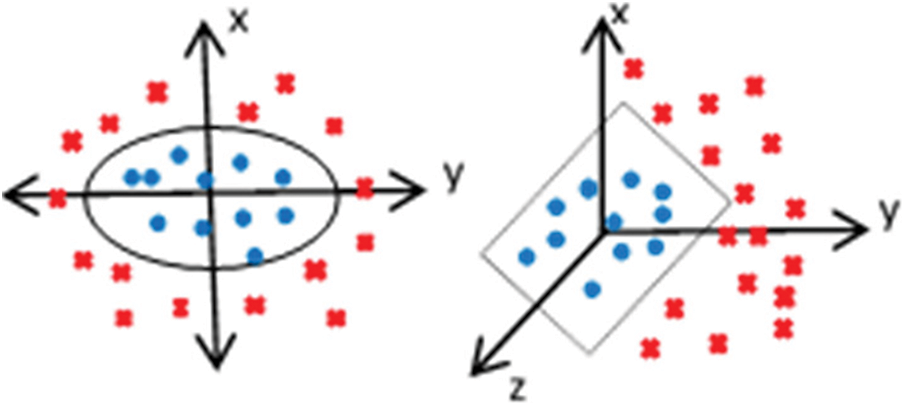
Figure 1: Graphical illustration of kernel mapping

2.2 Multiple Kernel Learning

The success of a kernel-based learning algorithm depends on appropriate kernel selection. Choice of the kernel is a fundamental problem of kernel methods. Various evaluation measures of kernel function for modal selection have been proposed such as kernel polarization [14], cross-validation, kernel alignment [15], and spectral analysis [16,17]. Yet, these mechanisms cannot guarantee an optimal selection of kernel functions for the good performance of kernel-based classifiers. To address this problem, a popular technique called multiple kernel learning (MKL) has attracted the attention of many researchers. MKL combines a set of base kernels constructed by using different kernel functions. The optimal combination of base kernels can automatically learn the importance of each feature [18–20]. Different algorithms have been proposed that try to improve the learning efficiency of MKL by exploiting various optimization techniques: Simple-MKL [21], Easy-MKL [22], and stochastic variance reduced gradient SVRG-MKL [23]. To improve the regular MKL, extended MKL techniques have been proposed e-g Localized MKL (LMKL), novel sample-wise alternating optimization for training LMKL [24]; Sample Adaptive MKL, adaptively switch base kernels corresponding to each sample [25]; Bayesian Maximum Margin MKL, improves the learning speed and generalization ability by defining a multiclass likelihood function that accounts for margin loss for kernelized classification [26]; and Multiple Empirical Kernel Learning (MEKL) which explicitly represents the samples by mapping input space to explicit feature space [27].

2.3 Deep Learning and Conventional Machine Learning

There are some traditional machine learning algorithms used for multi-class classification namely random forest, support vector machine (one vs. one) SVM (OVO), support vector machine (one vs. all) SVM (OVA), and BPNN. Random forest is an ensemble method introduced by Breiman in 2001 [28], it involves a group of tree-structured predictors in learning process. This approach is used in [29] for diabetes classification effectively. But this method consists of a lot of trees in learning which makes it computationally expensive and is also not known to perform well on image and audio data. SVM (OVO) and SVM (OVR) are the most common classification techniques in which SVM (OVO) divides the problem into n(n+1)2 binary classifiers and in SVM (OVA) single classifier is used per class. Reference [30] implements OVO and OVA approach to extract discriminative features and to predict multiclass motor imagery features respectively. Both of the methods encounter the issue of computational inefficiency because of the formation of several binary classifiers. Back propagation neural network (BPNN) is a supervised learning algorithm used for classification. In [31] BPNN algorithm is designed to predict the silicon oxide content during chemical analysis estimated according to rock main oxide. In BPNN only the last layer representation gives the classification result but intermediate representations can be used for the main classification task.

In deep kernel learning, there are three current research directions. The first one is to form a synergy model in which a front-end deep module is used and a kernel machine is used at the back-end. This type of work has been done in [32] which presented a hybrid system in which a CNN identifies generic objects, and the features learned through CNN are used in training Gaussian-kernel SVM. This type of work can also be found in [33]. In the second direction, the kernel method is fitted in deep architectures. Reference [34] introduces a convolutional kernel network (CKN) which fills the gap between kernels and neural network literature. Kernels in CKN produce representations of the images in a sequence built-in multilayer fashion and these layers are named image feature maps. Similar work has been done by Reza et al. in [35]. The third direction is to combine the idea of deep kernel learning and optimization. Reference [36] introduces scalable deep learning which combines the structural properties of deep neural networks with the nonparametric flexibility of kernel methods, by presenting scalable probabilistic gaussian processes. Semi-supervised deep kernel learning [37] is the extension of this work [11].

In the context of complex feature learning using deep nets [38] recently proposed TBE-net algorithm. TBE-Net provides complex feature learning and leads to more integral diverse vehicle features. Recently [39] proposed RSOD algorithm for small object detection which smartly exploits the feature maps generated by the shallow and deep layers as well as employs an attention mechanism to improve the detection accuracy. In [10] Lauriola et al. proposed a deep learning framework named as KerNet. This framework combines the hidden layer representations optimally through the multi-kernel learning (MKL) framework. This combination improves the quality and performance of the final representation. Each hidden layer output has a feature vector φ(x) corresponding to each input sample x which is used to build the base kernels Kn(xi,xj)=φn(xi).φn(xj). These base kernels are then combined using the MKL framework i-e K=∑l⁡μlKl. Fig. 2 illustrates this process. In [8] Wang et al. introduce the CGMKL algorithm for multiclass classification which ensures consistent outputs of samples across multiple kernel spaces and minimizes the within-class distance to highlight the clustering of different classes but it does not use structurally related kernel spaces. In this paper, a hybrid mechanism is proposed which combines the kerNET framework with CGMKL. We exploit the intermediate representations extracted from hidden layers of trained DNN to construct multiple kernel spaces which inherit the compositional hierarchy of the hidden layers. These kernel spaces are then used in the CGMKL method to enhance its predictive performance.

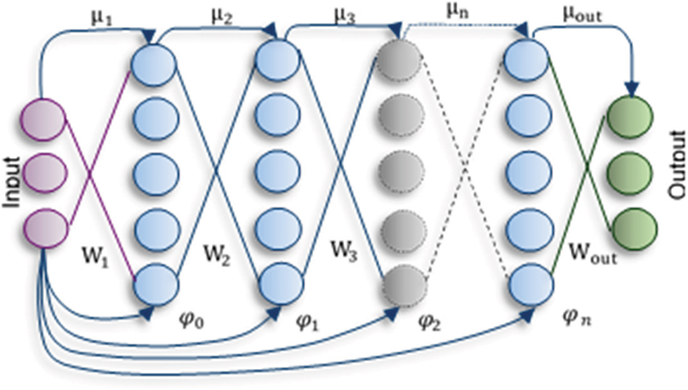
Figure 2: Neural network architecture showing the inner representation of input samples at nth hidden layer φn and arranged sequence of nonlinear transformations  μ1,…,μn

3  Methodology

Deep neural network architecture output depends on the compositional sequence of non-linear mapping that conveys progressively complex representations of input data. In this paper, we are using intermediate representations extracted from a hidden layer of DNN. The mathematical model of these intermediate representations is described by the function φn(x) which is the composite function given by:

φn(x)=μnoμn−1o…μ1(x)(1)

where μn(x)=g(Wn(x)+b) represents a nonlinear transformation from n−1 to nth hidden layers and φ0=x is the input sample as illustrated in Fig. 2.

3.1 Multiple Kernel Spaces Extracted from DNN

E-CGMKL algorithm can be applied to any DNN architecture. There are two main architectures used in this work namely MLP and CNN. In MLP architecture the neural network weights are fully trained using Keras and Tensor-flow libraries by selecting the best hyperparameters. Afterward, the output of the nth hidden layer of the trained network is used to make the nth base kernel Kn(xi,xj)=φn(xi).φn(xj). The kernel spaces constructed from these hidden layers inherit the compositional hierarchy of the hidden layers and hence, enhance the ability of the softmax function to classify non-separable datasets with complex hidden structures. In the case of CNN, the output of the hidden layer is not in the form of a single vector as in the case of MLP architecture, instead, it is in the form of a tensor whose dimension depends on the pixels of the input image times the number of filters used in the hidden layer. So, the output of the hidden layer is flattened before using it as a feature vector. CNN architecture also has different types of layers e.g., convolutions, pooling, dropout, and dense from which only the representations of convolution and dense layers have been used. The notation φn(x) used for CNN is depicted in Fig. 3.

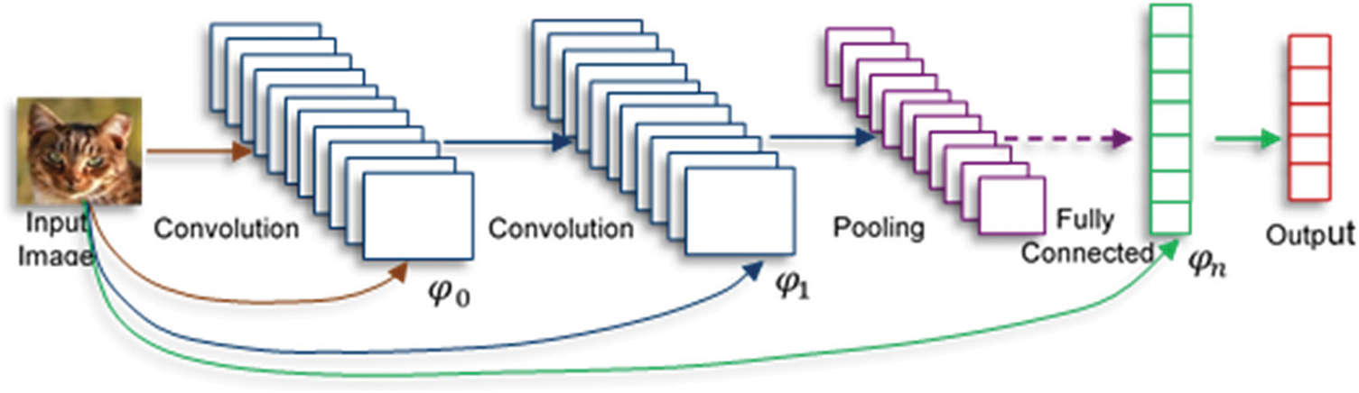
Figure 3: Convolutional neural network (CNN) architecture is composed of convolution, pooling, and fully connected layers. As the figure illustrates the intermediate representation φnis defined by the output convolution and fully connected layer

3.2 E-CGMKL Algorithm

A brief mathematical description of the CGMKL algorithm [8] is given below. The overall loss function of the CGMKL algorithm is given as follows.

L=∑n=0l⁡[Lstm(fn)+δRTSn]+σRTUn(2)

In Eq. (2) Lstm(fn) is the loss of softmax function written as below:

Lstm(fn)=∑i=1N⁡log⁡(exp⁡(xinWn)yiTexp⁡(xinWn)1⇀)(3)

If there are Nnumber of samples in training set then N samples are defined as xin=[φne(x),1] which represents the feature vector in nthkernel space corresponding to ith training sample and Wn is the weight matrix of nth kernel space which is learned during parameter learning. If R is the number of neuron in DNN hidden layer and C is the number of classes then the dimension of Wn matrix is RXC In Eq. (2) RTUn is the regularization term that helps softmax function to collaboratively work in different kernel spaces. This term harmonizes the information between different kernel spaces and provides consistent outputs of samples in them and σ is the parameter that controls the importance of RTUn. The detailed term is given as:

RTUn=12N∑n=0l⁡tr((XinWn−1l∑j=1l⁡XijWj)(XinWn−1l+1∑j=1l⁡XijWj)T) (4)

In Eq. (4) Xin represents matrix form of intermediate representation of each sample xin=[φne(x),1]. Dimension of Xin is NX(R+1)RTSn is another regularization term in Eq. (2). To exhibit a geometric feature of classification results this term reduces the within-class distance and δis the parameter that controls the importance of RTSn. In this term, Sn is the scatter matrix in lth kernel space. The formula of RTSn is given below:

RTSn=12Ntr(SnWnWnTSnT)(5)

In Eq. (5) Sn for each kernel space is calculated by taking the mean of intermediate representation of samples in each class in φn(x). Next the class mean of intermediate representation is subtracted from the corresponding intermediated representation of that class. Dimension of Sn is RXR. Derivative of loss function of Eq. (2) with respect to Wn is given as:

∂L∂Wn=∑i=1N xinT(log(exp(xinWn)exp(xinWn)1⇀)−yiT)+δNSnTSnWn+σN(l−1lXnTXnWn−1lXnT∑j=1,j≠nlXjWj)(6)

For parameter learning, RMSProp is used as an optimization method. To reach global minima faster, RMSprop uses the memory matrix δ∂Wm to store the previous gradient.

δ∂Wnnew=βδ∂Wn+(1−β)(∂L∂Wn)2(7)

Finally, RMSProp updates the weight equation as:

Wnnew=Wn−α(1δ∂Wnnew+ϵ)∂L∂Wn(8)

In the above Eq. (7) β is the RMSProp parameter and in Eq. (8) αis the learning rate. A slight modification in the prediction step of the CGMKL algorithm is also proposed. Unlike CGMKL the following equation is used to predict the label for the test sample.

F(x)=∑n=1l⁡μlxnWn(9)

where ‘ μl’ are the weights given by the EASYMKL algorithm (multiple kernel learning algorithm). These weights measure the importance of each kernel and provide an optimal combination of kernel spaces for test sample prediction.

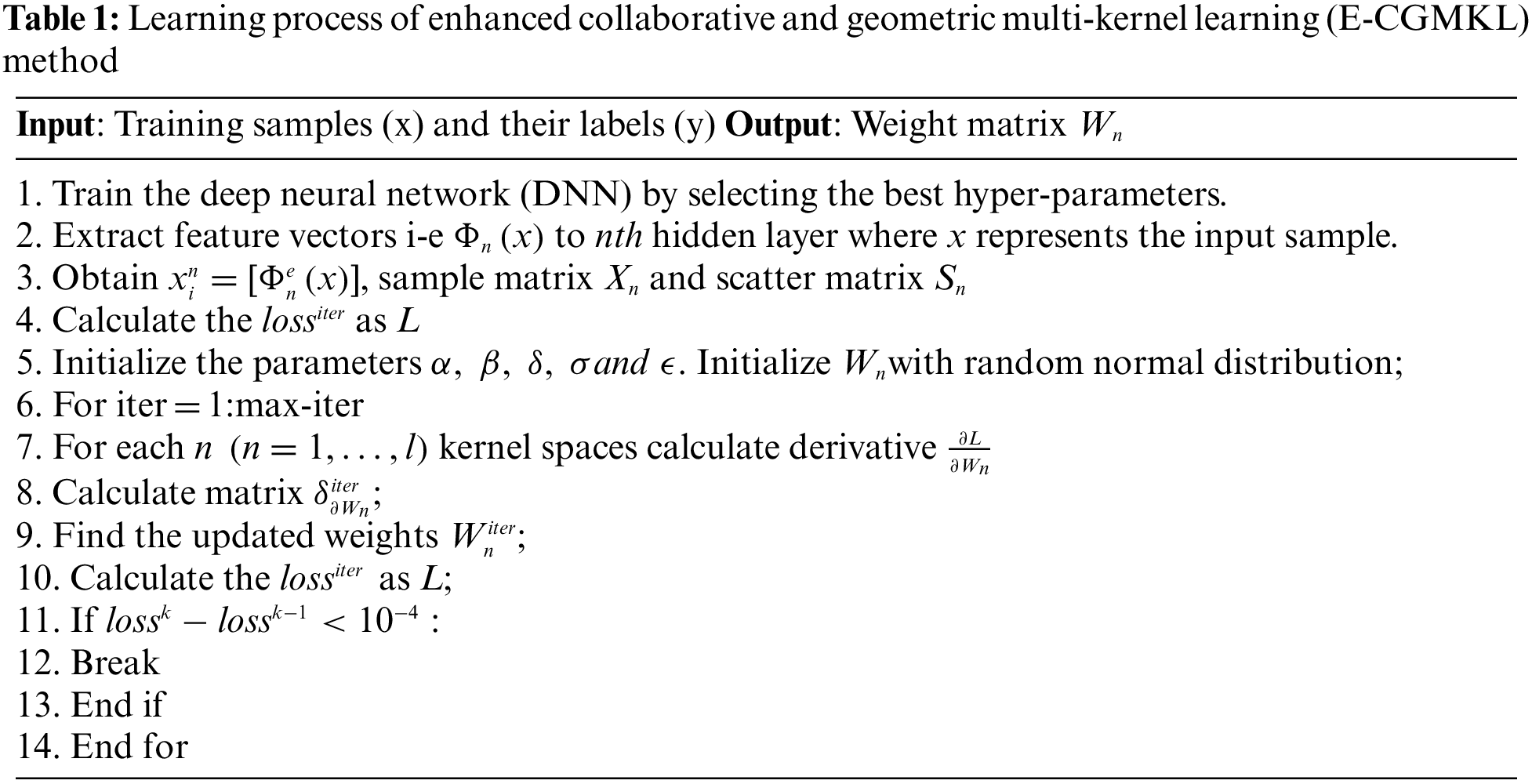
3.3 Training the E-CGMKL Algorithm

The training of our proposed algorithm consists of two phases. In the first phase, a deep neural network (DNN) is trained with the best hyperparameter settings. Then the feature vectors for kernel spaces are extracted from the outputs of the hidden layers of the trained DNN. Each hidden layer generates its own kernel space. These feature vectors are extracted for each data sample given as input to the trained DNN. In the second phase, these feature vectors are given as input to the CGMKL algorithm. Based on the multiple kernel spaces extracted from trained DNN, the CGMKL algorithm learns its weight parameters using the variant of the gradient descent algorithm known as the RMSPROP algorithm. The pseudo-code of the proposed E-CGMKL method is listed in Tab. 1.

4  Experiment

This section introduces the data sets used for evaluating the effectiveness of E-CGMKL.

4.1 Datasets

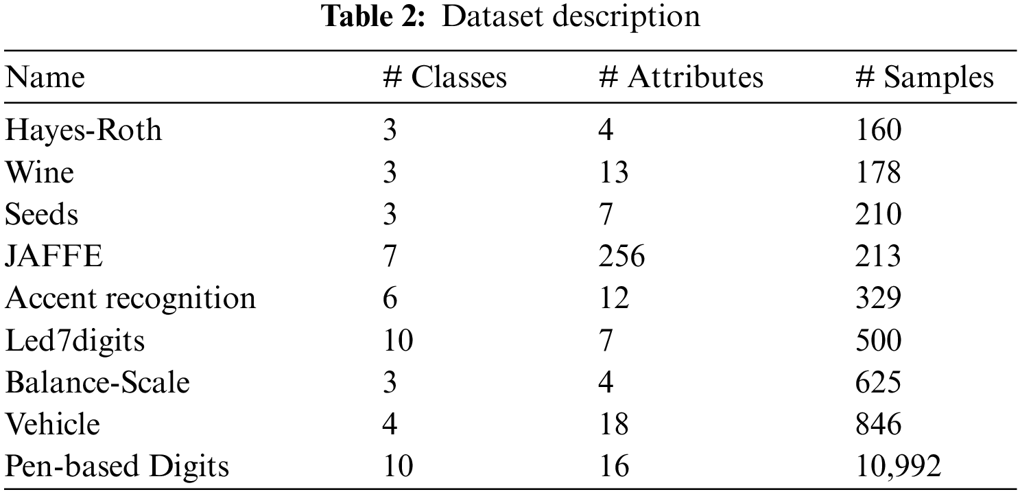
Eight multi-class classification data sets selected from UCI Repository are used in this research. The names of the datasets are as follows: Seeds, Wine, Balance Scale, Hayes Roth, Accent recognition, JAFFE, and Vehicle. Hayes-Roth is the dataset for human subjects’ transfer test. The data has four attributes namely: hobby, age, educational level, and marital status. The class is divided into nominal value between 1 and 3. Wine is the dataset of chemical analysis results of wine grown in Italy derived from three cultivars but have same region. The attributes include 13 constituents quantities found during analysis. Seeds dataset consists of 7 geometric parameters of wheat kernels belonging to 3 different varieties of wheat: Rosa, Kama, and Canadian. JAFFE is the image dataset of 10 Japanese female expressers with 7 posed expressions: happy, sad, fear, angry, disgusting, surprised, and neutral. The dataset consists of 210 images of 256 pixels. Speaker accent recognition is an audio dataset of people accents belonging to 6 countries: Spain, Georgia, France, Italy, United Kingdom, and United States of America. Led7digits is a dataset of LED display with 7 light-emitting diodes hence there are 7 Boolean attributes having 10 concepts ranging between 0 and 9. Balance Scale is the dataset classified according to the balance scale tip which is to the right, left or balanced. Vehicle is the dataset of silhouette of 4 types of vehicles: opel, saab, bus, and van. Different angle of views were taken to classify vehicles according to 18 attributes. Pen-based recognition of handwritten digits is the dataset of 10 digits between 0 and 9 written by 44 writers with 16 attributes having integers ranging between 0 and 100. These data sets are medium-sized ranging from 160 to 10,992 samples. Data sets with diverse characteristics having different numbers of input features, attributes, and classes are selected to analyze the effectiveness of the proposed algorithm with varied constraint conditions. The number of classes and number of attributes of these data sets is in the range of 3–10 and 4 256 respectively. Description of the datasets is given in Tab. 2. Preprocessing of input features is done through normalization to get a symmetric and fast converging cost function. Classification accuracy is used as a metric to evaluate the performance of the E-CGMKL method.

4.2 Competing Algorithms

The proposed scheme is compared with six baseline methods: CGMKL, BPNN, kerNET, SVM (OVO), SVM (OVR), and Random Forest. A brief description of baseline methods is given below:

•   CGMKL: collaborative and geometric multi-kernel learning, the reference method in which multiple RBF kernels are utilized.

•   BPNN: backpropagation neural network with hidden layers, where the final output is extracted from the last layer as in MLP architecture.

•   kerNET: an ensemble algorithm that utilizes EASYMKL for a combination of base kernels then SVM learning is used to train the model.

•   SVM (OVA): support vector machines (one vs. all), it is a classical method that splits the data into multiple binary classification problems and then binary classifiers are trained for each problem to classify multi-class data.

•   SVM (OVO): support vector machines (one vs. one), it is a classical method that splits the multiclass data into binary classification problems for a single class vs. every other class to classify multi-class data.

•   Random Forest: it is the state-of-the-art multi-class classification algorithm involving decision trees. It follows an ensemble learning approach.

4.3 Experimental Setting

In experiments, 5 fold cross-validation is used in which data is divided into 5 folds from which 4 folds are used for training and the remaining 1 fold is used for testing. This process is repeated until each fold is used for testing and then the final result is evaluated by taking the average of test accuracies obtained from each of the five folds. The same partition is used for 5 fold cross-validation for each of the competing algorithms to get unbiased results. To train BPNN the number of hidden layers is set to 2 and the number of neurons per layer is set to 50 and 25 for the first and second layers respectively. ADAM is used as an optimization algorithm and ReLU is used as an activation function. Training of the BPNN is stopped when the loss function converges. For CNN architecture, two convolutional layers are used with 6 and 12 5 × 5 filters respectively. After each convolutional layer, two Max-pool layers are used having a size of 1x1 with a stride of 2. After the Convolutional and Max-pool layers, a dense layer is placed with 128 neurons. Since 2 hidden layers are used, the trained DNN gives 3 base kernels. The proposed algorithm gives the best result using 3 kernels that is why 2 hidden layers are used in DNN. The learning rate of E-CGMKL α is set to 0.01. RMSProp parameters γ,β, and ϵ are set to 0.1, 0.9, and 10−8 respectively. The controlling parameters of regularization terms δ and σ are selected from [0.01,0.1,1,10,100]. The learning of E-CGMKL is stopped when the difference of two consecutive losses is below the threshold value of 10−4. In kerNET, base kernels are combined through the EasyMKL algorithm. EasyMKL has a hyperparameter λ, the value of λ is selected from [0,0.1,0.2,0.5,0.9,1]. For class prediction, kerNET employs SVM (OVO). SVM (OVO) contains the hyperparameter C whose value is selected from [10n,n=−3…3]. The proposed method is also compared with SVM (OVO) and SVM (OVR). These algorithms have hyperparameters C and gamma respectively. The value of C and gamma is selected from {0.01,0.1,1,10,100}. The RBF kernel is used in both SVM (OVO) and SVM (OVR). In the Random forest algorithm, the number of decision trees is set to 100. Parameters of classification algorithms selected for comparison with E-CGMKL are adjusted to get the highest accuracy results. The hyperparameters of all the algorithms are selected using k-fold cross-validation.

5  Results

Tab. 3 presents the testing accuracy of all the classification algorithms used for comparison. As can be seen from Tab. 3, BPNN and Random forest do not show improvement in performance as compared to CGMKL. However, SVM (OVO) and SVM (OVR) lead to significant improvement in average test accuracy compared to CGMKL. E-CGMKL outperforms all the competing algorithms in terms of test accuracy averaged over all datasets. E-CGMKL also achieves higher test accuracy compared to the other methods in 7 out of 9 datasets. Compared to the benchmark CGMKL method, E-CGMKL shows a 1.33% improvement in average test accuracy. This indicates the benefit of constructing multiple kernel spaces from the hidden layers of the trained neural network. As compared to BPNN, E-CGMKL shows an improvement of 2.1% test accuracy. This also indicates the advantage of exploiting intermediate representations of the hidden layers instead of using the output layer for classification results. E-CGMKL also outperforms the KerNET algorithm which demonstrates the crucial role played by the CGMKL algorithm in imposing the consistency constraint across multiple kernel spaces as well as preserving a geometric feature suitable for classification. Compared to Random Forest, E-CGMKL shows an improvement of 6.12% test accuracy. As can be seen from Tab. 3, E-CGMKL gives better test accuracy compared to SVM (OVO), SVM (OVR), and Random Forest in 7 out of 9 data sets. Fig. 4 shows the test accuracies of data sets individually and Fig. 5 shows the average test accuracy results.

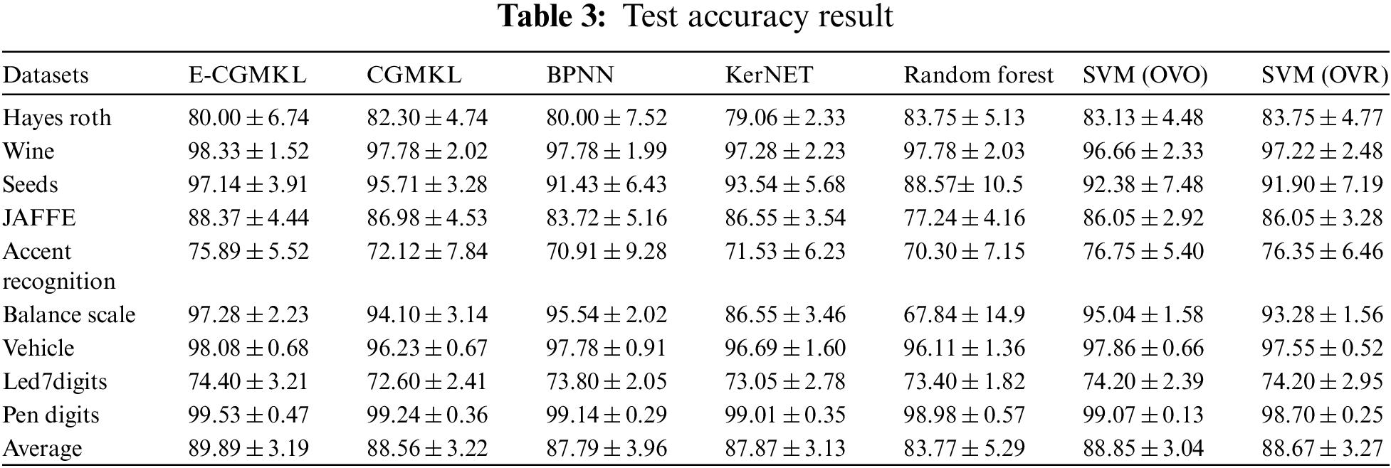
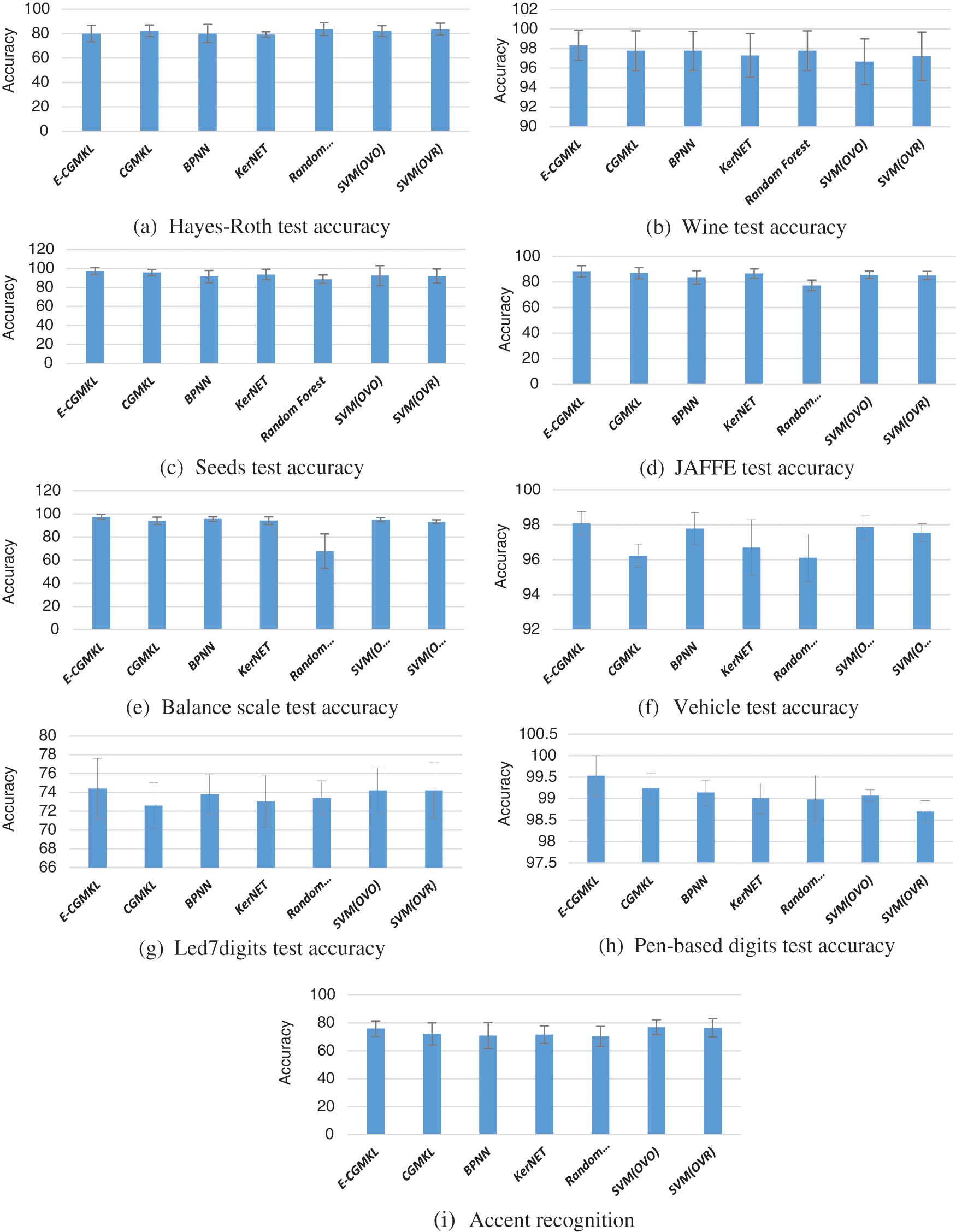
Figure 4: Test score of used data sets on multi-class classification

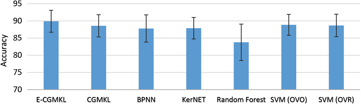
Figure 5: Average test score of comparison algorithms

5.1 Parameter Analysis

As discussed in the methodology section, δ is the parameter that controls the importance of RTSnregularization term in Eq. (2). To exhibit a geometric feature of classification results this term reduces the within-class distance. To illustrate the role of parameter δ the data set having three classes is taken as shown in Fig. 6. The red square, the blue star, and the black triangular represent classes one, two, and three respectively. Fig. 6 shows the change in the distribution of points in kernel space for the three classes as the value of δ increases. The sub-figure (a) demonstrates the original untrained data set. The value of σis fixed to 0.01 and the value of δis varied from 0.01 to 100. The sub-figures from (b) to (f) in Fig. 6 show that by increasing the value of δ the points belonging to the same class form a tight cluster in the high dimensional kernel space. These plots demonstrate the effect of RTSn regularization term on the distribution of class-specific points in the kernel space. Experiments reveal that classification performance with smaller values of δand σis better as compared to larger values.

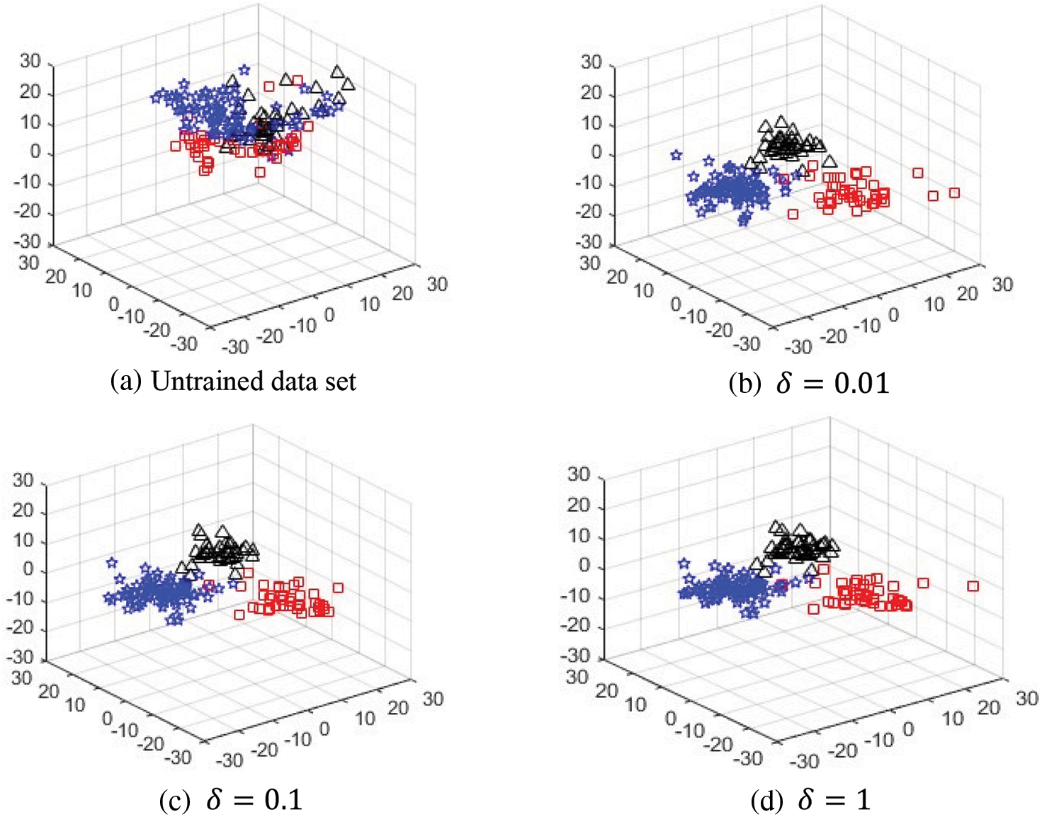
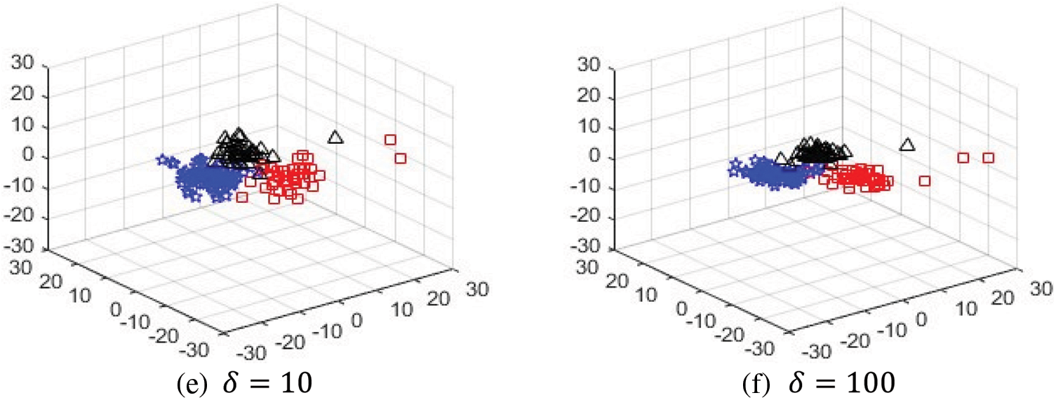
Figure 6: Visualizing the significance of the regularization term δ sub-figure (a) shows the original data set and other sub-figures show how classes with the same colors come closer when the value of δ increases gradually

5.2 Convergence Comparison of E-CGMKL and CGMKL

This section discusses the convergence behavior of E-CGMKL and CGMKL. To accelerate the gradient descent algorithm RMSProp is used in both algorithms. The convergence of both the algorithms on all data sets can be seen in Fig. 7. It is evident from the graphs that convergence of E-CGMKL is faster as compared to the CGMKL algorithm, especially, the convergence rate of E-CGMKL on Hayes Roth, Balance scale, and vehicle datasets is significantly faster than CGMKL.

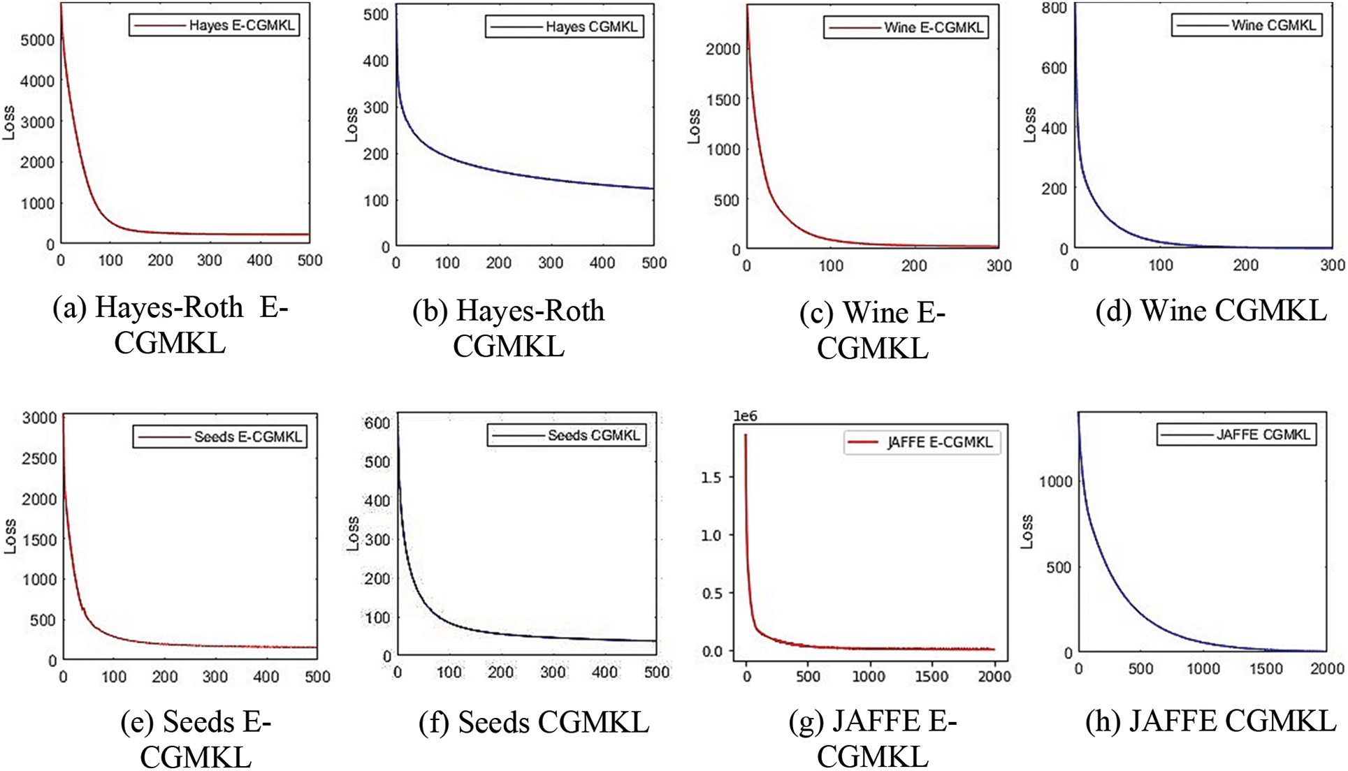
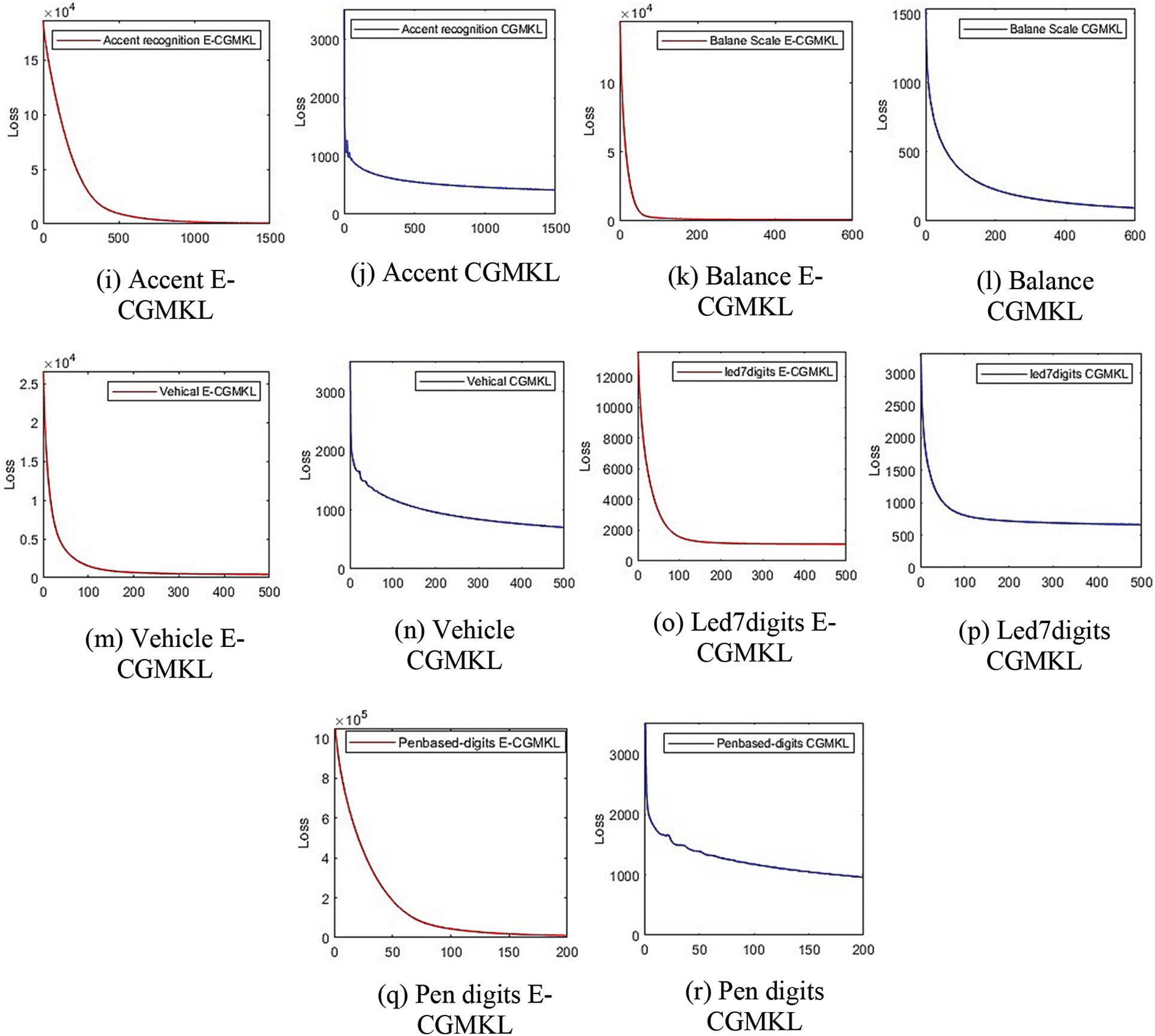
Figure 7: Convergence comparison of E-CGMKL and CGMKL. In the sub-figures of convergence graphs x axis represents the number of iterations and y axis represents the loss after each iteration

6  Conclusion

This paper proposes the E-CGMKL algorithm which enhances the CGMKL algorithm to classify multi-class data with nonlinear data distribution. The softmax function is a good state-of-the-art method to do multi-class classification for linearly distributed data, but when the decision boundary is nonlinear it suffers from performance degradation. Hence, to deal with nonlinear data, CGMKL combines softmax function with multi-kernel learning using the MEKL framework constructed from RBF kernels. In which EKM are feature vectors Φn(x) corresponding to each data sample x. However, kernel spaces constructed in the CGMKL algorithm do not have any explicit relationship as they are constructed by independently setting the width parameter of the RBF kernel to different values. On the other hand, the kernel spaces constructed by the E-CGMKL algorithm inherit the compositional hierarchy of the DNN hidden layers and more effectively capture any complex latent structure in the data set. These hierarchical kernel spaces improve the performance of the CGMKL algorithm significantly on complex datasets such as image data sets. CGMKL ensures consistent outputs of samples across kernel spaces and minimizes the within-class distance to highlight the clustering of different classes. E-CGMKL combines the consistency and cluster preserving aspects of CGMKL with the hierarchical structure of kernel spaces extracted from DNN hidden representations to enhance its predictive performance. The experimental results on various data sets demonstrate the superior performance of the E-CGMKL algorithm compared to other competing methods including the benchmark CGMKL. The performance of E-CGMKL is further enhanced on image classification datasets as these data sets possess complex latent structure which is effectively captured by kernel spaces constructed from CNN. Possible future directions for our work include using parameterized activation functions to construct kernel spaces from DNN and employing transfer learning to efficiently construct kernel spaces for small-sized data sets.

Acknowledgement: I would like to give special thanks to my friend, Mariam Naveed for supporting me in my work.

Funding Statement: The authors received no specific funding for this study.

Conflicts of Interest: The authors declare that they have no conflicts of interest to report regarding the present study.

References

 1.  N. Mehra and S. Gupta, “Survey on multiclass classification methods,” Journal of Computer Science and Information Technologies, vol. 4, pp. 572–576, 2013. [Google Scholar]

 2.  M. Galar, A. Fernández, E. Barrenechea, H. Bustince and F. Herrera, “An overview of ensemble methods for binary classifiers in multi-class problems: Experimental study on one-vs-one and one-vs-all schemes,” Pattern Recognition, vol. 44, pp. 1761–1776, 2011. [Google Scholar]

 3.  B. Krawczyka, M. Galar, M. Wozniak, H. Bustince and F. Herrera, “Dynamic ensemble selection for multi-class classification with one-class classifiers,” Pattern Recognition, vol. 83, pp. 34–51, 2018. [Google Scholar]

 4.  J. A. Saez, M. Galar and B. Krawczyka, “Addressing the overlapping data problem in classification using the one-vs-one decomposition strategy,” IEEE Access, vol. 7, pp. 83396–83411, 2019. [Google Scholar]

 5.  I. Mendialdua, J. M. M. Otzeta, I. R. Rodriguez, T. R. Vazquez and B. Sierra, “Dynamic selection of the best base classifier in one versus one,” Knowledge-Based Systems, vol. 85, pp. 298–306, 2015. [Google Scholar]

 6.  I. Goodfellow, Y. Bengio and A. Courville, Deep Learning, Massachusetts, London, England: MIT Press Cambridge, 2016. [Google Scholar]

 7.  H. Xiong, M. N. S. Swamy and M. O. Ahmad, “Optimizing the kernel in the empirical feature space,” IEEE Transactions on Neural Networks, vol. 16, pp. 460–474, 2005. [Google Scholar]

 8.  Z. Wang, Z. Zhu and D. Li, “Collaborative and geometric multi-kernel learning for multi-class classification,” Pattern Recognition, vol. 99, pp. 107050, 2019. [Google Scholar]

 9.  S. Mahapatra, “Why deep learning over traditional machine learning?” Towards Data Science, 2018. [Google Scholar]

10. I. Lauriola, C. Gallicchio and F. Aiolli, “Enhancing deep neural networks via multiple kernel learning,” Pattern Recognition, vol. 101, pp. 107194, 2020. [Google Scholar]

11. T. Wang, L. Zhang and W. Hu, “Bridging deep and multiple kernel learning: A review,” Information Fusion, vol. 67, pp. 3–13, 2021. [Google Scholar]

12. K. R. Müller, S. Mika, G. Rätsch, K. Tsuda and B. Schölkopf, “An introduction to kernel-based learning algorithms,” IEEE Transactions on Neural Networks, vol. 12, no. 2, pp. 181–201, 2001. [Google Scholar]

13. T. Hofmann, B. Scholkopf and A. J. Smola, “Kernel methods in machine learning,” The Annals of Statistics, vol. 36, pp. 1171–1220, 2008. [Google Scholar]

14. T. Wang, S. Tian, H. Huang and D. Deng, “Learning by local kernel polarization,” Neurocomputing, vol. 72, no. 13–15, pp. 3077–3084, 2009. [Google Scholar]

15. T. Wang, D. Zhao and S. Tian, “An overview of kernel alignment and its applications,” Artificial Intelligence Review, vol. 43, pp. 179–192, 2012. [Google Scholar]

16. J. Li, Y. Liu, H. Lin, Y. Yue and W. Wang, “Efficient kernel selection via spectral analysis,” International Joint Conference on Artificial Intelligence, pp. 2124–2130, 2017. [Google Scholar]

17. T. Wang and W. Li, “Kernel learning and optimization with hilbert–schmidt independence criterion,” Journal of Machine Learning and Cybernetics, vol. 9, pp. 1707–1717, 2017. [Google Scholar]

18. M. Gonen and E. Alpaydın, “Multiple kernel learning algorithms,” Journal of Machine Learning Research, vol. 12, pp. 2211–2268, 2011. [Google Scholar]

19. S. S. Bucak, R. Jin and A. K. Jain, “Multiple kernel learning for visual object recognition: A review,” IEEE Transactions on Pattern Analysis and Machine Intelligence, vol. 36, no. 7, pp. 1354–1369, 2014. [Google Scholar]

20. S. Niazmardi, B. Demir, L. Bruzzone, A. Safari and S. Homayouni, “Multiple kernel learning for remote sensing image classification,” IEEE Transactions on Geoscience and Remote Sensing, vol. 56, no. 3, pp. 1425–1443, 2018. [Google Scholar]

21. A. Rakotomamonjy, F. R. Bach, S. Canu and Y. Grandvalet, “Simplemkl,” Journal of Machine Learning Research, vol. 9, pp. 2491–2521, 2008. [Google Scholar]

22. F. Aiolli and M. Donini, “Easymkl: A scalable multiple kernel learning algorithm,” Neurocomputing, vol. 169, pp. 215–224, 2015. [Google Scholar]

23. M. A. Perez, M. C. Oveneke and H. Sahli, “Svrg-mkl: A fast and scalable multiple kernel learning solution for features combination in multi-class classification problems,” IEEE Transactions on Neural Networks, vol. 31, no. 5, pp. 1710–1723, 2020. [Google Scholar]

24. Y. Han, K. Yang, Y. Ma and G. Liu, “Localized multiple kernel learning via sample-wise alternating optimization,” IEEE Transactions on Cybernetics, vol. 44, no. 1, pp. 137–148, 2014. [Google Scholar]

25. X. Liu, L. Wang, J. Zhang and J. Yin, “Sample-adaptive multiple kernel learning,” IEEE Access, vol. 8, pp. 39428–39438, 2014. [Google Scholar]

26. C. Du, C. Du, G. Long, X. Jin and Y. Li, “Efficient bayesian maximum margin multiple kernel learning,” Machine Learning and Knowledge Discovery in Databases, vol. 3, pp. 165–181, 2016. [Google Scholar]

27. Q. Fan, Z. Wang, H. Zha and D. Gao, “Mreklm: A fast multiple empirical kernel learning machine,” Pattern Recognition, vol. 61, pp. 197–209, 2017. [Google Scholar]

28. L. Breiman, “Random forest,” Machine Learning, vol. 45, pp. 5–32, 2001. [Google Scholar]

29. P. Palimkar, R. N. Shaw and A. Ghosh, “Machine learning technique to prognosis diabetes disease: Random forest classifier approach,” International Conference Advanced Computing and Intelligent Technology, vol. 218, pp. 218–244, 2022. [Google Scholar]

30. G. Liu, L. Tian and W. Zhou, “Multiscale time-frequency method for multiclass motor imagery brain computer interface,” Computer in Biology and Medicines, vol. 143, pp. 105299, 2022. [Google Scholar]

31. H. Nazerian, A. Shirazy, A. Shirazi and A. Hezarkhani, “Design of an artificial neural network (bpnn) to predict the content of silicon oxide (SiO2) based on the values of the rock main oxides: Glass factory feed case study,” International Journal of Science and Engineering Applications, vol. 11, no. 2, pp. 41–44, 2022. [Google Scholar]

32. F. J. Huang and Y. LeCun, “Large-scale learning with SVM and convolutional nets for generic object categorization,” in IEEE Computer Society Conf. on Computer Vision and Patteren Recognition, New York, pp. 284–291, 2006. [Google Scholar]

33. P. Chagas, L. Souza, I. Araujo, N. Aldeman, A. Duarte et al., “Classification of glomerular hypercellularity using convolutional features and support vector machine,” Artificial Intelligence in Medicine, vol. 103, pp. 101808, 2020. [Google Scholar]

34. J. Mairal, P. Koniusz, Z. Harchaoui and C. Schmid, “Convolutional kernel networks,” Advances in Neural Information Processing Systems, vol. 27, pp. 2627–2635, 2014. [Google Scholar]

35. M. Reza, M. Qaraei, R. Monsefi and K. G. Shirazi, “Convolutional kernel networks based on a convex combination of cosine kernels,” Pattern Recognition Letters, vol. 116, pp. 127–134, 2017. [Google Scholar]

36. A. G. Wilson, Z. Hu, R. Salakhutdinov and E. P. Xing, “Deep kernel learning,” Proceedings of Machine Learning Research, vol. 51, pp. 370–378, 2016. [Google Scholar]

37. N. Jean, S. M. Xie and S. Ermon, “Semi-supervised deep kernel learning: Regression with unlabeled data by minimizing predictive variance,” Neural Information Processing Systems, vol. 31, pp. 5327–5338, 2019. [Google Scholar]

38. G. Dai, X. Zhang, X. He and X. Chen, “Tbe-net: A three-branch embedding network with part-aware ability and feature complementary learning for vehicle re-identification,” IEEE Transactions on Intelligent Transportation Systems, vol. 23, pp. 1–13, 2021. [Google Scholar]

39. W. Sun, L. Dai, X. R. Zhang, P. S. Chang and X. Z. He, “Rsod: Real-time small object detection algorithm in UAV-based traffic monitoring,” Applied Intelligence, vol. 51, pp. 1–16, 2021. [Google Scholar]

This work is licensed under a Creative Commons Attribution 4.0 International License, which permits unrestricted use, distribution, and reproduction in any medium, provided the original work is properly cited.