DOI:10.32604/cmc.2022.027947
| Computers, Materials & Continua DOI:10.32604/cmc.2022.027947 | |
| Article |
Online Rail Fastener Detection Based on YOLO Network
1Beijing Key Laboratory of Work Safety Intelligent Monitoring, School of Electronic Engineering, Beijing University of Posts and Telecommunications, Beijing, 100876, China
2Dublin City University, Dublin, 9, Ireland
*Corresponding Author: Yifei Wei. Email: weiyifei@bupt.edu.cn
Received: 29 January 2022; Accepted: 23 March 2022
Abstract: Traveling by high-speed rail and railway transportation have become an important part of people’s life and social production. Track is the basic equipment of railway transportation, and its performance directly affects the service lifetime of railway lines and vehicles. The anomaly detection of rail fasteners is in a priority, while the traditional manual method is extremely inefficient and dangerous to workers. Therefore, this paper introduces efficient computer vision into the railway detection system not only to locate the normal fasteners, but also to recognize the fasteners states. To be more specific, this paper mainly studies the rail fastener detection based on improved You can Only Look Once version 5 (YOLOv5) network, and completes the real-time classification of fastener states. The improved YOLOv5 network proposed contains five sections, which are Input, Backbone, Neck, Head Detector and a read-only Few-shot Example Learning module. The main purpose of this project is to improve the detection precision and shorten the detection time. Ultimately, the rail fastener detection system proposed in this paper is confirmed to be superior to other advanced algorithms. This model achieves on-line fastener detection by completing the “sampling-detection-recognition-warning” cycle of a single sample before the next image is sampled. Specifically, the mean average precision of model reaches 94.6%. And the model proposed reaches the speed of 12 ms per image in the deployment environment of NVIDIA GTX1080Ti GPU.
Keywords: Fastener detection; deep learning; state recognition; real-time classification
The intelligent revolution based on neural network has given new power to many industrial fields, such as automatic control system, intelligent data cache policy for mobile edge networks based on deep Q-learning method [1], heartbeat classification in electronic health using deep learning algorithm [2], cognitive image steganography protocols integrated with machine learning [3], introducing automatic learning algorithms for user scheduling and resource allocation in wireless networks [4]. As an important branch in the field of artificial intelligence, object detection technology has been applied more and more in daily life, such as automatic driving, pedestrian detection, large-scale scene recognition, etc. Therefore, the paper investigates the application of object detection technology in railway safety inspection, and makes the railroad track flaws detection more efficient and ensure the safety of railway transportation. While improving the accuracy of the algorithm, researchers also need to expand the scope of target detection technology and super-resolution image data matching [5]. Track safety has always been a major theme of research all over the world, and the fastener is one of the important parts of the track. The state of fastener determines the rail safety, a missing or incomplete fastener will cause a significant hidden risk to the possessions of owner, and even may appear a major safety accident.
Early detection of rail fastener mainly accomplished by manual inspecting. Workers made inspection tour on a regular time to find out whether there were abnormal phenomena. But there are many drawbacks of artificial detection: (1) Human eye fatigue occurs over a long period of time, so the overall reliability is low. (2) Nowadays the running speed of railway transportation is fast, there is no extra time for manual inspection. (3) The safety of the workers cannot be guaranteed. Apart from the most traditional manual methods, there are some automatic detection methods for fasteners internationally. Automated testing methods mainly include: rail detection based on ultrasonic method [6], fastener detection based on the eddy current testing method [7], fastener detection based on pressure detecting [8], fastener detection based on computer vision [9], etc. The first three methods are based on traditional industrial testing methods, but due to difficulties in physical layer, the detection accuracy and detection speed cannot achieve good results. Furthermore, the implementation cost of pressure detecting and other methods is too high. Therefore, more attention is focused on computer vision technology, and this paper is also based on this direction. Currently, commonly used computer vision detectors are mainly divided into one-stage detectors and two-stage detectors. The two-stage detectors are mainly RCNN (Regions with Convolutional Neural Network features) series, such as FAST-RCNN [10], Faster-RCNN [11] et al. The first step is to generate the suggestion box through object proposal and extract the content in the suggestion box through Backbone. The second step is to use linear classifier such as Supported Vector Machine (SVM). RCNN series have tedious training steps and slow training process. Although they have high detection accuracy, some industry that needs to be lightweight to deployed on mobile terminals and real-time to response issues quickly. As for the one-stage-detection, Single Shot Multi-Box Detector (SSD) [12], which shows a great balance between accuracy and speed, is based on position regression for depth learning image detection. The basic size of the prior box in the SSD network cannot be learned directly, but needs to be set manually. However, the size and shape of the prior box used by each feature layer are exactly different, resulting in the debugging process relying heavily on researchers’ experience. YOLO series [13] have better performance with 24 convolution layers which are responsible for extracting features and 2 fully connected layers. YOLO series as the fastest detection algorithm are often used in various fields. Finally, Non-Maximum Suppression (NMS) [14] is used to solve the problem that there are multiple repeating frames in the same target. In any detector, whether one-stage or two-stage, the most time-consuming step is the feature extraction [15].
The method based on deep learning is gradually applied to automatic detection of rail fasteners. Li [16] proposed an improved SSD fastener positioning algorithm using non-maximum weighted suppression method to replace the original suppression method. After adding residual network to avoid manually adjust the prior box parameters, the improved SSD algorithm reached 90.2% accuracy and speed of 36 FPS. Long [17] used Faster RCNN to build a high-speed rail fastener detection system, but its network structure had a huge amount of computation, resulting in a slow detection speed. The authors in [18] used YOLO network to locate fasteners, but the recognition effect for small targets and the generalization ability were both average. In addition, the detection speed of this paper is only 54 FPS, and the test dataset is too small to prove the true performance of its model.
According to the present research situation, this paper proposes an On-line Fastener Detection method based on computer vision, which mainly uses image processing algorithm to locate and identify fasteners for track images collected from real scenes. Based on YOLO network, the proposed model can effectively detect railway fasteners in different states. This paper adds read-only Few-Shot Example Learning model to the algorithm based on YOLOv5 detection framework. In addition, the details of YOLOv5 network are adjusted to optimize the method for the practical problems in this paper. This method is robust to almost all complex situations faced by high-speed railway system.
In the process of training the object detection model, it is necessary to carefully study the composition of the loss function. In practice, this paper mainly uses two loss calculation methods: Cross Entropy Loss [19] and Focal Loss [20].
Eq. (1) is the calculation method of Cross Entropy function. Cross Entropy Loss is mainly used to judge the loss caused by object classification, and this function will be used to calculate the loss in the classical binary classification problem.
In Eq. (1)
With the above formula, this paper can basically solve the loss caused by classification in some simple scenes. However, in some complex specific scenes, there are some similar samples that are difficult to distinguish. In addition, most of the one-stage detectors enjoy the speed increase brought by the generation of region proposal network, and at the same time, they will also be affected by the decline of receiving accuracy. Therefore, Focal Loss is used as in Eq. (3).
In the above formula, the parameter
After the training dataset enters YOLO network, the output of feature map with fixed structure is generated, including the specific coordinates and size of the predicted bounding box, and the confidence of its classification. The loss is calculated with the output and the manually labeled information, and then the regression optimization of related algorithms is carried out for the overall loss after calculating the loss function. YOLOv5 defines the loss function as Eq. (4) below.
YOLOv5 loss calculation process is mainly divided into two parts, namely regression loss caused by bounding box position (the first item in Eq. (4)) and classification loss. The classification loss is divided into three parts, namely, the loss caused by whether the predicted bounding box contains object (the second and third items in Eq. (4)) and the loss caused by the predicted category probability of objects (the fourth item in Eq. (4)).
The first item is the loss of the predicted bounding box position, which respectively represent the loss caused the differences between the predicted bounding box and the ground truth bounding box.
The latter three items are about the loss caused by classification probability with Binary Cross Entropy Loss.
The last item is the category probability of each bounding box using Binary Cross Entropy.
YOLOv5 draws lessons from the multi-scale feature recognition of SSD and the concept of anchor in two-stage detector, and generates multiple anchors in the same position, so it can generate multiple prediction bounding boxes and improve the recognition ability of small objects. In practical application, the appropriate backbone will be selected as the support according to the needs, so that the detection of the network is faster and more accurate, and at the same time, it can meet the requirements of lightweight.
In this paper, an On-line Railway Fastener Detection system based on improved YOLOv5 is proposed. The data sampling module transmits the acquired depth map to the server through UDP communication in real time. The proposed system performs fastener detecting and state prediction online, and continues to transmit information such as predicted bounding box, confidence level and object category to the total server. The model structure is shown in Fig. 1.

Figure 1: The improved YOLOv5 network of fastener detection
As mentioned above, the data image of the input part of this paper is PNG format with the size of 1280*1000. After image scaling and filling, the data of 640*640*1 is obtained and transmit into the Backbone module in Fig. 1. There is a down-sampling mechanism in Backbone, which makes the three features with specific sizes generated in Head detector, 80*80*27, 40*40*27 and 20*20*27, respectively. 27 stands for (5 + 4)*3, where 5 stands for the five-dimensional information of the length and width, center coordinates and confidence of the output detection boxes, 4 stands for the four fastener categories in this paper, and 3 stands for the number of anchors established in YOLOv5. The model proposed will be briefly described from five parts in Fig. 1.
3.1.1 Improved Mosaic Data Augmentation
The Input structure of YOLOv5 adopts Mosaic data enhancement [21] which refers to Yun et al. [22] algorithm. Different from the commonly used datasets, due to engineering standards, all kinds of fasteners have the same size. Therefore, this model has improved the data augmentation model of YOLOv5 to some extent, and cancelled the scaling feature of Mosaic augmentation with different proportion of each picture. As shown in Fig. 2, CutMix method randomly put the two samples together, while Mosaic data augmentation method can cut out and scale four original images.
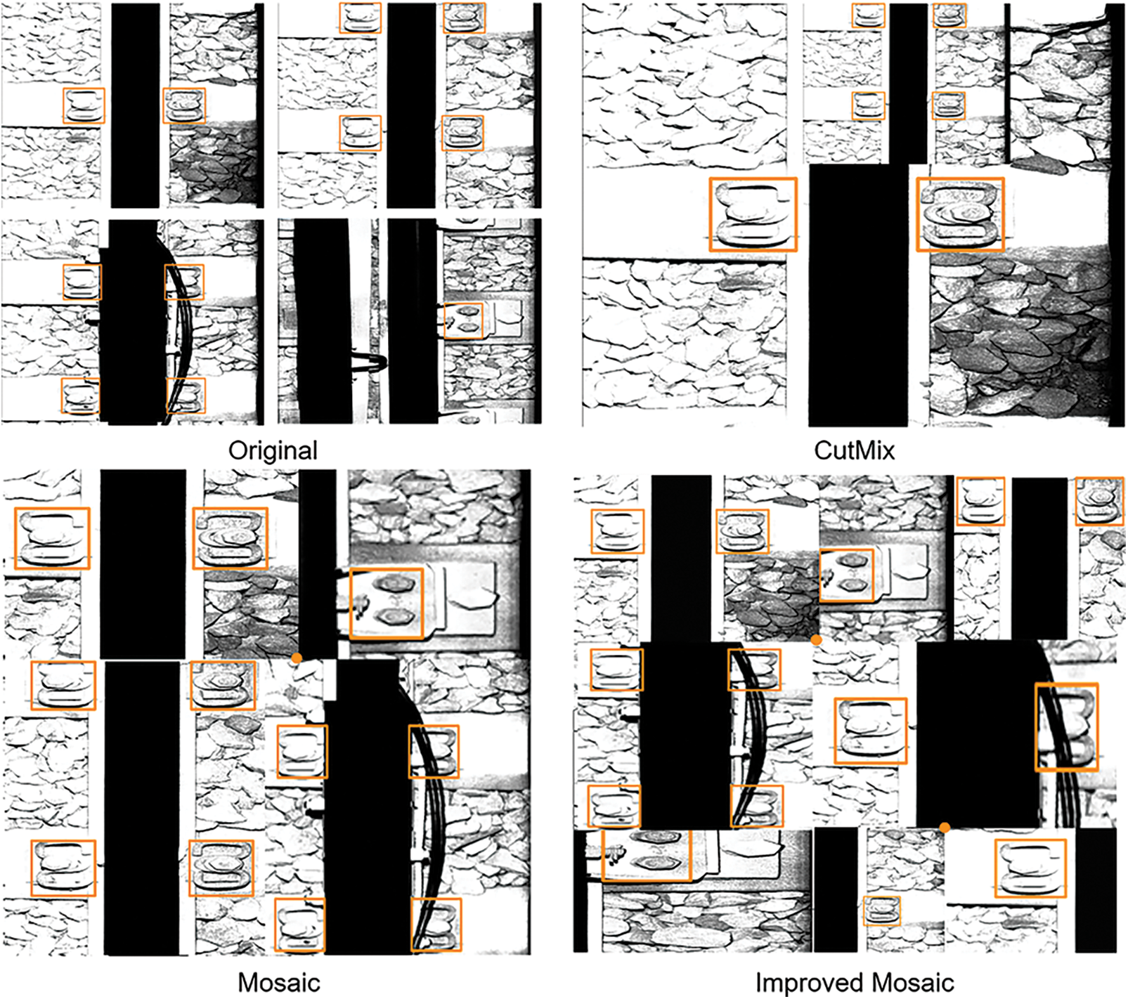
Figure 2: Schematic diagram of three different data augmentation algorithms
The improved Mosaic fixed the ratio of each picture to the new picture after being cut randomly. Considering that the size of the retainer target in this mission is about 250*250, it is about 100*100 in the new image after Mosaic augmentation, which is not a small target. Therefore, based on the improvements mentioned above, this paper tries to combine 9 samples together for Mosaic augmentation, instead of collecting only 4 images. Practically speaking, as shown in Fig. 2, Mosaic augmentation is to randomly select a point near the center of the new image to determine the x and y axes of the matching process of four images. In the improved method mentioned in this paper, the stitching criterion of nine images is to select two points randomly to determine two groups of x and y axes.
Network trained with the improved method converges faster and requires less training time. In this method, the information in the nine pictures will be presented in one picture and fed into the network as a training image. This method makes the network structure lighter and the Input part runs faster. While the detection results are not much different from Mosaic data augmentation, and the robustness of the model is better.
According to different application fields, there are a variety of image sizes. The commonly used method of computer vision is to scale the original image according to the standard size and then send image after processing to the detection network. In this paper, the images of railway track fastener with the size of 1280*1000 are scaled and filled into 640*640*1.
In this paper, the Backbone part of the model mainly uses Focus, CSPDarknet and SPP structures. Fig. 3 shows the simplified Backbone structure, and its core content will be briefly described below.

Figure 3: Simplified structure of YOLOv5 network backbone
The first innovative structure of Backbone is Focus structure, which is mainly used to slice images. In this paper, the original picture of 640*640*1 can be input into a feature map of 320*320*4 after slicing by using YOLOv5s structure. Then, a convolution operation with 32 convolution kernels is performed again, and a feature map of 320*320*4 is obtained. The YOLOv5s model this paper used has Focus structure with size of 3*3 convolution kernel and its output channel is 32. The purpose of Focus module is to reduce the params and FLOPs, so as to achieve the effect of speed.
The system adopted in this paper follows the Backbone module of YOLOv5 model and uses CSPDarknet as the Backbone to extract abundant information features from the input images. Its core contents are DarknetConv2D, Batch Normalization and Leaky ReLU. CSPNet focuses on solving the problem of repeated gradient information of network optimization existed in other large-scale CNN framework Backbone, and integrates the gradient changes into the feature graph from beginning to end, thus reducing the model parameters and FLOPS values, ensuring the reasoning speed and accuracy, and reducing the model size.
Unlike R-CNN, Spatial Pyramid Pooling (SPP) Network first convolves the whole picture and then gets a feature map. Then, each candidate region is mapped with feature map to get the feature vector of each candidate region. Because these size difference of feature vectors, an SSP layer is added. As shown in Fig. 4, the specific application of SPP network in YOLO is to concat the feature maps through the MaxPooling layer of convolution kernel 5, 9 and 13 respectively. The SSP layer can receive feature map input of random size, and output feature vectors of fixed size, then pass them to the full connection layer. By using SPP module, Backbone is more effective to increase the receiving range of trunk features. More importantly, SPP module helps Backbone separate the contextual features.

Figure 4: Spatial Pyramid Pooling network architecture in YOLO network
Inspired by Feature Pyramid Network (FPN) [23], the Neck continues the structure of the originalYOLOV5 using Path Aggregation Network (PAN) [24]. FPN mainly solves the multi-scale problem in object detection. ResNet greatly improves the performance of small object detection after adopting the simple network connection as FPN. As shown in Fig. 5, FPN is roughly divided into three parts, namely, bottom-up sampling and top-down up-sampling and lateral connection. Each layer of the network through these three structures will have strong semantic information, and can well meet the requirements of speed and memory.

Figure 5: The concrete structure of Neck module in YOLOv5 network
PAN accesses behind FPN network in a bottom-up manner as the bottom-up path augmentation in Fig. 5, and transmits the strong positioning features of the lower layer. The FPN layer conveys strong semantic features from top to bottom, while the PAN layer conveys strong positioning features from bottom to top. Specifically, as in FPN backbone, when down-sampling is carried out, new feature map is the element-wise addition result of feature down-sampling and the upper layer’s feature map of new size. The smallest feature map is directly copied from the 20*20 size feature map of the upper layer. The bottom-up path is the same as FPN backbone with up-sampling operation. Consequently, Neck structure aggregates parameters of different detection layers from different trunk layers.
In this paper, YOLOv3 head is used in the same model as YOLOv5, and the improved YOLOv5 model uses Distance-IoU loss function to replace the original IoU loss as in the first item in Eq. (4) mentioned before.
Distance-IoU is a generalized IoU algorithm, and the expression of DIoU is shown in Eq. (5), in which the latter term is a penalty term. As in Eq. (5),

Figure 6: DIoU loss for bounding box regression
The penalty term is used to minimize the distance between the center points of two bounding boxes. Experiments show that D-IoU has good convergence speed and effect, and it also can be used in NMS calculation, considering not only the overlapping area but also the distance between the center points. When the target frame wraps the prediction frame, the distance between the two frames is directly measured, so DIoU_Loss converges faster. Accordingly, the on-line rail fastener positioning system in this paper defines the non -maximum suppression of the prediction box as DIoU_NMS.
As the dataset in this paper is an imbalanced long-tailed dataset, this paper introduces a read-only Few-shot Example Learning (FEL) module as in Fig. 1. Structurally, FEL model is as same as YOLOv5’s original network. The difference between FEL model and original YOLOv5 network is about the input data. As for the rail fasteners in Fig. 7, these types of fasteners cannot be detected easily due to the small number of samples during training. Therefore, the improved YOLOv5 model inputs these few-shot data into the FEL module.

Figure 7: Few-shot examples in rail fastener dataset
The conventional YOLOv5 network carries out forward propagation, which propagates forward and backward propagations in FEL module with few shot samples as input. FEL module synchronizes the residuals learned from few shot samples to the regular YOLOv5 network for weight update. In the testing and detecting stages, only the conventional modules run, which does not affect the testing speed of the improved network.
In this paper, the threshold of IoU is chosen as 0.8, and the experiment is running on two NVIDIA GTX1080Ti GPUs. In this paper, inference time and mean Average Precision (mAP) are used to measure network performance.
One conventional rail data after brightness adjustment is shown in Fig. 8. It is clearly that the rail edge of most data is in the middle of the picture, and the fasteners are symmetrically distributed beside the rail edge. It can be seen from Fig. 9a that the normalized coordinates of the center of the detection bounding boxes predicted by the model are distributed on both sides of the central track as mentioned above, while the size information of the detection bounding box (normalized length and width) is shown in Fig. 9b, showing a large-scale centralized and sporadic abnormal size distribution.
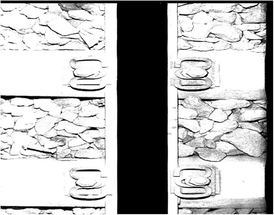
Figure 8: A railway data image in JPG format after brightness adjustment

Figure 9: The distribution of predicted detection boxes in the dataset images
In this paper, four different advanced algorithms are selected for comparison, which are Histogram of Oriented Gradient (HOG) +SVM, Faster R-CNN, MobileNet-SSD, MobileDets and original YOLOv5. To break through the speed bottleneck of region proposal, Faster R-CNN directly uses CNN to generate region proposal by introducing RPN, and shares the convolution layer with CNN in the second stage. HOG is a kind of edge feature, which makes use of the orientation and intensity information of the edge, and is then widely used in visual target detection such as vehicle detection and license plate detection. The combination of HOG and SVM classifier is a common method for locating and detecting rail fasteners in China. The core of SSD method is to use a small convolution filter to predict the category scores and position offsets of a set of default bounding boxes fixed on the feature map. MobileDets [25] is a lightweight object detection algorithm that can be deployed on mobile devices, its most prominent advantage is that it reduced FLOPs and Params to a new level.
When the model proposed in this paper is applied to compare with baseline in the rail fastener dataset, as shown in Tab. 1, the model proposed is superior in two different verification criteria with higher discrimination precision and shorter sample recognition time. In addition to the model proposed in this paper, the original YOLOv5 has obvious advantages in the inference time, while Faster R-CNN confirms its detection accuracy as a two-stage detector with the second highest mAP. MobileDets, known for its lightness, is indeed superior to improved YOLOv5 network proposed in inference time, but its mAP is slightly inferior to the model in this paper.
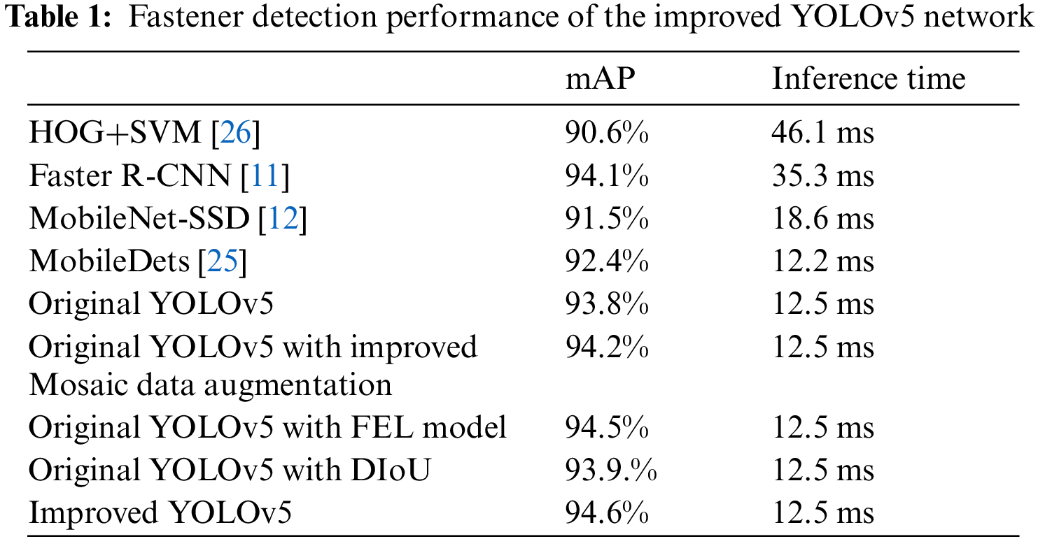
In order to clarify the influence of improvements proposed in this paper, there are several ablation experiments results. As shown in Tab. 1, the three improvements proposed in this paper can improve the mAP of the model in rail Fastener data set to a certain extent. As shown in Tab. 1, the most significant method to promote mAP is the FEL Model proposed in this paper, which has made great progress (0.7%) by increasing the network’s attention to the few-shot examples. DIoU can achieve better detection accuracy (0.1%) in fastener detection than GIoU. Improved Mosaic data augmentation is also helpful to mAP improvement, but its main purpose is to accelerate the convergence speed of the network in training, which will be verified in future work. This paper improves the structure of YOLOv5 to adapt to the rail fastener dataset, and then receives the best performance than other advanced algorithms in the same period.
In this paper, a rail fastener detection system based on improved YOLOv5 is proposed. The FEL model is introduced into YOLOv5 network structure, which enhances the detecting ability of the network for the few-shot samples. Compared with other similar algorithms, the Input and Head modules are improved on the basis of YOLOv5, and better results are obtained. For the specific application scenario [27], the model in this paper gives the whole rail anomaly detection system more relaxed judgment time. This model makes the “sampling-detection-recognition-warning” cycle of a single picture complete before the next picture is collected. The sampling time of a single picture in this paper is about 53 ms, and the shorter detection time means the establishment of a more mature so-called real-time rail fastener anomaly detection system.
Funding Statement: This work was supported by the National Natural Science Foundation of China (61871046, SM, http://www.nsfc.gov.cn/).
Conflicts of Interest: The authors declare that they have no conflicts of interest to report regarding the present study.
1. S. Sun, J. Zhou, J. Wen, Y. Wei and X. Wang, “A DQN-based cache strategy for mobile edge networks,” Computers Materials & Continua, vol. 71, no. 2, pp. 3277–3291, 2022. [Google Scholar]
2. L. Sun, Y. L. Wang, Z. G. Qu and N. N. Xiong, “BeatClass: A sustainable ECG classification system in IoT-based eHealth,” IEEE Internet of Things Journal, vol. 9, pp. 1, 2021. [Google Scholar]
3. Z. G. Qu, H. R. Sun and M. Zheng, “An efficient quantum image steganography protocol based on improved EMD algorithm,” Quantum Information Processing, vol. 20, no. 53, pp. 1–29, 2021. [Google Scholar]
4. Y. Wei, F. R. Yu, M. Song and Z. Han, “User scheduling and resource allocation in HetNets with hybrid energy supply: An actor-critic reinforcement learning approach,” IEEE Transactions on Wireless communications, vol. 17, no. 1, pp. 680–692, 2018. [Google Scholar]
5. L. Xiangchun, C. Zhan, S. Wei, L. Fenglei and Y. Yanxing, “Data matching of solar images super-resolution based on deep learning,” Computers Materials & Continua, vol. 68, no. 3, pp. 4017–4029, 2021. [Google Scholar]
6. R. S. Edwards, S. Dixon and X. Jian, “Characterisation of defects in the railhead using ultrasonic surface waves,” Nondestructive Testing & Evaluation International, vol. 39, no. 6, pp. 475–486, 2006. [Google Scholar]
7. H. M. Thomas, T. Heckel and G. Hanspach, “Advantage of a combined ultrasonic and eddy current examination for railway inspection trains,” OR Insight, vol. 49, no. 6, pp. 341–344, 2007. [Google Scholar]
8. J. J. Zhao, X. B. Zhao, X. H. Li, B. Zhang, B. Wang et al., “Fasteners state detection system based on wireless data transfer module,” Applied Mechanics & Materials, vol. 513, no. 1, pp. 3924–3927, 2014. [Google Scholar]
9. H. Feng, Z. Jiang, F. Xie, P. Yang, J. Shi et al., “Automatic fastener classification and defect detection in vision-based railway inspection systems,” IEEE Transactions on Instrumentation and Measurement, vol. 64, no. 4, pp. 877–888, 2014. [Google Scholar]
10. Y. Chen, W. Li, C. Sakaridis, D. Dai and L. Van, “Domain adaptive faster r-cnn for object detection in the wild,” in Proc. CVPR, Salt Lake City, UT, USA, pp. 3339–3348, 2018. [Google Scholar]
11. S. Ren, K. He, R. Girshick and J. Sun, “Faster R-CNN: Towards real-time object detection with region proposal networks,” IEEE Transactions On Pattern Analysis And Machine Intelligence, vol. 39, no. 6, pp. 1137–1149, 2020. [Google Scholar]
12. D. Biswas, H. Su, C. Wang, A. Stevanovi and W. Wang, “An automatic traffic density estimation using Single Shot Detection (SSD) and MobileNet-SSD,” Physics and Chemistry of the Earth, vol. 110, no. 1, pp. 176–184, 2019. [Google Scholar]
13. W. Sun, G. Z. Dai, X. R. Zhang, X. Z. He and X. Chen, “TBE-Net: A three-branch embedding network with part-aware ability and feature complementary learning for vehicle re-identification,” IEEE Transactions on Intelligent Transportation Systems, vol. 23, pp. 1–13, 2021. [Google Scholar]
14. S. Liu, D. Huang and Y. Wang, “Adaptive NMS: Refining pedestrian detection in a crowd,” in Proc. CVPR, Long Beach, CA, USA, pp. 6459–6468, 2019. [Google Scholar]
15. K. Duan, S. Bai, L. Xie, H. Qi and Q. Huang, “CenterNet: keypoint triplets for object detection,” in Proc. ICCV, Seoul, Korea, pp. 6568–6577, 2019. [Google Scholar]
16. Z. Li, Research on high speed rail fastener detection algorithm based on deep learning, M.S. dissertation, Southwest Jiaotong University, China, 2020. [Google Scholar]
17. Y. Long, Study on detection system of rail fastener based on deep learning, M.S. dissertation, Beijing Jiaotong University, China, 2018. [Google Scholar]
18. W. B. Zhang, S. B. Zheng, P. C. Li and X. Guo, “Positioning algorithm of track images based on YOLO deep convolution network,” Railway Standard Design, vol. 64, no. 9, pp. 22–27, 2020. [Google Scholar]
19. Y. Ho and S. Wookey, “The real-world-weight cross-entropy loss function: modeling the costs of mislabeling,” IEEE Access, vol. 8, pp. 4806–4813, 2019. [Google Scholar]
20. K. Doi and A. Iwasaki, “The effect of focal loss in semantic segmentation of high resolution aerial image,” in Proc. IGARSS, Valencia, Spain, pp. 6919–6922, 2018. [Google Scholar]
21. H. Lv, H. Zhang, C. Zhao, C. Liu, F. Qi et al., “An improved SURF in image Mosaic based on deep learning,” in Proc. ICIVC, Xiamen, China, pp. 223–226, 2019. [Google Scholar]
22. S. Yun, D. Han, S. Chun, S. J. Oh, Y. Yoo et al., “CutMix: Regularization strategy to train strong classifiers with localizable features,” in Proc. ICCV, Seoul, Korea (Southpp. 6022–6031, 2019. [Google Scholar]
23. T. Lin, P. Dollár, R. Girshick, K. He, B. Hariharan et al., “Feature pyramid networks for object detection,” in Proc. CVPR, Honolulu, HI, USA, pp. 936–944, 2017. [Google Scholar]
24. S. Liu, L. Qi, H. Qin, J. Shi and J. Jia, “Path aggregation network for instance segmentation,” in Proc. CVPR, Salt Lake City, UT, USA, pp. 8759–8768, 2018. [Google Scholar]
25. Y. Xiong, H. Liu, S. Gupta, B. Akin, G. Bender et al., “Mobiledets: Searching for object detection architectures for mobile accelerators,” in Proc. CVPR, Nashville, TN, USA, pp. 3825–3834, 2021. [Google Scholar]
26. G. Dai, Research on application of image recognition technology in anomaly detection of rail fasteners, M.S. dissertation, Harbin Engineering University, China, 2018. [Google Scholar]
27. W. Sun, L. Dai, X. R. Zhang, P. S. Chang and X. Z. He, “RSOD: Real-time Small object detection algorithm in UAV-based traffic monitoring,” Applied Intelligence, vol. 92, no. 6, pp. 1–16, 2021. [Google Scholar]
 | This work is licensed under a Creative Commons Attribution 4.0 International License, which permits unrestricted use, distribution, and reproduction in any medium, provided the original work is properly cited. |