Computers, Materials & Continua DOI:10.32604/cmc.2022.028154
Article

Iterative Semi-Supervised Learning Using Softmax Probability

Heewon Chung and Jinseok Lee*

Department of Biomedical Engineering, College of Electronics and Information, Kyung Hee University, Yongin-si, Gyeonggi-do, 17104, Korea
*Corresponding Author: Jinseok Lee. Email: gonasago@khu.ac.kr
Received: 03 February 2022; Accepted: 10 March 2022

Abstract: For the classification problem in practice, one of the challenging issues is to obtain enough labeled data for training. Moreover, even if such labeled data has been sufficiently accumulated, most datasets often exhibit long-tailed distribution with heavy class imbalance, which results in a biased model towards a majority class. To alleviate such class imbalance, semi-supervised learning methods using additional unlabeled data have been considered. However, as a matter of course, the accuracy is much lower than that from supervised learning. In this study, under the assumption that additional unlabeled data is available, we propose the iterative semi-supervised learning algorithms, which iteratively correct the labeling of the extra unlabeled data based on softmax probabilities. The results show that the proposed algorithms provide the accuracy as high as that from the supervised learning. To validate the proposed algorithms, we tested on the two scenarios: with the balanced unlabeled dataset and with the imbalanced unlabeled dataset. Under both scenarios, our proposed semi-supervised learning algorithms provided higher accuracy than previous state-of-the-arts. Code is available at https://github.com/HeewonChung92/iterative-semi-learning.

Keywords: Semi-supervised learning; class imbalance; iterative learning; unlabeled data

1  Introduction

Image classification is a problem to categorize images into one of the multiple classes. It has been considered one of the most important tasks since it is the basis for other computer vision tasks such as image detection, localization and segmentation [1–6]. Since AlexNet [7] was introduced, deep neural networks (DNNs) have evolved remarkably via VGG-16 [8], GoogLeNet [9], ResNet [10], Inception-V3 [11], especially to solve the image classification tasks. DNNs have been widely used for a variety of tasks and set the new state-of-the-art, sometimes even surpassing human performance on image classification tasks.

However, when dealing with the classification problem in practice, we face many practical issues, and one of the most challenging issues is acquiring enough labeled data for training. The acquisition of the labeled data often requires a lot of time while also requiring professional and delicate works. A recent study reported that physicians spent an average of 16 minutes and 14 seconds per encounter using electronic health record (EHRs), with chart review (33%), documentation (24%), and ordering (17%) functions accounting for most of the time [12]. The manual labeling of medical images also requires intensive labor [13,14]. In addition, even if the labeled data is acquired enough, there is another challenging issue referred to as imbalanced dataset. For instance, for the classification of a specific disease data, there is much more information about the data from healthy subjects than those from patients.

To resolve these issues, semi-supervised learning methods using additional unlabeled data have been being considered a lot. Semi-supervised learning is a machine learning approach that combines a small amount of labeled data with a large amount of unlabeled data during training [15–17]. In this study, we propose a novel semi-supervised learning algorithms providing the performance at the level of supervised learning by focusing on automatically and accurately labeling additional unlabeled data. More specifically, to accurately label the unlabeled data, we use a softmax probability as a confidence index and decide whether to assign a pseudo-label to the unlabeled data. The data with labels are used continuously for training. Finally, the process is repeated until the pseudo-labels are assigned to all unlabeled data with high confidence. Our proposed approach is innovative because it effectively and accurately labels the unlabeled data using a simple mathematical function of softmax. For classification problems, softmax is essential part of a model, usually used in the last output layer. Thus, we expect to be able to effectively label the unlabeled data without additional computational complexity.

This paper is organized as follows. Section 2 lists some related works. Section 3 provides a specific motivation of dealing with unlabeled data. In Section 4, we introduce our proposed iterative semi-supervised learning using softmax probabilities. In Section 5, the performance of our algorithm is verified by comparative experiments. The conclusion and future work are described in Section 6.

2  Related Works

The difficulty of acquiring labeled data and the imbalanced data issue have been investigated by many research groups [18–21]. One of the popular approach to handle the imbalanced data issue is with data-level techniques including over-sampling and under-sampling [22–24]. The under-sampling is a technique to balance an imbalanced dataset by keeping all of the data in the minority group and decreasing the size of the majority group. This technique is mainly used when the amount of data belonging to minority and majority groups is large. The over-sampling is a technique to balance an imbalanced dataset by increasing the size of the minority group. This technique is mainly to duplicate minority data by randomly selecting the data from the minority group. A more advanced technique is the synthetic minority oversampling technique (SMOTE), which generates a new data point by selecting a point on a line connecting a randomly chosen minority class sample and one of its k nearest neighbors [25]. Let us denote the synthetic data point by xnew, which can be expressed as

xnew=x+λ⋅(x−xnear),(1)

where x is a random data belonging to a minority group, xnear is one of the k nearest neighbors of x. The parameter λ is independent and identically distributed number uniformly distributed on [0,1]. This SMOTE has the advantage that of being able to increase the size of the minority group without duplicating the data. Similar to SMOTE, adaptive synthetic sampling (ADASYN) technique generates a new data point based on the k nearest neighbors [26]. It generates more data that are harder to learn compared to the data that are easier to learn by considering the data distribution. Thus, it can adaptively shift the decision boundary to focus on the hard-to-learn data. Since the data-level techniques from over-sampling approach balance out the number of each group of data, the trained models have worked well in a variety of applications. However, such over-sampling techniques are available when the data is represented as a vector.

Another approach to handle the imbalanced data issue is with algorithmic methods. In the algorithmic approach, the learning process is adjusted in a way that emphasizes the importance of the minority group data. Most commonly, the cost or loss function is modified to weigh more towards the minority group data or to weigh less towards the majority group data [18,27,28]. Such a sample weighting in loss function is to weigh the loss computed for different samples differently based on whether they belong to the majority or the minority group. For the weight factors, inverse of number of samples or inverse of square root of the number of samples can be considered. Recently, Cui et al. [29] introduced the effective number of samples Enc, which can be defined as

Enc=1−βnc1−β,(2)

where nc is the number of samples in class c and β is a hyperparameter on [0,1]. By using the effective number of samples, the weight factor 1/Enc weigh the loss from the data according to the majority or the minority group. This algorithm approach also worked well in a variety of applications. Nevertheless, the imbalanced dataset issue is not completely solved. The fundamental solution is to increase the number of data with diversity by acquiring more new data.

As we mentioned above, the most challenging part of acquiring data is labeling new data. It not only takes a lot of time, but also requires professional and delicate works. Recently, Yang et al. [30] demonstrated that pseudo-label on extra unlabeled data can improve the classification performance, especially with the imbalanced dataset. The method is based on the fact that the unlabeled data is relatively easy to obtain while the labeled one is difficult to obtain. Based on the trained model with original data, extra unlabeled data was subsequently labeled. Accordingly, it was shown that the trained model with additional unlabeled data provided better performance. However, the pseudo-labels also can be biased towards a majority of data. Thus, the improvement from usage of the extra unlabeled data is limited. In our work, we focus on how to more correctly label the unlabeled data, which eventually provides better performance.

3  Preliminaries and Motivation

Given a simple binary classification from the data PXY with a mixture of two Gaussians, consider that each class data has the label Y:+1or−1. Also, consider the data distribution of X|Y is N(μ1,σ2) when Y=+1. Similarly, when Y=−1, the data distribution of X|Y is N(μ2,σ2), where μ1>μ2. Given one sample x, if x>μ1+μ22, then x can be classified into +1; otherwise −1. Accordingly, the classifier can be expressed as f(x)=sign(x−μ1+μ22), where the term μ1+μ22 needs to be learned based on the data set X and the corresponding label set Y.

However, given imbalanced training data, the term μ1+μ22 in the trained classifier will be shifted to the mean value of a minority class. If a majority of data has the label Y=+1, then the classifier can be derived as f(x)=sign(x+α−μ1+μ22), where α>0. Fig. 1a illustrates an example of a biased classifier, which focuses mainly on improving the classification performance of a majority class. Such a class imbalance issue can be resolved by balancing data class via data sampling approach such as over-sampling or under-sampling as shown in Fig. 1b: in this example, the predicted decision boundary is closer to the actual boundary after using under-or over-sampling method. Similarly, sampling weighting methods also change the predicted decision boundary to the actual boundary.

Fig. 1c illustrates another example of a biased classifier, which focuses on improving the performance of a majority class. However, in this example, the number of data from a minority class is too small to generalize the data corresponding to the minority class. Since the data from the minority class does not generalize to the actual distribution, any sampling approach cannot improve the performance as shown in Fig. 1d: in this example, the predicted decision boundary is almost unchanged even after using under-or over-sampling method. Similarly, sampling weighting methods also have little effect on the predicted decision boundary.

To alleviate the class imbalance issue, Yang et al. [30] recently demonstrated that pseudo-label on extra unlabeled data can improve the classification performance, especially with the imbalanced dataset, theoretically and empirically. More specifically, a base classifier fB was first trained based on the original imbalanced training data. Subsequently, extra unlabeled data was labeled using fB. At last, by re-training fB with the additional pseudo-label data, the classifier was shown to be improved. However, the pseudo-labels also can be biased towards a majority of data, which results in the incorrect labeling, especially for a minority of data. Thus, the improvement from usage of the extra unlabeled data is limited. In this study, we present the algorithms that can improve the labeling accuracy, which eventually improves the overall classification performance.

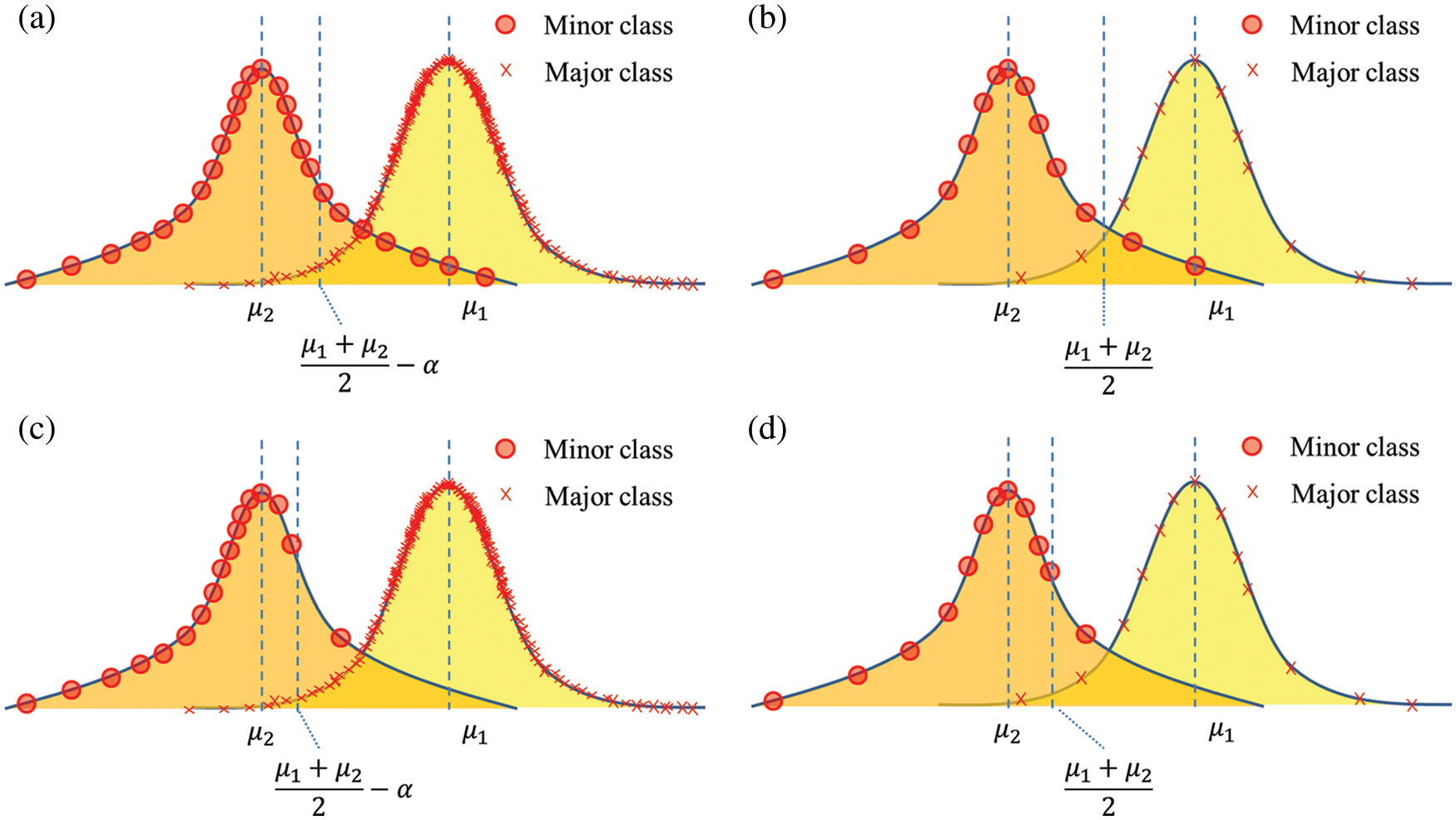
Figure 1: Examples of a biased classifier and the effects of data-level techniques; (a) an example of a biased classifier, (b) the effect of under-or over-sampling method (the predicted decision boundary closer to the actual boundary), (c) another example of a biased classifier, (d) the effect of under-or over-sampling method (little effect on the predicted decision boundary)

4  Iterative Semi-Supervised Learning Using Softmax Probability

4.1 Algorithm Description

In this study, we propose the semi-supervised learning algorithms, which iteratively corrects the labeling of the extra unlabeled data. Algorithm 1 presents the pseudo-code of our proposed algorithm named iterative semi-supervised learning based on softmax probability (ISSL-SP). Let denote the original labeled data and the extra unlabeled data by Dataori and Dataun, respectively. Regarding the instance perspectives, let denote the ith extra unlabeled data and the corresponding label by Datauni and Labeluni, respectively. Let also denote the ith original labeled data and the corresponding label by Dataorii and Labelorii, respectively. Before applying the algorithm ISSL-SP, we first train a base classifier fB using the original training data Dataori. In the first stage, we consider the softmax probabilities corresponding to each class for Datauni, where i=1,2,…n(Datauni) for the number of unlabeled data. For each of Datauni, if the maximum value of the softmax probabilities is equal or greater than 0.99, we assigned the corresponding the class to Labeluni. Here, the optimized threshold value of 0.99 was found throughout this study, and the trade-off between accuracy metrics and the threshold value is described in Results. On the other hand, if the maximum value of the softmax probabilities is less than 0.99, we assign the label Labeluni as undefined. Every iteration, we update fB using all available data for training: fB to fnew. Finally, we arrange the data with labels assigned as undefined, and repeat the entire process until all the data is labeled in a specific class. In this way, ISSL-SP improves the overall classification performance by assigning the labels only with high softmax probability.

4.2 Algorithm Insight

Based on Datauni with Labeluni from fB, let denote the data corresponding to Labeluni=+1 by Datauni+. Similarly, let denote the data corresponding to Labeluni=−1 by Datauni−. As we mentioned above, our aim is to learn μ1+μ22. Here, with Datauni+ and Datauni−, the estimator can be constructed by

θ=12(∑i=1n+Datauni+n++∑i=1n−Datauni−n−),(3)

where n+ and n− are the numbers of the Datauni+ and Datauni−, respectively. Given the distribution of Datauni+N(μ1,σ2), and that of Datauni−N(μ2,σ2), the estimator can be expressed by

θ∼12(∑i=1n+N(μ1,σ2)n++∑i=1n−N(μ1,σ2)n−)(4)

The term σ2(1n++1n−) decreases as n+ and n− increase. Based on the assumption that the unlabeled data is correctly labelled, the estimation accuracy can increase as the number of unlabeled data increases. However, the base classifier fB based pseudo-labels can be biased towards a majority of data. Thus, we need to select only the pseudo-label data with high confidence and to train the model together with Dataori. Then, the base classifier fB can be updated to the model providing higher accuracy, which labels the remained unlabeled data. By repeating the process over and over, the accuracy of the classifier model gradually improves.

4.3 A variant of ISSL-SP

ISSL-SP algorithm can be extended in a variety of forms. Algorithm 2 presents the pseudo-code named ISSL-SP with re-labeling all the initial unlabeled data (ISSL-SPR). As a variant of ISSL-SP, ISSL-SPR is the same as ISSL-SP, except that all of the unlabeled data is labeled again every iteration: the line 18 in ISSL-SP (Algorithm 1) is missing. Since the updated classifier fnew is trained with ever increasing data, it can provide better performance as the process is repeated; and thus, it may be necessary for the initial unlabeled data Dataun to be labeled over and over again. To sum up, ISSL-SP labels only the data assigned by undefined while ISSL-SPR labels all initial unlabeled data over again.

5  Dataset and Experiment Setup

5.1 Dataset

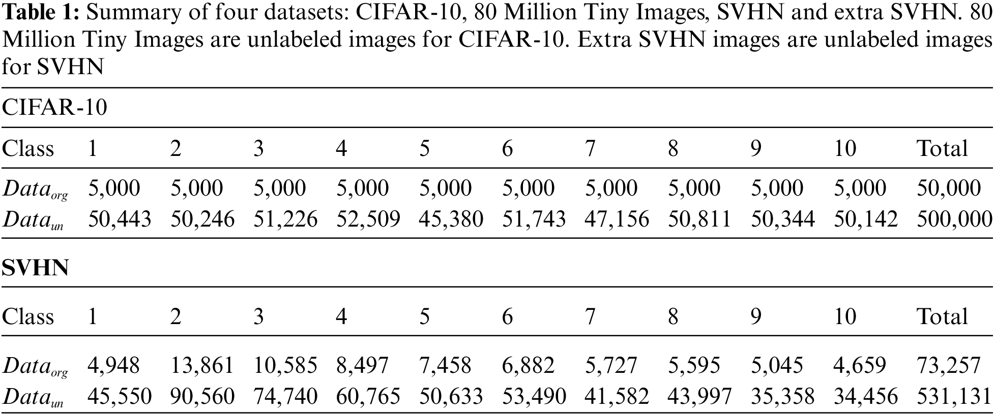
To evaluate our proposed algorithms of ISSL-SP and ISSL-SPR, we mainly used two datasets of CIFAR-10 [31] and the street view house number (SVHN) [32]. The two datasets include images and the corresponding class labels. In addition, they have additional unlabeled data with similar distributions: 80 Million Tiny Images [33] includes the unlabeled images for CIFAR-10, and extra SVHN [32] includes the unlabeled images for SVHN. Tab. 1 summarizes the four datasets of CIFAR-10, 80 Million Tiny Images, SVHN and extra SVHN. More specifically, for training, 80 Million Tiny Images includes 500,000 unlabeled images while CIFAR-10 includes 50,000 labeled images. The extra SVHN includes 531,131 unlabeled images while SVHN includes 73,257 images.

5.2 Experimental Setup

In this study, we conducted experiments on artificially created long-tailed data distribution from CIFAR-10 and SVHN. Tab. 2 summarizes the trained data randomly drawn from datasets of CIFAR-10, 80 Million Tiny Images, SVHN and extra SVHN. The class imbalance ratio was defined as the number of the most frequent class divided by that of the least frequent class [29–31].

For CIFAR-10 and SVHN, we randomly drew samples to make the imbalance ratio of 50, which is denoted by Dataori. For the unlabeled data Dataun, we considered two scenarios with different imbalance ratios. In Scenario 1, we assumed that the unlabeled data was balanced with the imbalance ratio of 1. In Scenario 2, we assumed that the unlabeled data was imbalanced with the imbalance ratio of 50. For both scenarios, we almost balanced out the numbers of labeled and unlabeled data: 13,996 Dataori and 13,990 Dataun from CIFAR-10 and 80 Million Tiny Images while 2,795 Dataori and 2,790 Dataun from SVHN and extra SVHN. Finally, we evaluated each of the trained models on the isolated and balanced testing dataset [30,31,34,35].

We implemented and trained the models using Pytorch. For all experiments, we used the stochastic gradient descent (SGD) optimizer with batch size of 256 and binary cross-entropy for the cost function. The entire experiments were performed on NVIDIA GeForce GTX 1080 Ti GPU.

5.3 Evaluation Metrics

To analyze the performance, the labeling percentage was defined as the number of the labeled data among Dataun divided by the number of Dataun:

Labeledpercentage=n(Dataun′)n(Dataun),(5)

where Dataun′ is with the condition Labelun>0 given Dataun.

To evaluate the performance, we used sensitivity (recall), specificity, precision, accuracy, balanced accuracy (BA) and F1 score as

Sensitivity=recall=TPTP+FN,(6)

precision=TPTP+FP,(7)

Specificity=TNTN+FP,(8)

Accuracy=TP+TNTP+TN+FP+FN,(9)

BalancedAccuracy=Sensitivity+Specificity2,(10)

F1score=2×precision×recallprecision+recall,(11)

where TP, TN, FP, and FN represent the true positive, true negative, false positive, and false negative, respectively. In addition, we also used the metrics of top-1 error.

6  Results

6.1 With Balanced Unlabeled Data: Scenario 1

Tab. 3 summarizes the results when unlabeled data is balanced. It shows sensitivity, specificity, accuracy, BA, F1 score and top-1 error. Note since the testing dataset is balanced, the F1 score can be both macro average and weighted average. For the CIFAR-10 dataset, if only Dataori is used for training as a baseline, the top-1 error is 28.76%. If Dataun is additionally used for training without iteration [30], the top-1 error is 24.93%, which is slightly decreased. On the other hand, if Dataun is ideally given with 100% labeling accuracy and additionally used for training, the top-1 error is significantly dropped to 8.83%, which can be considered the lowest bound. Our proposed algorithms ISSL-SP and ISSL-SPR provide the top-1 error of 14.92% and 10.79%, respectively, which are much lower than that from the method [30], and are very close to the lowest bound. Similarly, for the SVHN dataset, with Dataori only, the top-1 error is 28.10%. If Dataun is additionally used for training without iteration [30], the top-1 error decreases to 25.73%. With the ideal condition using Dataun 100% labeling accuracy, the top-1 error is 9.17% as the lowest bound. Our proposed algorithms ISSL-SP and ISSL-SPR provide the top-1 error of 14.87% and 11.09%, respectively, which are also much lower than that from the method [30], and are very close to the lowest bound. More detailed results are presented in Supplementary Tabs. 1 and 2. In addition, the results show that ISSL-SPR provides slightly higher accuracy than ISSL-SP, indicating that the updated classifier needs to re-label the entire initial unlabeled data.

Fig. 2 plots labeled percentages and top-1 errors using ISSL-SP and ISSL-SPR according to each iteration. It shows that the labeled percentage increases and top-1 error decreases as the labeling processing is repeated. Also, the tendency to change with each iteration can be observed in both algorithms of ISSL-SP and ISSL-SPR.

Figure 2: (Scenario 1: with balanced unlabeled data) Labeled percentages and top-1 errors using ISSL-SP and ISSL-SPR according to each iteration

6.2 With Balanced Unlabeled Data: Scenario 2

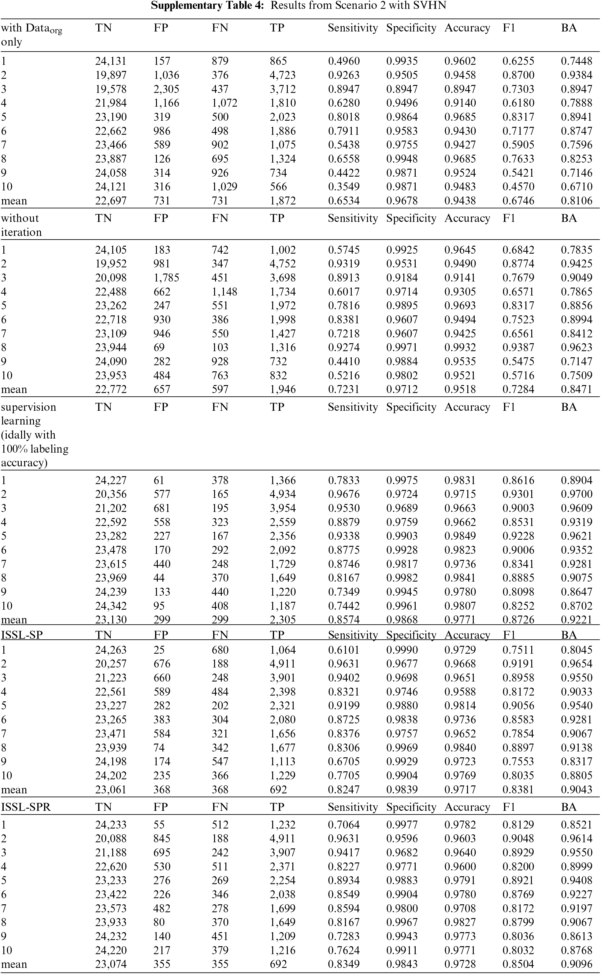
Tab. 4 summarizes the results when unlabeled data is imbalanced. It shows sensitivity, specificity, accuracy, BA, F1 score and top-1 error. For the CIFAR-10 dataset, with Dataori only, the top-1 error is 28.76%. If Dataun is additionally used for training without iteration [30], the top-1 error decreases to 25.85%. As the lowest bound, if Dataun is ideally given with 100% labeling accuracy and additionally used for training, the top-1 error is 11.62%. Our proposed algorithms ISSL-SP and ISSL-SPR provide the top-1 error of 18.58% and 14.87%, respectively, which are also much lower than that from the method [30], and are very close to the lowest bound. Similarly, for the SVHN dataset, with Dataori only, the top-1 error is 28.10%. If Dataun is additionally used for training without iteration [30], the top-1 error decreases to 25.25%. With the ideal condition using Dataun 100% labeling accuracy, the top-1 error is 11.47% as the lowest bound. Our proposed algorithms ISSL-SP and ISSL-SPR provide the top-1 error of 14.14% and 13.62%, respectively, which are also much lower than that from the method [30], and are very close to the lowest bound. More detailed results are presented in Supplementary Tabs. 3 and 4. In addition, similar to the scenario 1, the results show that ISSL-SPR provides slightly higher accuracy than ISSL-SP, indicating that the updated classifier needs to re-label the entire initial unlabeled data.

Fig. 3 plots labeled percentages and top-1 errors using ISSL-SP and ISSL-SPR according to each iteration. It also shows that the labeled percentage increases and top-1 error decreases as the labeling processing is repeated.

Figure 3: (Scenario 2: with balanced unlabeled data) Labeled percentages and top-1 errors using ISSL-SP and ISSL-SPR according to each iteration

6.3 Effect of Softmax Threshold Values

To investigate the effect of the softmax threshold values, we changed the threshold values from 0.5 to 0.999: by the increment of 0.01 from 0.5 to 0.9, and the increment of 0.001 from 0.9 to 0.999. Fig. 4 shows the accuracy metrics of F1 score, balanced accuracy and top-1 error according to the softmax threshold values. The results show that the threshold value of 0.99 provides the highest accuracy values. Throughout this study, we have used the softmax threshold value of 0.99 for the simulation results.

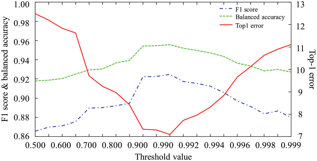
Figure 4: F1 score, Balanced accuracy and top-1 errors according to softmax threshold values

7  Conclusion and Discussion

In this study, we propose new semi-supervised learning algorithms, which iteratively corrects the labeling of the extra unlabeled data based on softmax probabilities. We first train a base classifier using original labeled data, and evaluate unlabeled data using softmax probabilities. For each unlabeled data, if the maximum value of the softmax probabilities is equal or greater than 0.99, we assign the unlabeled data with the corresponding class. Every iteration, we update the classifier using all available data for training. Regarding the labeling, ISSL-SP considers only the remaining unlabeled data while ISSL-SPR considers the entire initial unlabeled data. To validate the proposed algorithms, we tested on the two scenarios: with balanced unlabeled dataset and with imbalanced unlabeled dataset. The results show that the two proposed algorithms, ISSL-SP and ISSL-SPR, provide the accuracy as high as that from supervised learning, where the unlabeled data is given 100% labeling accuracy.

Comparing the performance of the two algorithms of ISSP-SP and ISSP-SPR, ISS-SPR outperforms ISS-SP regardless of the datasets and the imbalance ratio of unlabeled data. The results indicate that the updated classifier needs to re-label the entire initial unlabeled data. Furthermore, ISS-SPR outperforms previous state-of-the-arts. In the future work, we plan to validate the algorithm efficacy using more extended datasets. In addition, we need to investigate an optimum strategy to reduce the lengthy training time caused by the iteration process.

Funding Statement: This work was supported by the National Research Foundation of Korea (No. 2020R1A2C1014829), and by the Korea Medical Device Development Fund grant, which is funded by the Government of the Republic of Korea Korea government (the Ministry of Science and ICT; the Ministry of Trade, Industry and Energy; the Ministry of Health and Welfare; and the Ministry of Food and Drug Safety) (grant KMDF_PR_20200901_0095).

Conflicts of Interest: The authors declare that they have no conflicts of interest to report regarding the present study.

References

 1.  S. S. Nath, G. Mishra, J. Kar, S. Chakraborty and N. Dey, “A survey of image classification methods and techniques,” in 2014 Int. Conf. on Control, Instrumentation, Communication and Computational Technologies (ICCICCT), Kanyakumari District, India, pp. 554–557, 2014. [Google Scholar]

 2.  E. Miranda, M. Aryuni and E. Irwansyah, “A survey of medical image classification techniques,” in 2016 Int. Conf. on Information Management and Technology (ICIMTech), Bandung, Indonesia, pp. 56–61, 2016. [Google Scholar]

 3.  E. Vocaturo, “Image classification techniques,” in Handbook of Research on Disease Prediction Through Data Analytics and Machine Learning, Pennsylvania, USA, pp. 22–49. IGI Global, 2021. [Google Scholar]

 4.  S. Shakya, “Analysis of artificial intelligence based image classification techniques,” Journal of Innovative Image Processing (JIIP), vol. 2, no. 1, pp. 44–54, 2020. [Google Scholar]

 5.  W. Sun, G. Dai, X. Zhang, X. He and X. Chen, “TBE-Net: A three-branch embedding network with part-aware ability and feature complementary learning for vehicle re-identification,” IEEE Transactions on Intelligent Transportation Systems, pp. 1–13, 2021. DOI 10.1109/TITS.2021.3130403. [Google Scholar] [CrossRef]

 6.  W. Sun, L. Dai, X. Zhang, P. Chang and X. He, “RSOD: Real-time small object detection algorithm in UAV-based traffic monitoring,” Applied Intelligence, vol. 92, no. 6, pp. 1–16, 2021. [Google Scholar]

 7.  A. Krizhevsky, I. Sutskever and G. E. Hinton, “Imagenet classification with deep convolutional neural networks,” Advances in Neural Information Processing Systems, vol. 25, pp. 1097–1105, 2012. [Google Scholar]

 8.  K. Simonyan and A. Zisserman, “Very deep convolutional networks for large-scale image recognition,” 2014. [Online]. Available: https://arxiv.org/abs/1409.1556. [Google Scholar]

 9.  C. Szegedy, W. Liu, Y. Jia, P. Sermanet, S. Reed et al., “Going deeper with convolutions,” in Proc. of the IEEE Conf. on computer vision and pattern recognition, Boston, MA, USA, pp. 1–9, 2015. [Google Scholar]

10. K. He, X. Zhang, S. Ren and J. Sun, “Deep residual learning for image recognition,” in Proc. of the IEEE Conf. on computer vision and pattern recognition, Las Vegas, NV, USA, pp. 770–778, 2016. [Google Scholar]

11. C. Szegedy, V. Vanhoucke, S. Ioffe, J. Shlens and Z. Wojna, “Rethinking the inception architecture for computer vision,” in Proc. of the IEEE Conf. on Computer Vision and Pattern Recognition, Las Vegas, NV, USA, pp. 2818–2826, 2016. [Google Scholar]

12. J. M. Overhage and D. McCallie Jr, “Physician time spent using the electronic health record during outpatient encounters: A descriptive study,” Annals of Internal Medicine, vol. 172, no. 3, pp. 169–174, 2020. [Google Scholar]

13. M. J. Willemink, W. A. Koszek, C. Hardell, J. Wu, D. Fleischmann et al., “Preparing medical imaging data for machine learning,” Radiology, vol. 295, no. 1, pp. 4–15, 2020. [Google Scholar]

14. Y. Xu, T. Mo, Q. Feng, P. Zhong, M. Lai et al., “Deep learning of feature representation with multiple instance learning for medical image analysis,” in 2014 IEEE Int. Conf. on Acoustics, Speech and Signal Processing, Florence, Italy, pp. 1626–1630, 2014. [Google Scholar]

15. J. E. Van Engelen and H. H. Hoos, “A survey on semi-supervised learning,” Machine Learning, vol. 109, no. 2, pp. 373–440, 2020. [Google Scholar]

16. T. Miyato, S.-i Maeda, M. Koyama and S. Ishii, “Virtual adversarial training: A regularization method for supervised and semi-supervised learning,” IEEE Transactions on Pattern Analysis and Machine Intelligence, vol. 41, no. 8, pp. 1979–1993, 2018. [Google Scholar]

17. W. Bai, O. Oktay, M. Sinclair, H. Suzuki, M. Rajchl et al., “Semi-supervised learning for network-based cardiac MR image segmentation,” in Int. Conf. on Medical Image Computing and Computer-Assisted Intervention, Quebec City, Quebec, Canada, pp. 253–260, 2017. [Google Scholar]

18. B. Krawczyk, “Learning from imbalanced data: Open challenges and future directions,” Progress in Artificial Intelligence, vol. 5, no. 4, pp. 221–232, 2016. [Google Scholar]

19. H. Kaur, H. S. Pannu and A. K. Malhi, “A systematic review on imbalanced data challenges in machine learning: Applications and solutions,” ACM Computing Surveys, vol. 52, no. 4, pp. 1–36, 2019. [Google Scholar]

20. G. H. Nguyen, A. Bouzerdoum and S. L. Phung, “Learning pattern classification tasks with imbalanced data sets,” Pattern Recognition, pp. 193–208, 2009. [Online]. Available: https://ro.uow.edu.au/infopapers/792/. [Google Scholar]

21. Y. Yan, M. Chen, M.-L. Shyu and S.-C. Chen, “Deep learning for imbalanced multimedia data classification,” in 2015 IEEE International Symposium on Multimedia (ISM), Miami, FL, USA, pp. 483–488, 2015. [Google Scholar]

22. Y. Yan, M. Chen, M.-L. Shyu and S.-C. Chen, “Deep learning for imbalanced multimedia data classification,” in 2015 IEEE International Symposium on Multimedia (ISM), Miami, FL, USA, pp. 483–488, 2015. [Google Scholar]

23. N. V. Chawla, N. Japkowicz and A. Kotcz, “Special issue on learning from imbalanced data sets,” ACM SIGKDD Explorations Newsletter, vol. 6, no. 1, pp. 1–6, 2004. [Google Scholar]

24. J. M. Johnson and T. M. Khoshgoftaar, “Survey on deep learning with class imbalance,” Journal of Big Data, vol. 6, no. 1, pp. 1–54, 2019. [Google Scholar]

25. N. V. Chawla, K. W. Bowyer, L. O. Hall and W. P. Kegelmeyer, “SMOTE: Synthetic minority over-sampling technique,” Journal of Artificial Intelligence Research, vol. 16, pp. 321–357, 2002. [Google Scholar]

26. H. He, Y. Bai, E. A. Garcia and S. Li, “ADASYN: Adaptive synthetic sampling approach for imbalanced learning,” in 2008 IEEE Int. Joint Conf. on Neural Networks (IEEE World Congress on Computational Intelligence), Hong Kong, China, pp. 1322–1328, 2008. [Google Scholar]

27. C. Elkan, “The foundations of cost-sensitive learning,” in Int. Joint Conf. on Artificial Intelligence, Seattle, Washington, USA, pp. 973–978, 2001. [Google Scholar]

28. C. X. Ling and V. S. Sheng, “Cost-sensitive learning and the class imbalance problem,” Encyclopedia of Machine Learning, vol. 2011, pp. 231–235, 2008. [Google Scholar]

29. Y. Cui, M. Jia, T.-Y. Lin, Y. Song and S. Belongie, “Class-balanced loss based on effective number of samples,” in Proc. of the IEEE/CVF Conf. on computer vision and pattern recognition, Long Beach, CA, USA, pp. 9268–9277, 2019. [Google Scholar]

30. Y. Yang and Z. Xu, “Rethinking the value of labels for improving class-imbalanced learning,” 2020. [Online]. Available: https://arxiv.org/abs/2006.07529. [Google Scholar]

31. K. Cao, C. Wei, A. Gaidon, N. Arechiga and T. Ma, “Learning imbalanced datasets with label-distribution-aware margin loss,” 2019. [Online]. Available: https://arxiv.org/abs/1906.07413. [Google Scholar]

32. Y. Netzer, T. Wang, A. Coates, A. Bissacco, B. Wu et al., “Reading digits in natural images with unsupervised feature learning,” in NIPS Workshop, Granada, Spain, 2011. [Google Scholar]

33. A. Torralba, R. Fergus and W. T. Freeman, “80 Million tiny images: A large data set for nonparametric object and scene recognition,” IEEE Transactions on Pattern Analysis and Machine Intelligence, vol. 30, no. 11, pp. 1958–1970, 2008. [Google Scholar]

34. B. Kang, S. Xie, M. Rohrbach, Z. Yan, A. Gordo et al., “Decoupling representation and classifier for long-tailed recognition,” 2019. [Online]. Available: https://arxiv.org/abs/1910.09217. [Google Scholar]

35. Z. Liu, Z. Miao, X. Zhan, J. Wang, B. Gong et al., “Large-scale long-tailed recognition in an open world,” in Proc. of the IEEE/CVF Conf. on Computer Vision and Pattern Recognition, Long Beach, CA, USA, pp. 2537–2546, 2019. [Google Scholar]

36. S. Laine and T. Aila, “Temporal ensembling for semi-supervised learning,” 2016. [Online]. Available: https://arxiv.org/abs/1610.02242. [Google Scholar]

37. A. Tarvainen and H. Valpola, “Weight-averaged consistency targets improve semi-supervised deep learning results,” CoRR, 2017. [Online]. Available: https://arxiv.org/abs/1703.01780. [Google Scholar]

38. V. Verma, K. Kawaguchi, A. Lamb, J. Kannala, Y. Bengio et al., “Interpolation consistency training for semi-supervised learning,” 2019. [Online]. Available: https://arxiv.org/abs/1903.03825. [Google Scholar]

39. K. Sohn, D. Berthelot, C.-L. Li, Z. Zhang, N. Carlini et al., “Fixmatch: Simplifying semi-supervised learning with consistency and confidence,” 2020. [Online]. Available: https://arxiv.org/abs/2001.07685. [Google Scholar]

This work is licensed under a Creative Commons Attribution 4.0 International License, which permits unrestricted use, distribution, and reproduction in any medium, provided the original work is properly cited.