DOI:10.32604/cmc.2022.028512
| Computers, Materials & Continua DOI:10.32604/cmc.2022.028512 | |
| Article |
ENSOCOM: Ensemble of Multi-Output Neural Network’s Components for Multi-Label Classification
Department of Information Systems, Al-Qunfudhah Computing College, Umm Al-Qura University, Al-Qunfudhah, Mecca, Saudi Arabia
*Corresponding Author: Khudran M. Alzhrani. Email: kmzhrani@uqu.edu.sa
Received: 11 February 2022; Accepted: 18 March 2022
Abstract: Multitasking and multioutput neural networks models jointly learn related classification tasks from a shared structure. Hard parameters sharing is a multitasking approach that shares hidden layers between multiple task-specific outputs. The output layers’ weights are essential in transforming aggregated neurons outputs into tasks labels. This paper redirects the multioutput network research to prove that the ensemble of output layers prediction can improve network performance in classifying multi-label classification tasks. The network’s output layers initialized with different weights simulate multiple semi-independent classifiers that can make non-identical label sets predictions for the same instance. The ensemble of a multi-output neural network that learns to classify the same multi-label classification task per output layer can outperform an individual output layer neural network. We propose an ensemble strategy of output layers components in the multi-output neural network for multi-label classification (ENSOCOM). The baseline and proposed models are selected based on the size of the hidden layer and the number of output layers to evaluate the proposed method comprehensively. The ENSOCOM method improved the performance of the neural networks on five different multi-label datasets based on several evaluation metrics. The methods presented in this work can substitute the standard labels representation and predictions generation of any neural network.
Keywords: Ensemble learning; multilabel classification; neural networks
Accelerating advances in intelligent computer modeling promoted their adoption as solutions to complex tasks. Classification problems that traditional single and multiclass intelligent models cannot address are handled with task-oriented learning techniques. In classification tasks, the ensemble methods are often referred to as multiple classifier systems that combine the prediction of the multiple learners to improve performance and robustness. One clear advantage of the multiple classifiers systems over the individual classifier is reducing the variance [1], which improves the collection of models’ predictive accuracy.
Ensemble learning is considered homogeneous when all the base classifiers are of the same type; neural network ensemble only consists of neural networks. Homogeneous ensemble learning methods can be categorized into two general categories known as bagging and boosting. The classifiers in Bagging methods learn in parallel, whereas the boosting methods classifier learns sequentially. The classifiers’ predictions are combined based on a fusion strategy. However, the current neural networks ensemble methods require building multiple neural network models. In practice, compiling and running the multiple neural network models is often sequential.
Neural networks architecture is adjustable and can be modified depending on classification tasks and datasets. The flexibility of deep neural networks enabled researchers to design novel architectures suited for a wide range of classification applications. Multi-output neural networks provide the ability to perform multiple tasks simultaneously [2]. The need for models that maps between a single input to multiple outputs is emerging in many fields [3,4]. The outputs might represent various tasks or data types [5]. Multi-label classification is one of the domains that benefited from multioutput neural networks [6].
Unlike multiclass and single classification, instances in multi-label classification can be labeled with one or more classes. The Input features are mapped to a non-fixed number of overlapping classes for each instance, making the learning process more complicated. Assuming the input space is represented by X, which are instances of the multi-label dataset D. The attributes extracted from the dataset D are denoted as A, and all possible labels for D instances X as L. Moreover, the output space is represented as Y. Hence, the dataset instances and attributes association is represented as
This work combines three concepts, multi-label, multioutput, and ensemble learning, to construct and improve the performance of a neural network. Each output layer is dedicated to predicting a single class label in the conventional multioutput neural network for multi-label classification. We extend the traditional approaches of classifying multi-label data in neural networks by restructuring the label representation in the output layers. Output layer-based classifiers create multiple end paths within the neural network with different initialized weights and backpropagation. Therefore, the proposed method can make multiple predictions using a single neural network for the same instance. Other neural network ensemble methods require several neural networks to be built and run separately. We are unaware of previous studies that utilized a single neural network to learn different outcomes for the same output. The purpose of this work is to test the ability of the ENSOCOM method to outperform the results of a neural network for multi-label classification. In order to limit the influence of the neural networks factors on the models’ outcomes, a shallow multilayer perceptron (MLP) is used for the baseline and ENSOCOM models. However, the proposed methodology can extend any neural network by restructuring its final layer. The construction of this paper is summarized as follows:
• We developed a methodology to construct multiple classifiers from a single multi-output neural network. The set of classifiers can be trained simultaneously without recompiling.
• We designed a strategy to select the best model for each output-based classifier in the neural network.
• We introduced an ensembling method that mitigates the effect of data imbalance in multi-label classification.
• The proposed models outperformed the baselines in multi-label classification problems based on several evaluation metrics.
The rest of the paper is organized as follows: In Section 2, works related to the ensemble of multi-label classification are briefly discussed and reviewed. Details on the design and specifications of the proposed work are presented in Section 3. Statistical information and a brief review of the datasets are listed in Section 4. In Section 5, experiments and results are illustrated to evaluate the performance of the proposed method. The future work and conclusions of the paper are discussed in Section 6.
Problem transformation learning techniques reduce multi-label classification complexity by converting labels to a more straightforward form. Binary Relevance (BR) is one of the earliest transformation methods that assign a classifier to each label [7,8]. In traditional supervised learning settings, classifiers learn to map between a feature set and a class or an object, as in text [9,10], and image classification problems [11] or object detection [12], which is often represented by a single exclusive label for each instance. For multi-label problems, BR imitates the traditional approaches by assigning a classifier for each label that predicts the label’s presence or absence for all unseen examples. One of the drawbacks of BR is the lack of correlation among instance labels, which might influence the models’ prediction performance [13]. Therefore, multiple research papers proposed an extension to BR that includes label correlation in the learning process. One of the most popular approaches to provide correlation capabilities to BR methods is Classifiers Chain (CC) [14,15]. CC technique builds a chain of classifiers that predict single label association to an instance via passing the classifier’s feature space to the following one. Sharing the feature space to the subsequent classifier mitigates label independence issues in the traditional BR method. However, CC performance is highly susceptible to the order of classifiers in the chain because label information sharing occurs between adjacent classifiers. One way to improve CC is by Ensemble Classifier Chains (ECC), which sums the votes generated by a randomly structured CC to limit the effect of classifiers’ order in the chains.
Label Powerset (LP) is another approach that reduces data labels entanglement and enables the correlation of multi-label data by combining the associated set of labels into a single atomic label [16,17]. The combination of labels allows for treating the multi-label problem as a standard multiclass classification. Since every unique combination of labels is considered a single label, as a result, there might be many newly constructed classes. The number of classes will vary depending on the dataset. One can train the classifier on the most relevant labels by pruning the less important ones [18].
On the other hand, some learning approaches adapted to the multi-label problem by extending the existing algorithm that worked with the standard multiclassification task to a suitable one. For instance, a variation of the K-nearest neighbor algorithm (ML-KNN) [19] determines the training set’s K-nearest neighbors. The maximum a posteriori (MAP) principle identifies labels associated with each unseen instance based on statistical information obtained from neighbors’ label sets. Similarly, a well-known algorithm for multiclass classification, decision trees effectively predict hierarchal multi-label instances without label transformation [20]. Labels in hierarchal multi-label data [21] are structured to organize the label set associated with an instance into parents and children labels, assuming label dependency. Some other approaches rely on optimizing classifiers, such as SVM, to better fit algorithm parameters on multi-label data by using a label ranking method based on a cost function [22].
Customizability is one of the deep neural networks features that provided solutions to a diverse multi-label application. Deep neural networks are apt to implement problem transformation and adaptation techniques. A learning network with a single RNN layer was trained to predict the labels of several multi-label datasets [23]. The experiment showed that the adapted version of the neural network outperformed several multi-label learning techniques, including a variation of the RNN network that implemented the classifiers chain method.
A shallow Multilayer Perceptron with a single layer and a deep one with two layers was trained on patients’ examination records to detect chronic diseases, such as diabetes and hypertension [24]. The records are labeled with zero or more diseases totaling eight unique classes. The authors used several traditional classifiers and the multilayer perceptron network to learn from the original multi-label sets and the unique set (LP). The paper showed that the deep neural networks reported higher accuracy than other classifiers but lower F1-score on multi-label sets. Bidirectional RNN with attention mechanism neural networks was employed to predict the labels of three biomedical text datasets in [25]. The proposed framework had two outputs, one for the number of labels associated with the instance and the second for the labels set. The authors claimed that their proposed method is favorable compared to other deep neural network frameworks and BR. Besides emphasizing the neural networks themselves, the Hierarchical Label Set Expansion method introduced in [26] added more complexity to the multi-label data by expanding the label sets. The approach is suitable for hierarchal multi-label datasets since it finds missing labels between descendants and ancestors to append to the labels set.
Due to the difficulty in handling multi-label classification problems, the ensembled methods that use deep neural networks are considered promising solutions. For example, the ensemble of classifiers for multi-label classification has applications in video object recognition. One proposed using the ensemble of two deep neural networks, GoogleLeNet and VGGNet, to detect surgical tools in laparoscopic videos [27]. Before learning the network, the surgical tools labels were combined into a single label. The two neural networks’ outputs were averaged to compute the final prediction. The ensemble method outperforms the paper’s other baselines based on the mean accuracy precision metric.
The use of the ensemble of five different neural network frameworks to predict tweets’ labels is presented in [28]. The comparison was made between two ensemble approaches, namely stacked and weighted. A stacked ensemble of the five classifiers was conducted by concatenating the output of all models before passing it into two fully connected layers. The weighted ensemble sums the product of a tensor, the neural networks models output, over a single axis to construct a one-dimensional vector representing a tweet’s labels. The paper reported that the weighted ensemble approach performed slightly better than the stacked one.
3.1 Single and Multi-Output Deep Neural Networks
Changes are made to the conventional DNN structure to adapt to MLC problems that expect each sample in the dataset to be marked with one or more labels. As seen in Fig. 1, two general approaches represent multiple labels at the network’s end. The first approach is to approximate the problem of MLC in DNN by creating multiple output layers equal to the number of all possible labels of a dataset. In the standard multioutput neural network for MLC, each output layer has a single neuron that takes the inputs from the proceeding layer. The neuron sums the dot product of inputs and their corresponding weights, which is often computed by matrix manipulation.
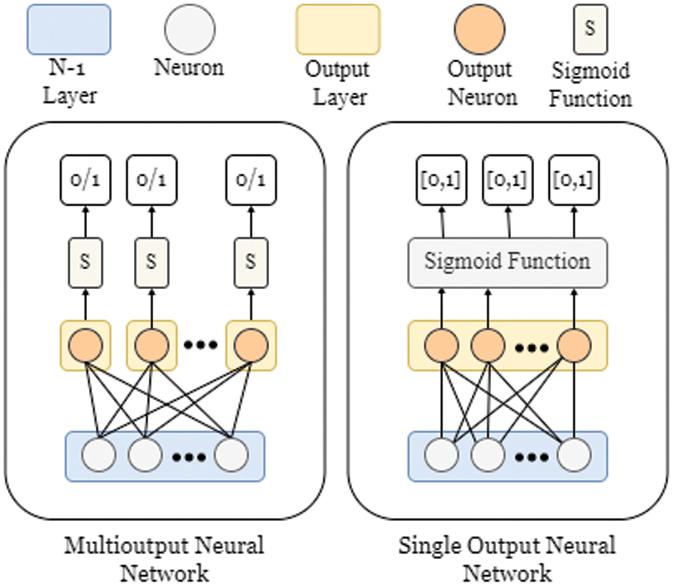
Figure 1: Single vs. multi-output neural networks for multilabel classification
In most cases, the weights in the network layers are trainable to determine the influence or importance of input values of the neurons. Classes are exclusive in binary and multiclass classification problems so that any given instance will be labeled with one class. Every output layer in the standard multioutput neural networks for MLC acts similarly to the output layer of a single classification network. The outcomes returned by the output layers’ neurons are separately passed into an activation function.
The activation function produces a score representing confidence degree that predicts the label presence or absence in an instance. In other words, the expected output of the activation function after thresholding is either 0 or 1. The simplest thresholding method is scaling down values less than 0.5 to 0 and higher ones to 1. Sigmoid function has this property that squash neurons output to produce a floating-point number. However, it is worth noting that there is another way to conduct binary classification problems in DNN. It is possible to perform binary classification problems with two neurons in the output layer instead of one.
The Sigmoid function will not be appropriate for standard multiple-output networks with two neurons in the output layer. It can be done by a well-known activation function that measures the probability of a class belonging to an instance, namely SoftMax. Each output layer passes its outcome to the SoftMax function that produces a probability distribution over all the possible classes. The sum of the probability distribution generated by the SoftMax activation function equals 1. The class that received the highest probability among the output components is designated as the prediction of that output. The SoftMax function for binary and multiclass classification is mathematically defined as follows:
However, assigning a separate output layer for each unique class is challenging to manage. The second approach that DNN can take to perform MLC tasks, Fig. 1, is by limiting the number of outputs in the DNN to a single output layer with multiple neurons equal to the number of unique labels in the dataset. Correspondingly, the output layer has a single vector with multiple components that allocates all possible classes. This approach requires an activation function that measures the degree of confidence for every class independently. The sigmoid activation function is known by its ability to produce a score for all the possible labels with values ranging between 0 and 1 independently. The sigmoid function is defined as:
The main difference between the multioutput and single output DNN for multi-label classification is that the loss is optimized over each output layer in the multi-output neural network, one output layer per class. While in a single output layer neural network, the loss optimization is done for each output component, one class per component. Nonetheless, both are valid approaches and are widely used in practice.
3.2 Ensemble of Output Components in Multioutput Neural Network
This paper proposes another approach that takes advantage of DNN flexibility in specifying the number of output layers. The ensemble of outputs’ components of multioutput neural networks (ENSOCOM) combines some properties of the single output and multi-output neural network for MLC to improve its performance. Before going into the details of the ENSOCOM framework, we will briefly highlight the learning process of DNN.
Deep Neural networks are a collection of neurons organized and grouped in multiple layers. A neural network with a single hidden layer is often referred to as a shallow neural network. In multiple layers neural networks, upper layers are often used to extract features from the dataset, and the lower ones are fully connected layers. All neurons or nodes are connected to the preceding and posterior layers in the fully-connected networks, hence the name. Neurons aggregate the incoming connections from the previous layer and apply an activation function. Several well-documented activation functions in the literature for intermediate layers improve the network’s ability to learn complex patterns. The connections between neurons edges and bias vector are the learnable parameters of neural networks, also known as weights W. These weights are updated in the training phase to map input space attributes to a label or a subset of all possible labels. The connection between two layers can be mathematically defined as follows:
where
The final layer in the network is an output layer that makes predictions based on all learnable parameters’ values. The network’s performance is measured by a cost function that considers neural network weights W, biases B, the input of an instance
The cost of function for predicting a training instance is used to find the error of the output layer δ as in the following equation:
In backpropagation, the weights are updated according to a gradient descent optimizer to minimize the error of the cost function. Therefore, a gradient measures the relationship between changes made to the network weights concerning the network error.
The initialized weights are essential in network optimization since they are considered the starting point for reaching the global optimum [29]. Although the weights are initialized before the actual learning starts, it impacts the final outputs of the network. Therefore, several weights initialization mechanisms can be seen in the literature. Zero initialization is one of the simplest initialization methods, where all weights are set to zeros. However, initializing weights with zeros will result in layers receiving the exact update and preventing the network from learning different functions at each neuron. Initializing weights with different values will break the symmetry of neurons located in the same layer with identical inputs and activation functions. While there are multiple weights initialization approaches, we are interested in weights initialized from a random distribution.
As with any layer, the output layer of the deep neural network also has trainable weights. The output layer weights are the first to be updated in the backpropagation phase. Fig. 2 illustrates the lower end of the network of the proposed framework that ensembles the multi-output neural network’s output components (ENSOCOM).
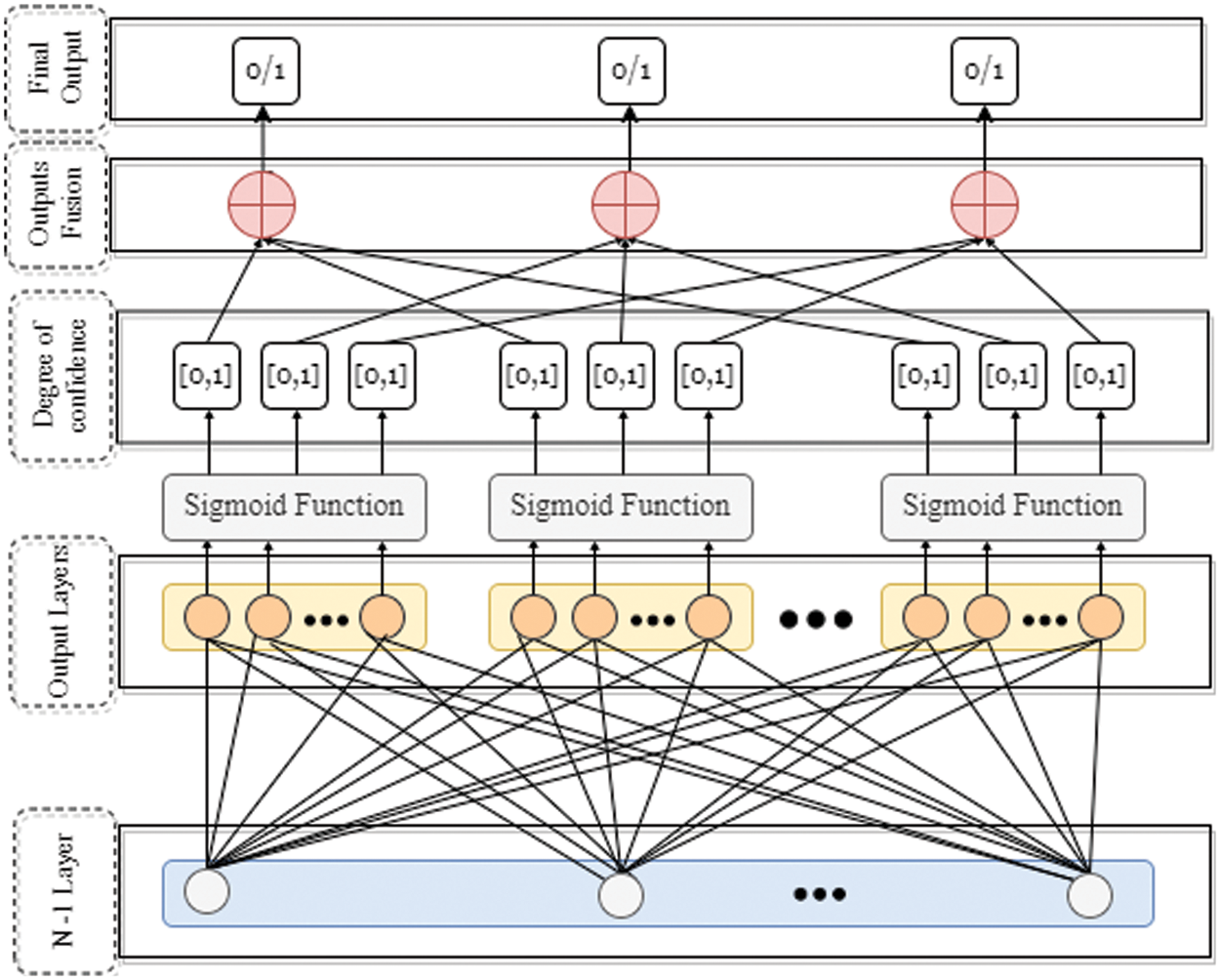
Figure 2: Ensemble of output layers components
ENSOCOM is a neural network with a multioutput layer. Each one of the output layers has the same number of neurons that represent classes in the multi-label set. The output layers are identical regarding their inputs, activation functions, and expected outputs. However, the weights for all output layers are initialized separately and are not the same. Hence, the output layers will have distinct predictions and costs in the first iteration of the forward propagation. Since the updates made to the output layers differ depending on their cost function, the starting point for finding the global optimum is not identical for the output layers. The more the network is updated in every iteration, the closer each output layer gets to the global optimum. Because the output layers are initialized with different weights, their outcomes will differ. We argue that ENSOCOM will search for different paths to minimize the error for each output layer, resulting in learning more patterns.
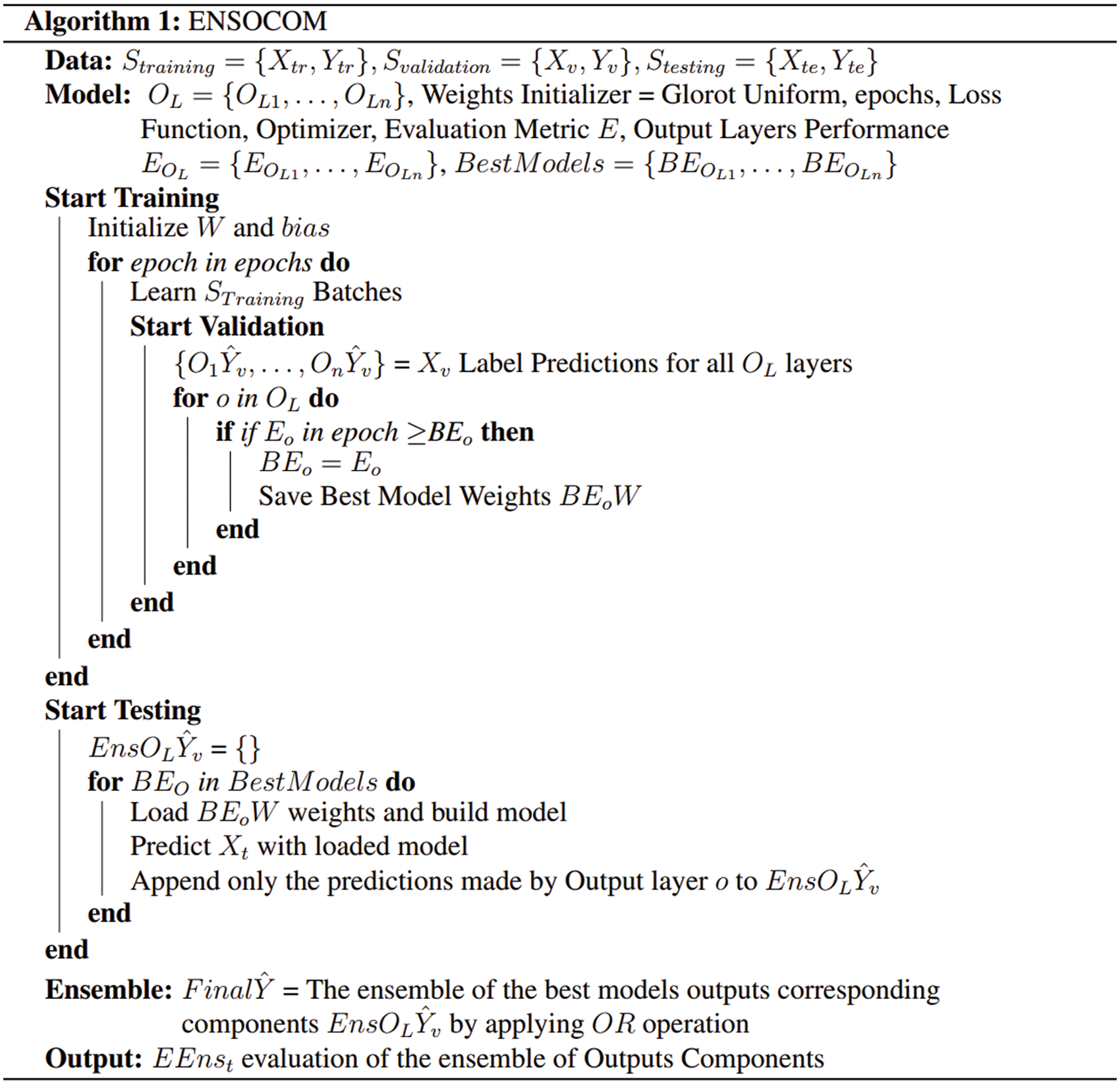
ENSOCOM enables the network to make multiple predictions for the same class without constructing additional networks. Since the output layers in ENSOCOM makes predictions regarding all the possible labels in a component set, the Sigmoid function is employed in each output layer. The Sigmoid function will take inputs and independently produce a confidence degree for each component in the output layer. As we have said before, the predictions made for each corresponding component across output layers are not necessarily the same. In other words, ENSOCOM constructs multiple prediction models, which share the same input and hidden layer from a single neural network. Pseudocode 1 illustrates the entirety of the proposed ENSOCOM methodology.
The neural network will iterate over training examples during the training phase to improve the network accuracy and minimize the error rate. Network performance on the training set is not a good indicator of the model’s ability to accurately predict unseen data’s label. After each epoch, the model is evaluated on unseen examples, also known as a validation set. In single output layer neural networks, the model that performed the best on the validation set is often selected for evaluation on the testing set. The same concept can be applied to multioutput neural networks by choosing the best-performed model on the validation set for every output layer. The weights of the prediction model will be saved if the output layer performance on the validation set on the current epoch is better than the previous ones. The best model selection process is independent and only considers the accuracy of a single output layer at the time. A group of best-fitted models on the validation set will be created by the end of the training phase. It is worth mentioning that the best models for the output layers do not have to be from the same epoch. In other words, the model weights will be saved for every output layer separately regardless of the epoch. The final number of models saved weights equals the number of output layers in the neural network. The best model-saved weights are associated with the corresponding output, and they will be used later in the testing phase.
In the testing phase, one can loop through the models’ saved weights and load them to the neural network architecture. As seen in Algorithm1, each output layer is considered an independent classifier for classifying multi-labeled instances. The saved weights associated with the output layer are loaded to the neural network. The entire network, including all the output layers, is set with the saved weights to predict the instances in the testing set. The predictions made with the output layer associated with the saved weights are used in the ensemble phase; predictions made by the other output layers are discarded. The exact process is repeated for all the output layers (classifiers). The outcome of the whole procedure is a multidimensional array of predictions made by the classifiers. The size of the multidimensional array is (
Now that we have multiple prediction sets for the same class per instance, we must determine the final prediction set. Labels in classification problems are represented as predefined values known as categorical or nominal data. The categorical data could be strings or integer numbers, limiting the learning process. The number of classes is not identical for all instances in the multi-label classification. However, having different number label sets for each instance raises some implementation difficulties. Therefore, the label sets for every instance are represented by a binary vector that indicates a label’s presence and absence. The collection of label sets associated with all instances in the dataset is a
The multidimensional array that consists of all predictions made by the best model per output layer is used in the ensemble process. Fig. 3 shows a snapshot of the ensemble process for a single instance, where multiple predictions are transformed into binary vectors form. Each component in the output layers vector is converted to a 0 or 1. Bitwise OR operation is applied on all the corresponding components generated by the output-based models. This strategy focuses on capturing the positive labels predicted by the model while ignoring the negative ones. One clear advantage of this approach is limiting the data imbalance problem in multi-label classification by giving labels with low representation in the dataset a better chance of getting detected. Also, the more significant is the number of the output layers (classifiers), the higher are the chances that some output-based models might detect patterns not seen by the other models. Of course, one clear drawback of this fusion technique is increasing the false positive rate.
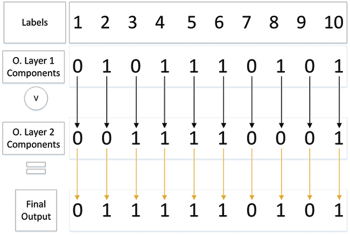
Figure 3: Fusion of multiple predictions by OR operation for a multilabel instance
Five datasets are selected from various domains to represent multi-label classification problems better. The datasets are well-cited standardized with stratified training and testing sets. The domains covered in the datasets are domains texts, biology, and images, as shown in Tab. 1. The Table shows several statistics concerning the selected dataset, such as instances and labels numbers. All the datasets discussed and experimented on in this paper were initially published on MULAN [30], an open-source data repository that supports java learning from multi-label datasets.
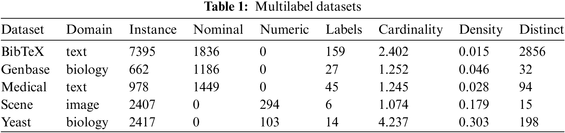
The models’ performance of the multi-label classification tasks can be measured in accuracy and speed. Therefore, the Scikit-multilearn repository introduced Python compatibility for easier access and manipulation. A more significant number of instances provides classifiers with more information that can help to identify patterns between the feature space and the labels. Nominal attributes often represent names or categories related to the instance. Zipcodes, gender, or hair color are examples of nominal attributes. The numerical attributes in the datasets have values that can be measured. One can assume that the larger is the number of the labels, the more difficult it is to find all labels associated with an instance. Cardinality is another information in the dataset statistics table that indicates the average number of labels per instance. In addition, density is measured by dividing cardinality by the number of labels. Finally, distinct is the number of unique labels combination in the dataset.
The datasets are generalized, meaning all features are already extracted and ready for training without preprocessing. The following is a brief description of each one of the datasets. BibTeX [31] is one of the most recognized text datasets for multi-label classification. An instance in a BibTeX contains bibliography items associated with articles, books, or thesis. The BibTeX dataset was constructed by collecting items tagged in users’ submissions to Bibsonomy, a publication sharing system. The main application of the BibTeX dataset is to support a recommender system that automatically identifies tags of unseen BibTeX instances. Tab. 1 shows that BibTeX has the highest number of labels, distinct label sets, and features compared to other datasets.
The second dataset, Genbase [32], belongs to the biology domain, which contains protein sequences with classes representing protein families. The protein sequence can belong to one or more protein family classes. It has the lowest number of instances and features among the other multi-label classification datasets. On the other hand, the Medical dataset [33] is anonymized clinical text collected from Cincinnati Children’s Hospital Medical Center’s Department of Radiology. The clinical texts represent radiology reports that include ICD-9-CM codes assignments that indicate clinical history and radiologists’ impressions. Except for the Genbase dataset, the Medical dataset has fewer instances than the other three but has a relatively high number of features and labels.
In addition to the previous datasets, the Scene dataset [34] includes natural scenes images labeled with classes such as beach and sunset. The Scene dataset has the lowest number of multi-label and distinct label sets. Finally, the Yeast dataset [22] is constructed by micro-array expression data and phylogenetic profiles representing the gene set. Functionality classes, such as metabolism, and aging, are assigned for each yeast gene. As shown in Tab. 1, genes can be associated with many functionality classes, resulting in high cardinality and density values.
5.1 Neural Network Architectures and Experiments Setup
Deep neural networks are categorized into multiple types based on their architectures and tasks. The dominant types of DNN are Convolutional Neural Networks (CNN), Recurrent Neural Networks (RNN), and Artificial Neural Networks (ANN), also known as FeedForward Neural Networks. CNN is suited for features engineering and extraction from images, texts, and audio. On the other hand, RNN is often associated with learning that requires time series or specific sequenced data. Multilayer Perceptron (MLP) are purely made by fully-connected layers, a special class of FeedForward Neural Networks. Fully-connected layers are the building blocks of MLP, and they are placed at the lower end of CNN and RNN. The multi-label datasets we are experimenting on are generalized and standardized for competitive benchmarking. Since the proposed methodology objective is to reconstruct the final layer of the neural networks, we employ multiple variations of shallow MLP networks to control the experiment environment efficiently. The proposed methodology is extendable to any neural network architecture for multi-label classification.
The information flow in the FeedForward neural networks is always forward with no feedback connections; otherwise, it will be considered RNN. The classifier maps xi instance to the predefined categories
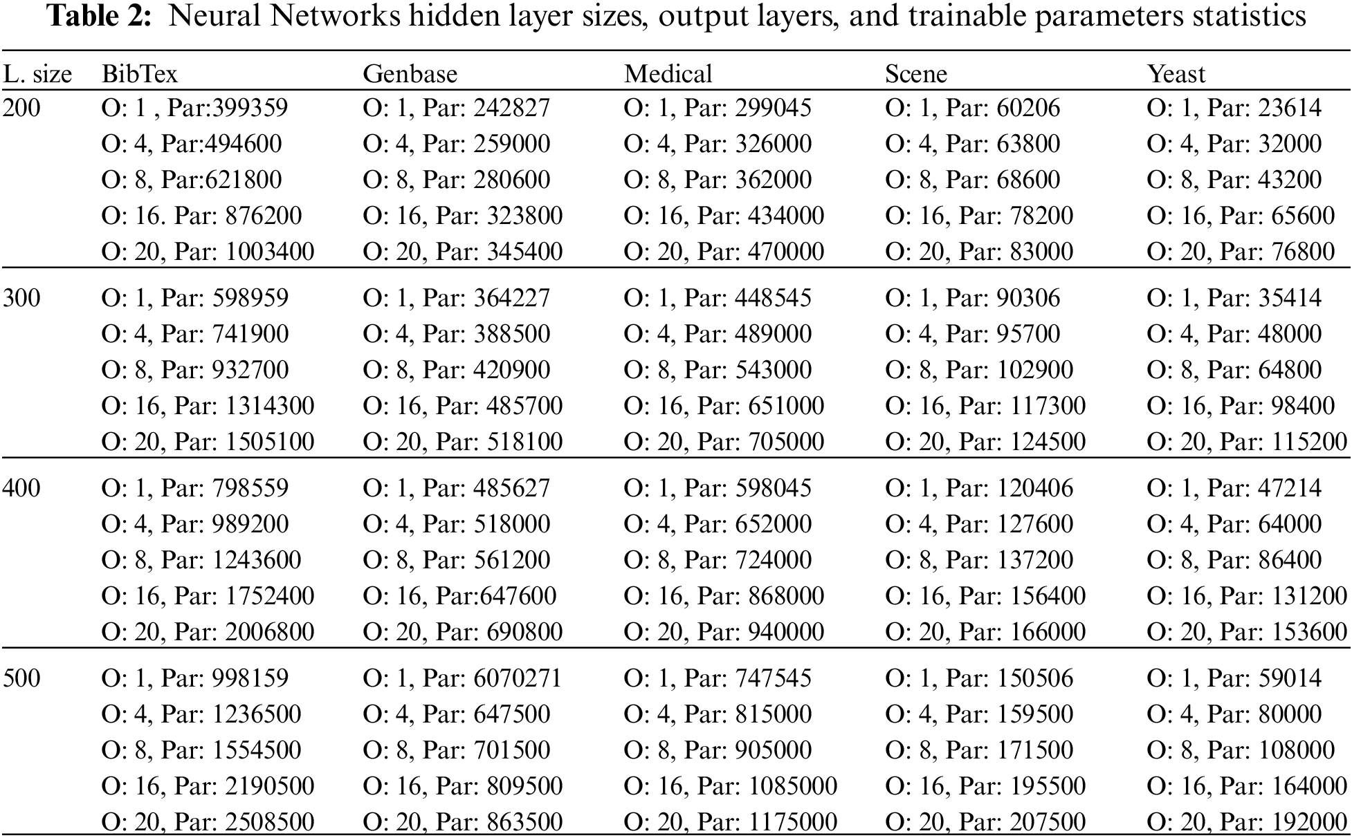
The number of trainable parameters steadily increases whenever we add output layers to the neural network Tab. 2. The trainable parameters for a single output layer and 20 output layers increased by 60%, 30%, 36%, 27%, and 69% for BibTeX, Genbase, Medical, Scene, and Yeast datasets, respectively. The difference in the increment percentage between different datasets is attributed to the number of labels, cardinality, distinct, and other dataset characteristics.
The output of the hidden layer is transformed using a rectified linear activation function (ReLU) to achieve non-linearity in the mapping between inputs and outputs. The hidden layer and the output layers weights are initialized using a Glorot uniform initializer that picks samples from a uniform distribution within a predefined range. Although the samples were drawn randomly, seeds are assigned for the random number generators in the global session, programming language virtual environment, and external libraries to enable experiments reproducibility. Adam is used as an optimization algorithm with the following settings, a learning rate of 0.001, the first exponential decay rate is set 0.9, and the second exponential decay rate to 0.9. Binary Cross-entropy is the loss function for every component in the output layers with binary accuracy as an evaluation metric in training. The number of training epochs is 300, with batch size set to 128. Finally, 10% of the training set is used for validation in the training process.
Unlike single class and multiclass classification, evaluating multi-label classification models is not straightforward. Most of the multi-label datasets are imbalanced, invalidating the reliability of traditional accuracy as an evaluation metric. Several evaluation metrics for multi-label classification measure the performance of the classification models. The following is a list of metrics used in this work with a brief description.
• Weighted F1-Measure: The standard F1-measure is often described as the harmonic mean of precision and recall. Precision can be obtained by dividing the number of true positives (TP) predicted by the model by all the instances marked as positive, which include the false positives (FP).
On the other hand, recall is the number of true positives predicted by the model divided by the number of positive instances that the model should have predicted.
The weighted F1-Measure differs from the standard F1-measure by giving weights to each class in the dataset equal to class probability. The classes with more instances receive higher weights than those with fewer instances.
• Micro-F1 Measure: In micro F1-measure, all the true positives, false positives, and false negatives are computed globally regardless of the classes. Then the micro-precision and micro-recall are calculated based on the micro TP, FP, and FN. Finally, the Micro F1-Measure is obtained by finding the harmonic mean of the micro-precision and recall. The micro F1-Measure is a better evaluation metric for multi-label classification than weighted F1-Measure since it treats all instances equally.
• Macro-F1 Measure: Macro-F1 Measure does not consider data imbalance because it equally treats all the classes in the datasets. The macro TP, FP, and FN are computed for each class. This approach will favor classes with more examples in the dataset since the classifier will most likely be skewed towards them.
• Samples-F1 Measure: This metric is one of the better evaluation metrics among the other variations of the F1 measures. Samples-F1 Measure is computed by averaging the TPs, FPs, and FPs of each instance, which is very helpful in evaluating the performance classifiers on multi-label classification problems.
• Subset Accuracy (Exact Matching Ration): Subset Accuracy is calculated by dividing the number of instances that have been correctly predicted for all the class labels in the labels set over the total number of instances. While Subset accuracy is a good metric for evaluating the classifier’s ability to identify the exact instances’ classes, it disregards the correct labels within the label set of the other instances.
• Hamming Loss: Hamming loss counts for the misclassified labeled within the instance label set. It computes the exclusive-or of the predicted labels set and instance true label set
• Ranking Loss: Ranking loss is the percentage of incorrectly ordered classes to correctly ordered classes. The lower is the ranking loss of a classifier, the better it is. The ground truth of the binary matrix of the ordered labels is defined as
where
We examine the performance of the 20 intelligent models in classifying the labels of 5 multi-label classification datasets. As seen in Figs. 4–8, the models behaved differently on BibTeX, Genbase, Medical, Scene, and Yeast datasets. We selected four evaluation metrics out of the seven metrics included in this work to be plotted in the figures for simplicity and clarity. Weighted-F1 Measure, Subset Accuracy, Hamming Loss, and Ranking Loss are the selected evaluation metrics. At some point, the ENSOCOM models outperformed those with a single output layer for all the datasets. Sometimes models with the same number of output layers and hidden layer size improved on some metrics, but not all.
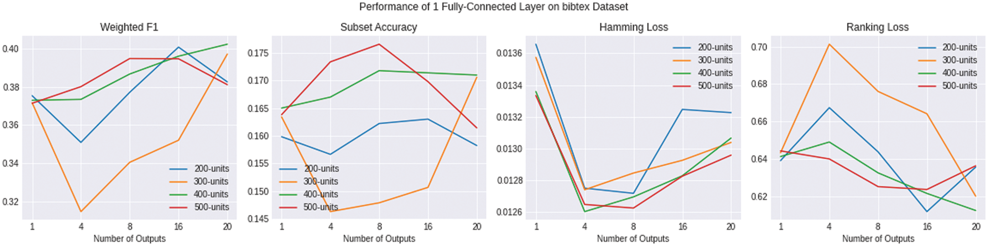
Figure 4: Shows the evaluation of multiple variations of ENSOCOM models in comparison to single-output network models based on W-F1↑, Sub-Acc↑, Ham-Loss↓, Rank-Loss↓ metrics for the BibTeX dataset
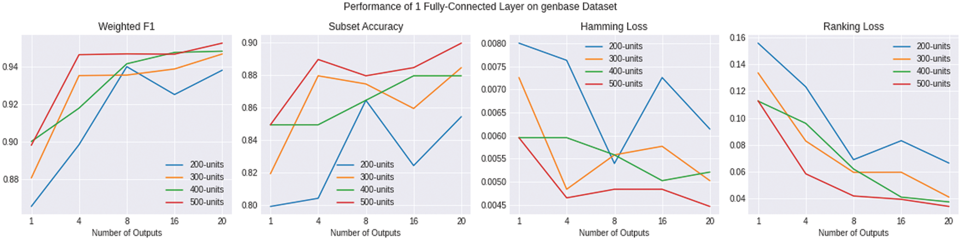
Figure 5: Shows the evaluation of multiple variations of ENSOCOM models on the Genbase dataset
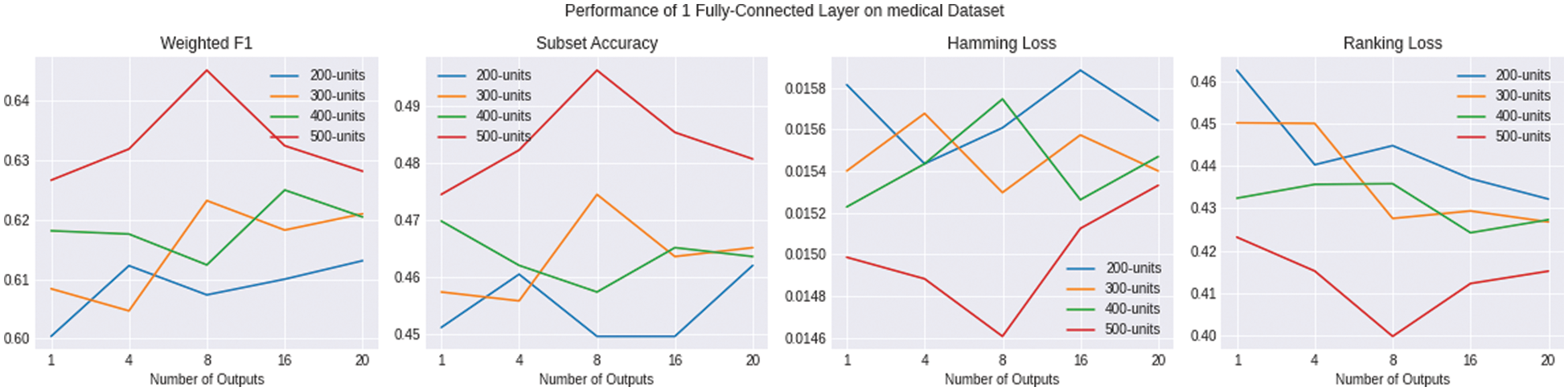
Figure 6: Shows the evaluation of multiple variations of ENSOCOM models on the Medical dataset
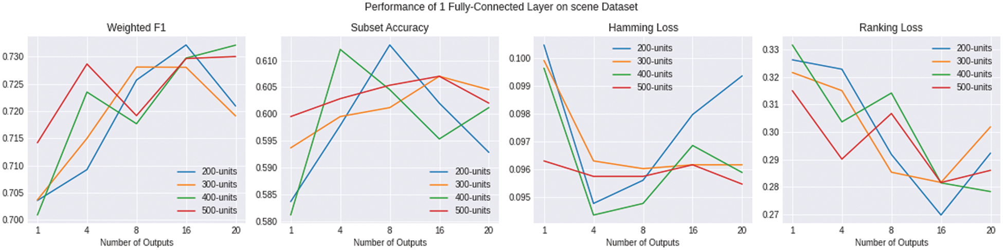
Figure 7: Shows the evaluation of multiple variations of ENSOCOM models on the scene dataset
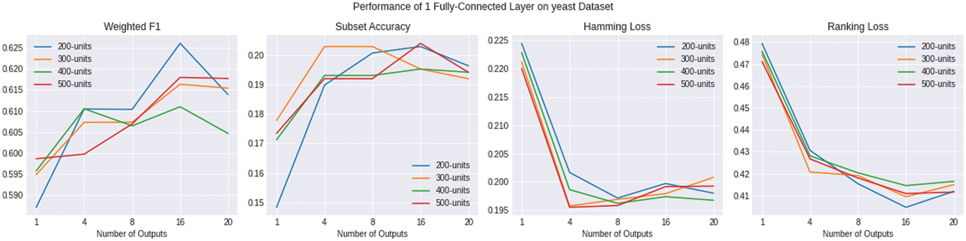
Figure 8: Shows the evaluation of multiple variations of ENSOCOM models on the yeast dataset
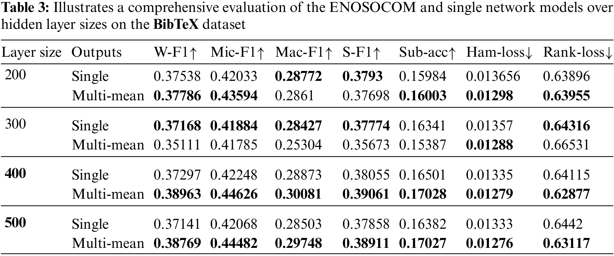
Fig. 4 shows that the multioutput models achieved better scores on the BibTeX dataset depending on the number of output layers. For instance, The best weighted-F1 score for networks with 100 and 500 neurons in the hidden layer was with 16 output layers. The models with 300 and 400 neurons in the hidden layer reported their highest W-F1 score with 20 output layers. Models with fewer neurons in the hidden layer had better Subset Accuracy with more output layers. The improvement of models in terms of their Hamming Loss score is much more evident than the previous two metrics; all the ENSOCOM models reported better Hamming Loss than the single output mode. Similar to Weighted-F1, fewer neurons need more outputs to outperform the single output model to improve the Ranking Loss metric. Tab. 3 shows the mean of all the evaluation metrics achieved by the ENSOCOM models to evaluate the proposed methodology better. By comparing the single output performance to the mean of the results obtained from the ENSOCOM models, we found that ENSOCOM models with 16 output layers outperformed other models on all metrics except for Ranking Loss.
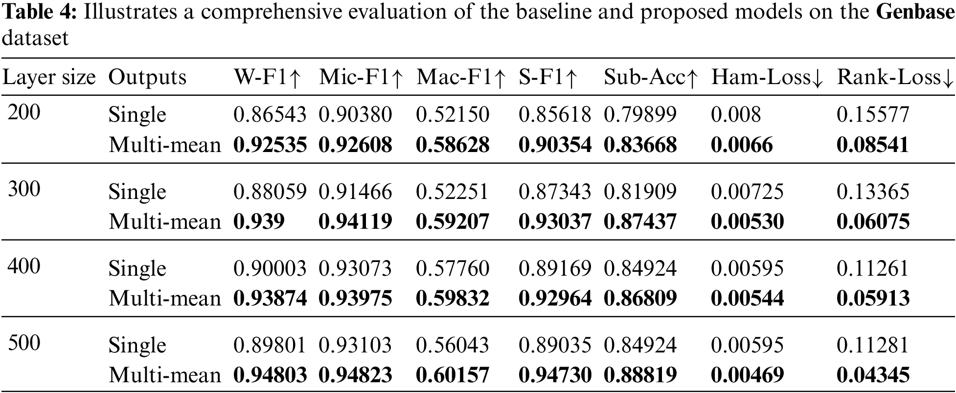
The performance of the ENSOCOM models is better recognized on the Genbase dataset. The single output layer never outperformed the ENSOCOM models on any evaluation metric regardless of the number of output layers, as illustrated in Fig. 5. The difference between the ENSOCOM models and single output models’ performance becomes apparent in Tab. 4. The Table shows that the ENSOCOM model with 500 hidden layer neurons reported the highest scores for all evaluation metrics.
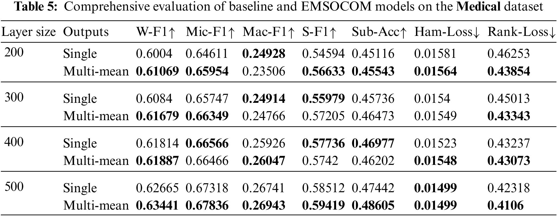
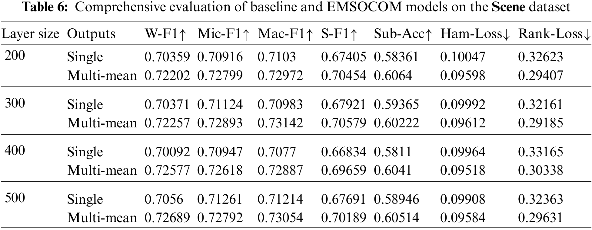
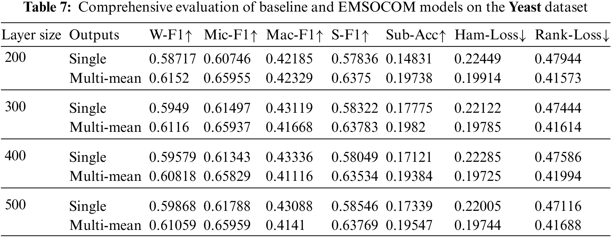
The size of the hidden layer and the number of output layers impact the performance of the ENSOCOM models on the Medical dataset. Models with larger hidden layer sizes are better than the low ones. We can see a tradeoff between the Weighted-F1 Measure and Hamming Loss evaluation metric, where the ENSOCOM models reported better loss and lower F1-score than the single output model Fig. 6. However, the overall performance of ENSOCOM models with 500 neurons in the hidden layers outperformed the baseline models Tab. 5. Moreover, the ENSOCOM model variations outperformed all the Scene dataset baseline models, see Fig. 7. The difference between the baseline models’ performance and the proposed small-sized models is more significant than the larger ones. However, models with more neurons in the hidden layer showed the potential for improvement with more output layers. Unlike the previous datasets, the best overall performance of the ENSOCOM models was not limited to models with a high number of neurons Tab. 6. The same applied to the performance of the ENSOCOM models on the Yeast dataset Fig. 8 and Tab. 7. Hence, the two datasets do not need models with many output layers for most evaluation metrics. We further validated the proposed method’s performance by computing the Paired t-Test to compare the means of the results obtained by single output and ENSOCOM models on all the datasets. The P-value of the paired t-test is 8.882e−15, which means the null hypothesis is rejected, and the improvement of the ENSOCOM over single output models is statistically significant.
The previous experiments proved that ENSOCOM network models are better than traditional ones. On some datasets, the degree of improvement is more significant than the others. To study the reasons behind this, we conduct a correlation analysis between the degree of improvements of all ENSOCOM models with datasets cardinality, density, and distinct. We used two correlation algorithms known as Spearman’s rank correlation and Pearson correlation. Tab. 8 shows correlations coefficients between evaluation metrics and the size of hidden layers in the ENSOCOM. There is no clear pattern for both coefficients over hidden layer size variations. The correlation coefficients for the loss metrics are more consistent over different network models than the Weighted-F1 and Subset Accuracy.
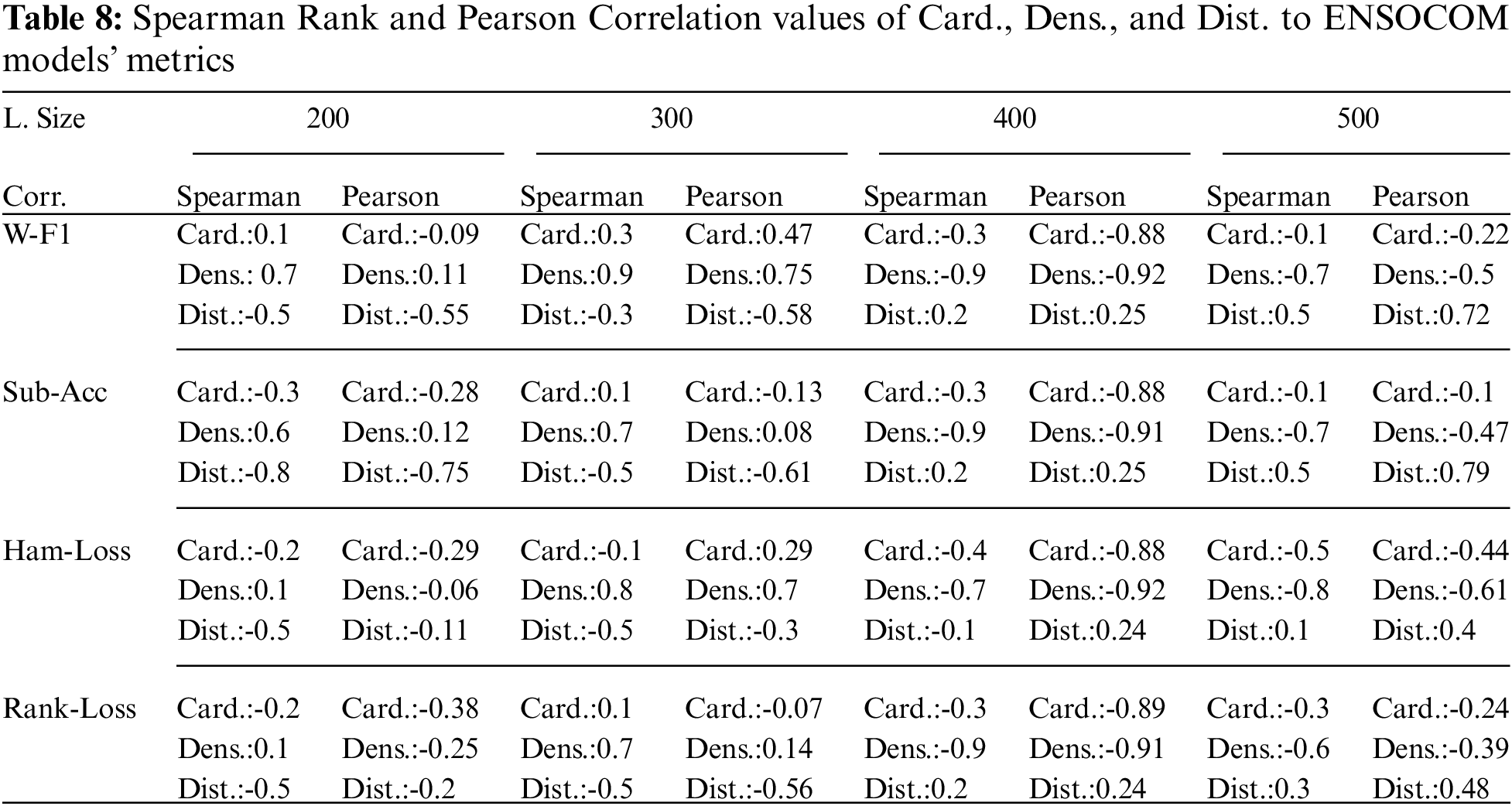
Spearman’s rank and Pearson agree on the negative relationship between dataset distinct and Weight-F1. The higher the number of distinct labels in the dataset, the lower the Weighted-F1. Moreover, Subset Accuracy suffers from the same problem, and it is highly affected by the number of distinct labels in the multi-label datasets. On the other hand, high dataset density result is in better Subset Accuracy, so both move in the same direction. While density has a negative relationship with Hamming Loss and Ranking Loss, it is beneficial since the lower the loss, the better model. Also, Pearson consistently reports a significantly negative relationship between cardinality and Hamming Loss. Spearman’s rank agrees with Pearson on the negativity of the relationship between cardinality and Hamming Loss, but not with high confidence.
ENSOCOM proved that the ensemble of multiple output layer-based classifiers with the same hidden layer reported better results than the conventional single output layer neural networks. By experimenting with various multi-label data domains, the ENSOCOM improved the network’s predictions performance regardless of the data type. We found that the optimal number of output layers and hidden layer sizes are data-dependent and not generalized. The change in the number of parameters from single to multioutput layers is also dependent on the dataset statistical characteristics. There are still many research directions to explore the applications more applications for ENSOCOM. The proposed method can be incorporated into more complex deep neural networks for better evaluation.
Acknowledgement: The authors would like to thank the Deanship of Scientific Research at Umm Al-Qura University for supporting this work by Grant Code: (22UQU4340018DSR02).
Funding Statement: The authors would like to thank the Deanship of Scientific Research at Umm Al-Qura University for supporting this work by Grant Code: (22UQU4340018DSR02).
Conflicts of Interest: The author declares that they have no conflicts of interest to report regarding the present study.
1. S. Rayana, W. Zhong and L. Akoglu, “Sequential ensemble learning for outlier detection: A bias-variance perspective,” in The 16th Int. Conf. on Data Mining (ICDM), Barcelona, Spain, IEEE, pp. 1167–1172, 2016. [Google Scholar]
2. D. Xu, Y. Shi, I. W. Tsang, Y. -S. Ong, C. Gong et al., “Survey on multi-output learning,” IEEE Transactions on Neural Networks and Learning Systems, vol. 31, no. 7, pp. 2409–2429, 2019. [Google Scholar]
3. P. Liu, X. Qiu and X. Huang, “Recurrent neural network for text classification with multitask learning,” arXiv preprint arXiv:1605.05101, 2016. [Google Scholar]
4. M. Sajjad, S. U. Khan, N. Khan, I. U. Haq, A. Ullah et al., “Towards efficient building designing: Heating and cooling load prediction via multi-output model,” Sensors, vol. 20, no. 22, pp. 6419, 2020. [Google Scholar]
5. S. Li, Z. -Q. Liu and A. B. Chan, “Heterogeneous multitask learning for human pose estimation with deep convolutional neural network,” in Proc. of the IEEE Conf. on Computer Vision and Pattern Recognition Workshops (CVPR), Columbus, Ohio, pp. 482–489, 2014. [Google Scholar]
6. X. Sun, J. Xu, C. Jiang, J. Feng, S. -S. Chen et al., “Extreme learning machine for multi-label classification,” Entropy, vol. 18, no. 6, pp. 225, 2016. [Google Scholar]
7. W. Farlessyost, K. -R. Grant, S. R. Davis, D. Feil-Seifer and E. M. Hand, “The effectiveness of multi-label classification and multi-output regression in social trait recognition,” Sensors, vol. 21, no. 12, pp. 4127, 2021. [Google Scholar]
8. M. -L. Zhang, Y. -K. Li, X. -Y. Liu and X. Geng, “Binary relevance for multi-label learning: An overview,” Frontiers of Computer Science, vol. 12, no. 2, pp. 191–202, 2018. [Google Scholar]
9. A. Onan, “Classifier and feature set ensembles for web page classification,” Journal of Information Science, vol. 42, no. 2, pp. 150–165, 2016. [Google Scholar]
10. A. Onan, “An ensemble scheme based on language function analysis and feature engineering for text genre classification,” Journal of Information Science, vol. 44, no. 1, pp. 28–47, 2018. [Google Scholar]
11. W. Sun, G. Dai, X. Zhang, X. He and X. Chen, “TBE-Net: A three-branch embedding network with part-aware ability and feature complementary learning for vehicle re-identification,” IEEE Transactions on Intelligent Transportation Systems, Early Access, pp. 1–13, 2021. [Google Scholar]
12. W. Sun, L. Dai, X. R. Zhang, P. S. Chang and X. Z. He, “RSOD: Real-time small object detection algorithm in UAV-based traffic monitoring,” Applied Intelligence, vol. 51, pp. 1–16, 2021. [Google Scholar]
13. G. Tsoumakas, A. Dimou, E. Spyromitros, V. Mezaris, I. Kompatsiaris et al., “Correlation-based pruning of stacked binary relevance models for multi-label learning,” in Proc. of the 1st Int. Workshop on Learning from Multi-Label Data, Bled, Slovenia, pp. 101–116, 2009. [Google Scholar]
14. J. Read, B. Pfahringer, G. Holmes and E. Frank, “Classifier chains for multi-label classification,” Machine Learning, vol. 85, no. 3, pp. 333–359, 2011. [Google Scholar]
15. L. E. Sucar, C. Bielza, E. F. Morales, P. Hernandez-Leal, J. H. Zaragoza et al., “Multilabel classification with Bayesian network- based chain classifiers,” Pattern Recognition Letters, vol. 41, pp. 14–22, 2014. [Google Scholar]
16. G. Tsoumakas and I. Vlahavas, “Random k-labelsets: An ensemble method for multi-label classification,” in Proc. 18th European Conf. on Machine Learning, Warsaw, Poland, Springer, pp. 406–417, 2007. [Google Scholar]
17. P. Szyma ́nski, T. Kajdanowicz and K. Kersting, “How is a data-driven approach better than random choice in label space division for multi-label classification?” Entropy, vol. 18, no. 8, pp. 282, 2016. [Google Scholar]
18. J. Read, B. Pfahringer and G. Holmes, “Multilabel classification using ensembles of pruned sets,” in Proc. 8th IEEE Int. Conf. on Data Mining, Washington, DC, United States, IEEE, pp. 995–1000, 2008. [Google Scholar]
19. M. L. Zhang and Z. H. Zhou, “Ml-knn: A lazy learning approach to multi-label learning,” Pattern Recognition, vol. 40, no. 7, pp. 2038–2048, 2007. [Google Scholar]
20. C. Vens, J. Struyf, L. Schietgat, SĎ zeroski and H. Blockeel, “Deci-sion trees for hierarchical multi-label classification,” Machine Learning, vol. 73, no. 2, pp. 185, 2008. [Google Scholar]
21. J. Wehrmann, R. Cerri and R. Barros, “Hierarchical multi-label classification networks,” in Proc. 35th Int. Conf. on Machine Learning, Stockholmsmässan, Sweden, PMLR, pp. 5075–5084, 2018. [Google Scholar]
22. A. Elisseeff and J. Weston, “A kernel method for multi-labelled classification,” Advances in Neural Information Processing Systems, vol. 14, pp. 681–687, 2001. [Google Scholar]
23. Y. -Y. Yang, Y. -A. Lin, H. -M. Chu and H. -T. Lin, “Deep learning with a rethinking structure for multi-label classification,” in Proc. the 11th Asian Conf. on Machine Learning, Nagoya, Japan, PMLR, pp. 125–140, 2019. [Google Scholar]
24. A. Maxwell, R. Li, B. Yang, H. Weng, A. Ou et al., “Deep learning architectures for multi-label classification of intelligent health risk prediction,” BMC Bioinformatics, vol. 18, no. 14, pp. 121–131, 2017. [Google Scholar]
25. J. Du, Q. Chen, Y. Peng, Y. Xiang, C. Tao et al., “Ml-net: Multi-label classification of biomedical texts with deep neural networks,” Journal of the American Medical Informatics Association, vol. 26, no. 11, pp. 1279–1285, 2019. [Google Scholar]
26. F. Gargiulo, S. Silvestri, M. Ciampi and G. De Pietro, “Deep neural network for hierarchical extreme multi-label text classification,” Applied Soft Computing, vol. 79, pp. 125–138, 2019. [Google Scholar]
27. S. Wang, A. Raju and J. Huang, “Deep learning based multi-label classification for surgical tool presence detection in laparoscopic videos,” in Proc. 14th Int. Symp. on Biomedical Imaging (ISBI 2017), Melbourne, Australia, IEEE, pp. 620–623, 2017. [Google Scholar]
28. G. Haralabopoulos, I. Anagnostopoulos and D. McAuley, “Ensemble deep learning for multi-label binary classification of user-generated content,” Algorithms, vol. 13, no. 4, pp. 83, 2020. [Google Scholar]
29. M. V. Narkhede, P. P. Bartakke and M. S. Sutaone, “A review on weight initialization strategies for neural networks,” Artificial Intelligence Review, vol. 55, no. 1, pp. 291–322, 2021. [Google Scholar]
30. G. Tsoumakas, I. Katakis and I. Vlahavas, “Mining multi-label data,” in Data Mining and Knowledge Discovery Handbook, New York City, USA: Springer, pp. 667–685, 2009. [Google Scholar]
31. I. Katakis, G. Tsoumakas and I. Vlahavas, “Multi-label text classification for automated tag suggestion,” in Proc. of the European Conf. on Machine Learning and Principles and Practice of Knowledge Discovery in Databases (ECML PKDD), Antwerp, Belgium, Citeseer, vol. 18, pp. 5, 2008. [Google Scholar]
32. S. Diplaris, G. Tsoumakas, P. A. Mitkas and I. Vlahavas, “Protein classification with multiple algorithms,” in Proc. 10th Panhellenic Conf. on Informatics, Volos, Greece, Springer, pp. 448–456, 2005. [Google Scholar]
33. J. Pestian, C. Brew, P. Matykiewicz, D. J. Hovermale, N. Johnson et al., “A shared task involving multi-label classification of clinical free text,” in Proc. Biological, Translational, and Clinical Language Processing, Prague, Czech Republic, pp. 97–104, 2007. [Google Scholar]
34. M. R. Boutell, J. Luo, X. Shen and C. M. Brown, “Learning multi-label scene classification,” Pattern Recognition, vol. 37, no. 9, pp. 1757–1771, 2004. [Google Scholar]
 | This work is licensed under a Creative Commons Attribution 4.0 International License, which permits unrestricted use, distribution, and reproduction in any medium, provided the original work is properly cited. |