Computers, Materials & Continua DOI:10.32604/cmc.2022.021781
Article

Construction of an Energy-Efficient Detour Non-Split Dominating Set in WSN

G. Sheeba1,* and T. M. Selvarajan2

1Department of Mathematics, Government Engineering College, Trivandrum, 695035, India
2Department of Mathematics, Noorul Islam Centre for Higher Education, Kumaracoil, Thuckalay, 629175, India
*Corresponding Author: G. Sheeba. Email: gsheeba1234@gmail.com
Received: 14 July 2021; Accepted: 16 November 2021

Abstract: Wireless sensor networks (WSNs) are one of the most important improvements due to their remarkable capacities and their continuous growth in various applications. However, the lifetime of WSNs is very confined because of the delimited energy limit of their sensor nodes. This is the reason why energy conservation is considered the main exploration worry for WSNs. For this energy-efficient routing is required to save energy and to subsequently drag out the lifetime of WSNs. In this report we use the Ant Colony Optimization (ACO) method and are evaluated using the Genetic Algorithm (GA), based on the Detour non-split dominant set (GA) In this research, we use the energy efficiency returnee non-split dominating set (DNSDS). A set S ⊆ V is supposed to be a DNSDS of G when the graph G = (V, E) is expressed as both detours as well as a non-split dominating set of G. Let the detour non-split domination number be addressed as γ_dns (G) and is the minimum order of its detour non-split dominating set. Any DNSDS of order γdns(G) is a γdns-set of G. Here, the γ_dns (G) of various standard graphs is resolved and some of its general properties are contemplated. A connected graph usually has an order n with detour non-split domination number as n or n – 1 are characterized. Also connected graphs of order n≥4 and detour diameter D≤4 with detour non-split dominating number n or n−1 or n−2 are additionally portrayed. While considering any pair of positive integers to be specific a and b, there exists a connected graph G which is normally indicated as dn(G)=a, γ(G)=b and γdns(G) = a + b − 2, here γdns(G) indicates the detour domination number and dn(G) indicates the detour number of a graph. The time is taken for the construction and the size of DNSDS are considered for examining the performance of the proposed method. The simulation result confirms that the DNSDS nodes are energy efficient.

Keywords: Domination number; non-split domination number; detour number; detour non-split domination number

1  Introduction

In WSN, for its capability of detection and processing the substantial section of the sensor node is often set in massive sums. These sensor nodes collect information from the viewing zone and the base station. Communication is the primary role of the WSN. Each sensor node is energy-protected here [1]. The delay and the duration of transmission are to be reduced each time when the packet is exchanged. To do so, the nodes have to be energy-rich [2]. In WSN, communication is carried out with the backbones, only the set of nodes. It may be able to generate backbones through the use of DNSDS [3]. Treat the packet from one bundle to the next until DNSDS nodes reach the destination. The backbone usage reduces overhead communication [4], builds capacity for data transmission, and reduces packet latency.

In this article, we design a population-based search technique specifically for the ACO which is supported by ant behavior in the creation of EE-DNSDS to provide answers to the optimization problem [5]. It evaluates its performance against the DNSDS based on the GA. The GA approach is a search solution both for the population and for natural biological development [6]. The rest of the paper is as follows: The notion of developing a DNSDS is outlined in Section 2. The background of the work is presented in Section 3. The suggested work is presented in Section 4. Section 5 explains experimental evaluation together with settings of stimulation, performance measures, and evaluation results. Section 6 provides for the conclusion.

2  Related Work

We consider graph G as finite, undirected, and connected lacking loops. Let the order of G be denoted as p and its size be denoted as q respectively. For knowing more about the basic terminologies in graph theory, consider two edges, that are said to be adjacent when both the vertices (i.e.,) are in edge G. Incase when uv∈E(G), then we can easily say that the edge u is a neighbor of v and it is represented using the notation N(v) that is nothing but the neighbor set of edge v. The vertex degree v∈V is deg(v)=|N(v)|. A vertex v is understood as a universal vertex when deg(v)=p−1. The subgraph stimulated by set S of vertices of G is symbolized as <Si> with V(<Si>) = S and E(<Si>) = {uv∈E(G):u,v∈S}. The path that exists between two vertices of a graph and the one which visits each vertex just one time is said to be the Hamiltonian path or Hamilton path. Incase if there is a Hamiltonian path with adjacent endpoints, the resultant graph cycle is described as a Hamiltonian cycle.

In a connected graph G with two vertices namely u and v; the distance denoted as d(u,v) among two vertices is the length of a shortest u−v path in G. Usually, the u−v geodesic is indicated as the u−v path which has the length d(u,v). Let x be a vertex that is understood to lie on a u−v geodesic P, x is a vertex of P together with the vertices namely u and v. The closed interval I[u,v] encloses the vertices u and v along with every vertex within the u−v geodesic. Incase when I[u,v]={u,v} then u and v are said to be adjacent. For a set S of vertices, let I[S]=∪u,v∈SI[u,v]. Then certainly S⊆I[S]. A set S⊆V(G) is supposed to be a geodetic set of G when I[S]=V. The geodetic number is usually denoted as g(G) and a graph is expressed as the minimum order of its geodetic sets and any geodetic set of order g(G) is a g-set of G. The g(G) of graphs was studied in [7–14].

In any connected graph G, with two vertices u and v, the detour distance D(u,v) is defined as the length of the longest u−v path in G. The u−v detour is indicated as the u−v path of length D(u,v). ). Let x be a vertex that is understood to lie on a u−v detour P, x is a vertex of P together with the vertices namely u and v. The utmost detour distance from v to a vertex of G is the detour eccentricity eD(v) of a vertex v in G. The least eD(v) amid the vertices of G is the detour radius, radD(G) of G and the utmost eD(v) is the detour diameter, diamD(G) of G. We denote detour radius by R and detour diameter by D. The closed interval ID[u,v] for two vertices u and v, includes all the vertices that exist within a u−v detour along with u and v. For a set S of vertices, let ID[S]=∪u,v∈DID[u,v]. Then certainly, S⊆ID[S]. A set S⊆V is termed as detour set if ID[S] = V. The detour number dn(G) of G is usually in the least order of its detour sets as well as any detour set of order dn(G) is called a dn− set of G and is initiated and studied in [15–19]. A set S⊆V is termed as dominating set of G if for each v∈V∖S is adjacent to some vertex in S. A dominating set S is said to be minimal if no subset of S is dominating set G. The domination number of G is symbolized as γ(G) and is the minimum cardinality of a minimal dominating set of G and was studied in [20]. Dominating Sets and Domination Polynomial of Fan Related Graphs were studied in [21]. A dominating set D is supposed to be a non-split dominating set of G if <V−D> is connected. The minimum cardinality of a non-split dominating set of G is called the non-split domination number of G and is denoted by γns(G) is called γns-set of G and is deliberated in [22].

3  Background

Ant Colony Optimization (ACO) is appropriate to track optimum paths depending on the behavior of the ants used to look through the food. When a food source is found, it goes back to the province by leaving ‘marks’ (predominantly called pheromones) which signals how much food is available. If others approach the marks, they have a certain probability and they will follow the path. In this event, it is not an easy for others to replenish the food with their own markings. The pathway is located by other ants and is further grounded till some ants flood the province from diverse food sources. As they release pheromones when transporting the food, a shorter path is bound to be more grounded, improving the “solution.” Meanwhile, few ants continue to search for food sources closer to home. When the food resource is depleted, the path is no longer established with pheromones and eventually decays. Because the ant-colony moves in a fairly dynamic manner, and the ACO performs better in graphs with changing topologies. Examples of such frameworks include computer networks and worker artificial intelligence simulations.

3.1 The Detour Non-Split Domination Number of a Graph

A set S ⊆ V is a Detour Non-Split Dominating Set (DNSDS) of G when the graph G = (V, E) is expressed as both detours as well as a non-split dominating set of G. Let the detour non-split domination number be addressed as γ_dns (G) and is the least order of its DNSDS. Any DNSDS of order γdns(G) is a γdns-set of G.

Example 3.2.2: Assume a graph G in Fig. 1, with no two-element subset of G is a DNSDS of G and so γdns(G) ≥ 3. Let S={v1,v4,v9}. Then S is a DNSDS of G consequently γdns(G) = 3.

Observation:

(i)       All end vertex of a connected graph, G belongs to every DNSDS of G.

(ii)      Let order of G be n≥3 with v as its cut vertex, then every DNSDS of G carries a minimum of a single element from each component of G−v.

(iii)     For the star G=K1,n−1(n≥3),γdns(G)=n.

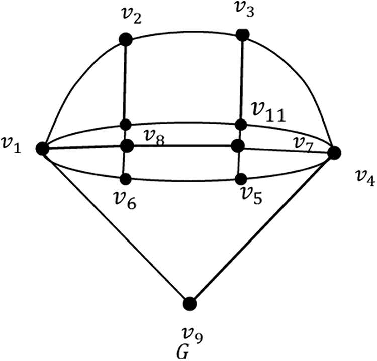
Figure 1: Graph G is a DNSDS of G

• Theorem 1: For the path G=Pn(n≥4), γdns(G) = n−2.

• Proof: Let Pn be v1,v2,…,vn. Then S=V−{v2,v3} is a DNSDS of G accordingly γdns(G) ≤ n−2. We prove that γdns(G) = n−2. In contrast, suppose γdns(G) ≤ n−3. In that case, S′ of G is available then | S′| ≤ n−3. Now <V − S′> is a path P such that |P|≥3. Let vi′ be an internal vertex of P. Then vi′ is not dominated by any vertex of S′. Hence S′ is not a DNSDS of G, there is a negation. As a result γdns(G)=n−2.

• Theorem 2: For the cycle G=Cn(n≥4),γdns(G) = −2.

• Proof: This is alike the attestation of Theorem 3.2.4.

• Theorem 3: For the complete bipartite graph G=Km,n(2≤m≤n), γdns(G) = 2.

• Proof: Assume L and W as bipartite sets of G and xy∈E(G). Then S={x,y} is a DNSDS of G thus γdns(G) = 2.

• Theorem 4: For wheel G=Wn=K1+Cn−1(n≥4),γdns(G) = 2.Proof: Let V(K1)=x and y∈V(Cn−1). Then S={x,y} is a DNSDS of G with the intention that γdns(G) = 2.

• Theorem 5: For the complete graph G=Kn(n≥3),γdns(G) = 2.

• Proof: Let xy∈E(G). Then S={x,y} is a DNSDS of G thus γdns(G) = 2.

• Theorem 6: For double star G of order (n≥4),γdns(G) = 2.

• Proof: Let the set, S carries n−2 end vertices of G. By Observation 3.2.3 (i), S is a subset of each DNSDS of G and as a result γdns(G) ≥ n−2. Since S is a DNSDS of G, it goes with γdns(G) = n−2.

• Theorem 7: For helm graph G=Hr, γdns(G)= r+1.

• Proof: Assume x as central vertex and Z as the set of r end vertices of G. By Observation 3.2.3 (i), Z is a subset of each DNSDS of G. Since x is not subjugated by any vertex of Z,Z is not a DNSDS of G thus γdns(G) ≥ r+1. Let Z′ = Z∪{x}. Then ID[Z′] = V and <V−Z′> doesn’t have isolated vertices. As a result Z′ is a DNSDS of G and γdns(G) = r+1.

• Theorem 8: For banana tree graph G=Br.s, γdns(G) = r+1.

• Proof: Assume x as central vertex and Z as the set of r end vertices of G. By Observation 3.2.3 (i), Z is a subset of each DNSDS of G. Since x is not subjugated by any vertex of Z, Z is not a DNSDS of G thus γdns(G) ≥ r+1. Let Z′=Z∪{x}. Then ID[Z′] = V and <V − Z′> doesn’t have isolated vertices. As a result Z′ is a DNSDS of G and γdns(G) = r+1.

• Theorem 9: Assume Regard G as a connected graph with order n≥3 with D≥2. Then γdns(G) ≤ n−1.

• Proof: Assume P:v0,v1,v2,…,vD as a detour diametral path in G. As D≥2,P contains at least one internal vertex. Let S=V−{v1}. The S is a DNSDS of G with γdns(G) ≤ n−1.

• Remark 10: The bound in Theorem 3.2.12 is spiky. For path G=P3, γdns(G) = 2 =n−1.

• Theorem 11: Assume Regard G as a connected graph with order n≥2. Also γdns(G) = n as long as G is K2.

• Proof: Let γdns(G) = n. In contrast when G≠K2. By Theorem 3.2.12, γdns(G) ≤ n−1, which is a contradiction. As a result, D=1. Hence G=K2. The reverse is apparent.

• Theorem 12: Regard G as a connected graph with order n≥4 which is not a star. Then γdns(G) ≤ n−2.

• Proof: Assume G as a tree. Since G≠K1,n−1, G holds two adjacent vertices, say x and y. Then S=V(G)−{x,y} is a DNSDS of G so that γdns(G) ≤ n − 2. After that imagine that G is not a tree. Then G includes a cycle says C. Let C:v1,v2,…,vr(r≥3) be the longest cycle in G. Suppose that all the vertices of C are cut-vertices of G. Then S=V(G)−V(C) is a DNSDS of G and so γdns(G) ≤ n−|V(G)|≤n−3, therefore is a negation. Suppose that G holds as a minimum one cut-vertex, say v1. Then S=V(G)−{v1,v2} is a DNSDS of G as a result γdns(G) ≤ n−2, which is a contradiction. If no vertex of G is a cut vertex of G, by the similar argument, it can show that γdns(G) ≤ n−2, which is a contradiction.

• Remark 13: The bound in Theorem 2.15 is spiky. For cycle G=C4, γdns(G) = 2 =n−2.

• Theorem 14: Assume Regard G as a connected graph with order n≥3. Also γdns(G) = n−1 as long as G=K1,n−1 or K3.

• Proof: Let γdns(G) = n−1. If n=3, then G=K1.2 or K3, which satisfies the requirements of this theorem. So we have done. Let n≥4. But when G≠K1,n−1, then according to the Theorem 3.2.15, γdns(G) ≤ n−2, therefore is a negation. For that reason G=K1,n−1. The converse is clear. Now we distinguish connected graph with order n≥4 and detour diameter D≤4 with γdns(G) = n−2. For this purpose, we introduce family I of graph

• Theorem 15: Assume G as a connected graph with n≥4 and D≤4. Then γdns(G) = n−2 as long as G is either C4 or K4 or K4 − {e} or a double star of the graph G specified in Fig. 2 of the family I.

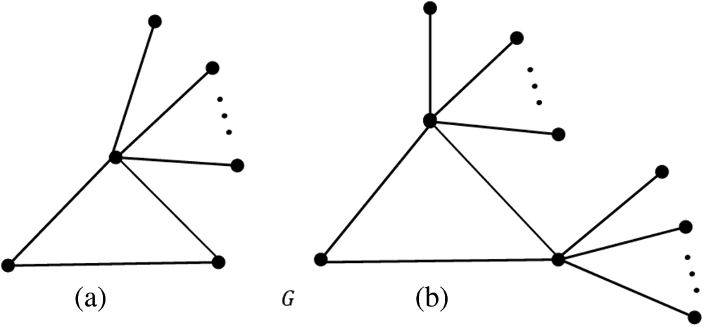
Figure 2: GraphG specified in the family I

• Proof: Let γdns(G) = n−2. So we enclose the two subsequent cases.

• Case (i): If G is a tree. According to Theorem 3.2.17, G≠K1,n−1. Suppose G is a double star, then G satisfies the requirements of this theorem. So, we have done. Let us assume that G is neither a star nor a double star. Then G contains a path P:x,y,z. Let S=V−{x,y,z}. Then S is a DNSDS of a graph as a consequence γdns(G) ≤ n−3, therefore is a negation.

• Case (ii): If G is not a tree. Then it holds as a minimum of one cycle C. Let C be a girth in G and C(G) be its length. Since D≤4. We have that C(G)≤4. Let C be v1,v2,v3,v4,v1. If G=K4−{e}, then we are done. If G=K4, then we are done. Suppose that G is neither C4 nor K4− {e} nor K4. Then there exists one vertex x to such a degree which is adjacent to v1, say. Then S=V−{v1,v2,v3} is a detour non-split domination number of a graph as a result, γdns(G) ≤ n−3, therefore is a negation. Let C(G)=3. Let C be v1,v2,v3,v1. Since D≤4, there exists a minimum of one vertex( x) thereby xv1∈E(G). If d(v2)=d(v3)=2 and the edges incident with v1 are end edges, then the graph G is given in family I of Fig. 2a. This satisfies the requirements of this theorem. If at least one edge incident with x is not an end edge, subsequently γdns(G) ≤ n−3, which is a contradiction. If deg(v1)=2,deg(v2)≥3 and deg(v3)≥3, then since D≤4, the edges incident at v2 and v3 are end edges. Then graph G is given in the family I of Fig. 2b. Since D≤4, deg( vi) ≥ 3 for all i (1 ≤ i ≤ 3) is not possible. The reverse is apparent.

• Theorem 16: While considering whichever pair of positive integers to be specific a and b, there exists a connected graph G thereby dn(G)=a, γ(G)=b and γdns(G) = a+b−2. Proof: Let P2(b−2)+1:x,v1,v2,…,v2(b−2)+2,y be a path on 2(b − 2) + 2 vertices. H as a graph attained from P2(b−2)+2 by accumulating the new vertices x1,x2,…,xa−1 and introduced as edge xxi(1≤i≤a−1). Assume graph G gained from H by summing up new vertices u1,u2,…,ub−2 with initiating the edges uivi(1≤i≤2(b−2)−1) and uivi+1(2≤i≤2(b−2) is revealed in Fig. 3. Since ID[X]=V, X is a detour set of G therefore, dn(G)=a. Subsequently, we illustrate that γ(G)=b. We view that all γ-set of G contains ui(1≤i≤b−2) and the vertices x and y and γ(G)=b−2+2=b. Let S={x,y,u1,u2,…,ub−2}. Then S is a dominating set of G so that γ(G)=b. After that, we show that γdns(G)=a+b−2. The end vertices of G be X={x,x1,x2,…,xa−1,y}. By Observing 3.2.3 (i), X is a subset of every DNSDS of G and so γdns(G) ≥ a. It is handily seen that each DNSDS of G holds each ui(1≤i≤b−2) and so γdns(G) ≥ a+b−2. Let S′ = X ∪ {u1,u2,…,ub−2}. Then S′ is DNSDS of G so that γdns(G) = a+b−2.

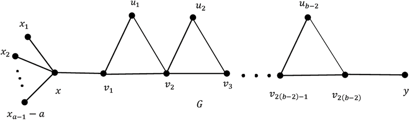
Figure 3: Graph G gained from H by summing up new vertices

3.2 The Detour Non-Split Domination Number of Join of Graph

Assume H and as we K as two graphs. The combination of two graphs namely G and H is symbolized as G+H and defined as the graph with V(G+H)=V(G)∪V(H) and E(G+H)=E(G)∪E(H)∪{uv:u∈V(G),v∈V(H)}.

• Theorem 1: If K and H are two connected graphs that contain either a Hamiltonian path or a Hamiltonian cycle. Then γdns(K+H)=2.

• Proof: Let P1:u0,u1,u2,…,ul be a Hamiltonian path in K, similarly P2:v0,v1,v2,…,vk be a Hamiltonian path in G, where l+k=n. Then P1∪P2 is a Hamiltonian path in K+H. Let S={u0,v0}. Then S is a DNSDS of K+H consequently γdns(K + H) = 2.

• Corollary 2:

(i)    Let K=Pn(n≥4) and H=Pm(m≥4). Then γdns(K+H) = 2.

(ii)    Let K=Pn(n≥4) and H=Cm(m≥4). Then γdns( K+H) = 2.

(iii)    Let K=Cn(n≥4) and H=Cm(m≥4). Then γdns( K+H) = 2.

(iv)    Let K=Kn(n≥3) and H=Km(m≥4). Then γdns( K+H)=2.

(v)    Let K=Kn(n≥4) and H=Pm(m≥4). Then γdns( K+H) = 2.

(vi)    Let K=Kn(n≥4) and H=Cm(m≥4). Then γdns(K + H) = 2.

3.3 The Detour Non-Split Domination Number of Corona Product of Graph

The corona product K∘H is described as the graph gained from K and H by attaining one copy of K and |V(K)| copies of H and then by joining an edge of, all the vertices from the ith-copy of H to the ith-vertex of K, where i=1,2,…,|V(H)|.

• Theorem 1: Assume two connected graphs notably, K as well as H with orders n1 and n2 respectively. If H contains either a Hamiltonian path or a Hamiltonian cycle, then γdns( K∘H)=n1.

• Proof: If n2 = 1, then the result is obvious. Let H1 = ( V1,E1), H2=(V2,E2),…,Hn1=(Vn1,En1) be the n1 copies of H in K∘H. Let Qi:vi1,vi2,…,vin2,(1≤i≤n1) be a Hamiltonian path in Hi(1≤i≤n1). Assume V as the vertex of K and V={v1,v2,…,vn1}. Then set of cut vertices in K∘H is V. By Observing 3.2.3 (ii), every DNSDS of K∘H holds minimum vertex from every Qi(1≤i≤n1) consequently γdns(G) ≥ n1. Let S = { v11,v21,…,vn11}. Then S is a DNSDS of K∘H so that γdns( G) = n1.

• Corollary 2:

(i)    Let K=Pn(n≥4) and H=Pm(m≥4). Then γdns(K∘H) = n.

(ii)    Let K=Pn(n≥4) and H=Cm(m≥4). Then γdns( K∘H)=n.

(iii)    Let K=Cn(n≥4) and H=Cm(m≥4). Then γdns( K∘H) = n.

(iv)    Let K=Kn(n≥3) and H=Km(m≥4). Then γdns( K∘H) = n.

(v)    Let K=Kn(n≥4) and H=Pm(m≥4). Then γdns( K∘H) = n.

(vi)    Let K=Kn(n≥4) and H=Cm(m≥4). Then γdns( K∘H) = n.

• Theorem 3: Assume K as a connected graph with order n1≥2. Then γdns( K∘Kn2) = n1n2.

• Proof: Let V ( K¯n2) = { v1,v2,…,vn2} ( 1≤i≤n1) and Si={vi1,vi2,…,vin2} be the ith copy of K¯n2. Then S = ∪i=1n1 Si is the end vertices set of K∘K¯n2. By Observing 3.2.3 (i), S is a subset of every DNSDS of K∘K¯n2 and so γdns( K∘K¯n2) ≥ n1n2. As S is a DNSDS of G, we have γdns( K∘K¯n2) = n1n2.

• Theorem 4: Assume K as a connected graph with order n2 ≥ 2. Then γdns( K∘P¯n2) = n1.

• Proof: Let V(P¯n2)={v1,v2,…,vn2} and Hi = { vi1,vi2,…,vin2} be the ith copy of P¯n2(1≤i≤n1). By Observation 3.2.3 (ii), every DNSDS of G holds a minimum of one vertex from each Hi and so γdns(( K∘P¯n2) ≥ n1. Then S = { v11,v21,…,vn11} is a DNSDS of G so that γdns( K∘P¯n2) = n1.

• Theorem 5: Assume K as a connected graph with order n2≥2. Then γdns(K∘C¯n2)=2n1, Where n2≥5.

• Proof: Let V( K∘C¯n2) = { v1,v2,…,vn2} and Hi = { vi1,vi2,…,vin2 be the ith copy of C¯n2, ( 1≤i≤n2). In that case, it can be said that every DNSDS of G holds a minimum of two vertices from each Hi(1≤i≤n1) and so γdns(G) ≥ 2 n1. Let S = { v11,v13,v21,v23,…,vn11,vn1n2}. Then S is a DNSDS of G so that γdns(G) = 2 n1.

• Theorem 6: Assume K as a connected graph with order n2 ≥ 2. Then γdns( K∘K¯n2) = 2 n1, where 2≤r≤s.

• Proof: Let U={u1,u2,…,ur} and W={w1,w2,…,ws} as the bipartite sets of Kr,s. Let Hi=Ui∪Wi={ui1,ui2,…,uir}∪{wi1,wi2,…,wis} (1 ≤ i ≤ n1) be the ith copy of Kr,s. Since <U¯i> and <W¯i> are complete graphs for all i (1 ≤ i ≤ n1), every DNSDS of G holds a minimum of two vertices of every Hi (1 ≤ i ≤ n1). For this reason γdns(G) ≥ 2 n1. Let S={u11,u21,…,un1r,w11,w21,…,wn1s}. In that case, we conclude S as DNSDS of G with γdns(G) = 2 n1.

4  Proposed System Model

The scavenging behavior of ants excites ACO. When ants walk, they leave a pheromone trail in each node they pass through. The pheromone likelihood, which is provided on every node, aids in determining the shortest path of food from source to destination. A DNSDS, which is rich in energy, is produced in our suggested study. We use two rules in the ACO algorithm to do this: (i) the pheromone updating rule (which signals the updated for each node and is handled in Eq. (4)) and (ii) the state transition rule (which assists with choosing the next node based on the probability value and is addressed in Eq. (1) [22].

Pik=τiα∑i∈Akτiαniβ(1)

In our algorithm, we start with τ0 in each node of the graph. Ants wander throughout the graph randomly by dropping pheromones on all nodes. In this fashion, the ant iterates N times. During this each chosen node with a high P and E based on the probabilistic state transition criteria is added to the DNSDS.

Pik=τiαniβEiγ∑i∈AkτiαniβEiγ(2)

Ei=REEinitial(3)

The τ of the nodes which are in the DNSDS is refreshed by the pheromone updating rule.

τi=(1−ρ).τi+ρ.τo(4)

In Eq. (4), the value of ρ is always 0 ≤ ρ ≤ 1. The τ of the nodes that are unavailable in the DNSDS is evaporated by Eq. (5).

τi=τi×ρ(5)

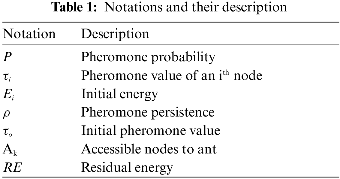
Notations utilized in the work are specified in Tab. 1.

5  Experimental Evaluation

In this section, we have illustrated and investigated fewer limitations, namely the experimental parameters and performance indicators, before presenting the assessment results.

5.1 Simulation Setup

The simulation is completed by assuming the sensor field to be 1000 × 1000. During its execution, the following suspicions are taken into account:

•   Sensor nodes are homogeneous and fixed.

•   The region is both constrained and consistent.

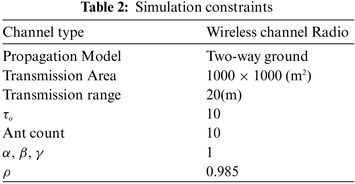
The energy and degree of the node are taken into account during the DNSDS creation process. Using ACO and the GA, we led large-scale replications to create the DNSDS. We have evaluated the effectiveness of both strategies. Tab. 2 specifies the simulated limitations used to raise the EE-DNSDS using the ACO approach.

5.2 Performance Evaluation

The evaluation of the performance is completed by considering two measurements. To be specific the construction time and the size of the DNSDS between the ACO technique and the GA are as follows:

DNSDS Construction Time: Fig. 4 addresses the DNSDS construction time exploited by GA and the ACO technique. While contrasting the ACO and GA, the ACO utilized not as much DNSDS construction time as GA. When the node gets tally to build, the ACO technique performs better when compared to GA.

Figure 4: Comparison of DNSDS construction time

DNSDS Size: Fig. 5 addresses the simulation yield of DNSDS size for different quantities of nodes. We have considered the DNSDS is off to be in average size. In the projected system, the DNSDS size is low in ACO than the GA for the more modest number of nodes. As the node count gets expanded, the average DNSDS size of ACO is lower than the GA.

Figure 5: Comparison of DNSDS size

6  Conclusion

By modifying the ACO approach, we created an Energy Efficient Detour Non-Split Dominating Set (EE-DNSDS) in this paper. The scavenging behavior of ants inspires the ACO process. The DNSDS created an abundance of energy. The correlation between two algorithms, specifically the ACO and the GA, is performed here. When comparing the ACO and GA, the ACO used less DNSDS build time than the GA. As the number of nodes increases, the average DNSDS size of ACO is roughly equal to that of GA. This is accomplished by employing the network’s energy-efficient DNSDS nodes. Furthermore, the number of standard graphs is resolved and a fraction of its overall qualities are considered in the detour non-split domination. Other optimization approaches can be used in the future, and performance measures can be checked and compared.

Acknowledgement: The authors would like to thank Noorul Islam Centre for Higher Education, also we like to thank anonymous reviewers for their so-called insights.

Funding Statement: The authors received no specific funding for this study.

Conflicts of Interest: The authors declare that they have no conflicts of interest to report regarding the present study.

References

 1.  D. Anusha, J. John and S. J. Robin, “The geodetic hop domination number of complementary prisms,” Discrete Mathematics, Algorithms and Applications, vol. 1, no. 6, pp. 1–10, 2021. [Google Scholar]

 2.  X. Qiu and X. Guo, “On graphs with same distance distribution,” Applied Mathematics, vol. 8, no. 6, pp. 799–807, 2017. [Google Scholar]

 3.  G. Chartrand, F. Harary and P. Zhang, “On the geodetic number of a graph,” Networks, vol. 39, no. 1, pp. 1–6, 2002. [Google Scholar]

 4.  G. Chartrand, G. L. Johns and P. Zhang, “On the detour number and a geodetic number of a graph,” Arscombinatoria, vol. 72, pp. 3–15, 2004. [Google Scholar]

 5.  G. Chartrand, G. L. Johns and P. Zhang, “The detour number of a graph,” Utilitas Mathematica, vol. 64, pp. 97–113, 2008. [Google Scholar]

 6.  J. John and N. Arianayagam, “The total detour number of a graph,” Journal of Discrete Mathematical Sciences and Cryptography, vol. 17, no. 4, pp. 337–350, 2014. [Google Scholar]

 7.  J. John and N. Arianayagam, “The detour domination number of a graph,” Discrete Mathematics, Algorithms and Applications, vol. 9, no. 1, pp. 1750–1756, 2017. [Google Scholar]

 8.  J. John and V. R. S. Kumar, “The total detour domination number of a graph,” Infokara Research, vol. 8, no. 8, pp. 434–440, 2019. [Google Scholar]

 9.  J. John and V. R. S. Kumar, “The open detour number of a graph,” Discrete Mathematics, Algorithms and Applications, vol. 13, no. 1, pp. 2050–2088, 2021. [Google Scholar]

10. J. John, P. A. P. Sudhahar and D. Stalin, “On the (M, D) number of a graph,” Proyecciones Journal of Mathematics, vol. 38, no. 2, pp. 255–266, 2019. [Google Scholar]

11. J. John and D. Stalin, “Distinct edge geodetic decomposition in graphs,” Communications in Combinatorics and Optimization, vol. 6, no. 2, pp. 185–196, 2021. [Google Scholar]

12. J. John and D. Stalin, “Edge geodetic self-decomposition in graphs,” Discrete Mathematics, Algorithms, and Applications, vol. 12, no. 5, pp. 2050–2064, 2020. [Google Scholar]

13. J. John and D. Stalin, “The edge geodetic self decomposition number of a graph,” RAIRO Operations Research, vol. 11, no. 2, pp. 1935–1947, 2020. [Google Scholar]

14. J. John, “The forcing monophonic and forcing geodetic numbers of a graph,” Indonesian Journal of Combinatorics, vol. 4, no. 2, pp. 114–125, 2020. [Google Scholar]

15. V. R. Kulli and B. Janakiram, “The non-split domination number of a graph,” Indian Journal of Pure and Applied Mathematics, vol. 31, no. 5, pp. 545– 550, 2000. [Google Scholar]

16. J. V. X. Parthipan and C. C. Selvaraj, “Connected detour domination number of some standard graphs,” JASC: Journal of Applied Science and Computations, vol. 5, no. 11, pp. 486–489, 2018. [Google Scholar]

17. A. P. Santhakumaran and S. Athisayanathan, “The upper edge-to-vertex detour number of a graph,” Algebra and Discrete Mathematics, vol. 13, no. 1, pp. 128–138, 2012. [Google Scholar]

18. A. P. Santhakumaran and S. Athisayanathan, “Connected detour number of a graph,” Journal of Prime Research in Mathematics, vol. 69, pp. 205–218, 2009. [Google Scholar]

19. A. P. Santhakumaran and S. Athisayanathan, “The forcing connected detour number of a graph,” Proyecciones, vol. 33, no. 2, pp. 147– 155, 2014. [Google Scholar]

20. T. M. Selvarajan and D. A. Jeyanthi, “Dominating sets and domination polynomial of fan-related graphs,” Journal of Advanced Research in Dynamical and Control Systems, vol. 12, no. 3, pp. 123–130, 2020. [Google Scholar]

21. A. Potluri and A. Singh, “Hybrid metaheuristic algorithms for minimum weight dominating set,” Applied Soft Computing, vol. 13, no. 1, pp. 76–88, 2013. [Google Scholar]

22. A. Potlur and A. Singh, “Metaheuristic algorithms for computing capacitated dominating set with uniform and variable capacities,” Swarm and Evolutionary Computation, vol. 13, no. 2, pp. 22–33, 2013. [Google Scholar]

This work is licensed under a Creative Commons Attribution 4.0 International License, which permits unrestricted use, distribution, and reproduction in any medium, provided the original work is properly cited.