DOI:10.32604/cmc.2022.023135
| Computers, Materials & Continua DOI:10.32604/cmc.2022.023135 | |
| Article |
Early-Stage Segmentation and Characterization of Brain Tumor
1Department of Computer Science, National University of Computer and Emerging Sciences Islamabad, Peshawar Campus, Pakistan
2Faculty of Computer Science and Engineering, Ghulam Ishaq Khan (GIK) Institute of Engineering Sciences and Technology, Topi, Pakistan
3IFahja Pvt Limited, Peshawar, Pakistan
4Department of Electrical and Computer Engineering, COMSATS University Islamabad, Pakistan
*Corresponding Author: Muhammad Hanif. Email: muhammad.hanif@giki.edu.pk
Received: 29 August 2021; Accepted: 17 January 2022
Abstract: Gliomas are the most aggressive brain tumors caused by the abnormal growth of brain tissues. The life expectancy of patients diagnosed with gliomas decreases exponentially. Most gliomas are diagnosed in later stages, resulting in imminent death. On average, patients do not survive 14 months after diagnosis. The only way to minimize the impact of this inevitable disease is through early diagnosis. The Magnetic Resonance Imaging (MRI) scans, because of their better tissue contrast, are most frequently used to assess the brain tissues. The manual classification of MRI scans takes a reasonable amount of time to classify brain tumors. Besides this, dealing with MRI scans manually is also cumbersome, thus affects the classification accuracy. To eradicate this problem, researchers have come up with automatic and semi-automatic methods that help in the automation of brain tumor classification task. Although, many techniques have been devised to address this issue, the existing methods still struggle to characterize the enhancing region. This is because of low variance in enhancing region which give poor contrast in MRI scans. In this study, we propose a novel deep learning based method consisting of a series of steps, namely: data pre-processing, patch extraction, patch pre-processing, and a deep learning model with tuned hyper-parameters to classify all types of gliomas with a focus on enhancing region. Our trained model achieved better results for all glioma classes including the enhancing region. The improved performance of our technique can be attributed to several factors. Firstly, the non-local mean filter in the pre-processing step, improved the image detail while removing irrelevant noise. Secondly, the architecture we employ can capture the non-linearity of all classes including the enhancing region. Overall, the segmentation scores achieved on the Dice Similarity Coefficient (DSC) metric for normal, necrosis, edema, enhancing and non-enhancing tumor classes are 0.95, 0.97, 0.91, 0.93, 0.95; respectively.
Keywords: Segmentation; CNN; characterization; brain tumor; MRI
Tumors are mainly caused because of excessive and abnormal growth of tissues. This abnormal growth later takes the shape of a mass. Similarly, brain tumors are caused due to the abnormal growth of brain tissues [1]. Gliomas are types of brain tumors that start from the brain and eventually spread towards the spinal cord. These are the most aggressive kind of brain tumors [2], resulting in many deaths worldwide. The famous types of gliomas are astrocytomas, brain stem gliomas, ependymomas, mixed gliomas, oligodendrogliomas, and Optic pathway gliomas. These gliomas can be graded into Hight Grade Gliomas (HGG) and Low-Grade Gliomas (LGG) with HGG being extremely belligerent and infiltrative whereas LGG being less belligerent and non-infiltrative [2,3]. Common symptoms of gliomas are headaches, seizures, personality changes, weakness in the arms, face or legs numbness, problems with speech, nausea, vomiting, vision loss, and dizziness. Diagnosis of gliomas can be done by medical history and examination, brain scans (MRI and CT), and biopsy. Brain tumors are life-taking diseases. On average patients only survive 14 months after diagnosis [4]. The main reason for the deaths of patients is late diagnosis. The aim of this research is solely to save as many lives as possible by developing an automatic classification method that would produce timely results with high accuracy.
This research will help doctors to plan the treatment of patients without waiting too long for the MRI scans to be verified by oncologists regarding the tumor localization. It will also help surgeons during the surgery to check the location of tumors instantly before removing the tumors. Follow-up care for cancer can be done by checking if the tumor has regrown after surgery, without waiting for MRI scans to be assessed by oncologists. In a nutshell, this research is going to help save the lives of patients by doing an early diagnosis so that proper treatment can be started in the early stages of cancer and mortality rates could be reduced. MRI (Magnetic Resonance Imaging) scans are mostly used for the diagnosis of brain tumors as they provide 3-dimensional views of a human brain [2]. Oncologists asses these MRI scans by manually classifying tumors. But due to the structural complexity of MRI scans the task of identification of gliomas are very time-consuming. Manually speeding up this process is usually at the expense of inaccurate results [2]. In order to speed up the process of classification and produce highly accurate results research communities are working to develop automatic or semi-automatic methods for classification of gliomas [2,5]. But there are number of challenges to accomplish this task due to variable shape, size, and location of tumor. These tumors also disturb the appearance of surrounding tissues as well which makes classification very hard. In addition, MRI scans also possesses problems such as intensity inhomogeneity [6] and different intensities among the same sequences of scans [7]. With all these challenges, the enhancing tumor class is different from the other classes as in the MRI scans the enhancing class contrast is very low as these abnormalities are in their initial growth phase which makes them appear dark in MRI scans and eventually makes them harder to detect.
Over the past few years, many proposals have come up and have produced high classification results on BRATS 2013 and BRATS 2015 [5]. One of the best works is done by Sergio Pereira and Pinto [8]. In which they have been able to produce high classification accuracy for all tumor classes except for the enhancing tumor class that lies around 77% on the small validation dataset of BRATS 2013 dataset. These results further degrade on the large dataset of BRATS 2015. The main goal of this research work is to propose an automatic classification method that can enhance the classification accuracy of enhancing tumor class.
Since winning the ImageNet challenge in 2012 [9] deep learning has solved many complex image recognition and computer vision problems. So, in order to overcome this problem, we are employing deep learning as our classification model and using image pre-processing techniques for the removal of noise from MRI scans. The novelty of our work is employing unique pre-processing on MRI scans, patch creation method, construction of deep learning architecture, and selection of well-tuned hyper-parameters. We experimented by pre-processing MRI scans and tuned the deep learning classifier until the right combination of hyper-parameters was achieved. After hyper-parameters were tuned and MRI scans were pre-processed, we ran the experiments in 10-Fold cross-validation settings. We achieved remarkable results in terms of dice similarity score for all classes including the enhancing region class when benchmarked on BRATS 2015 dataset.
To automate the process of brain tumor classification, researchers have employed several methods. Among these methods, the machine learning-based methods stand out. These methods are supervised in nature and can be broadly classified as manual feature-based methods and automatic feature-based methods. Manual features can be extracted through generalization, transformation, or other similar techniques which are applied to the raw pixel to form features vctors. Many feature extraction methods have been employed by researchers for example: encoding context [10–12], gradients [10,13], first-order, and fractal-based texture [10,12–15], physical properties [16] and brain symmetry [10,13,16]. Using these feature extraction methods authors have employed supervised learning models for classification like Condition Random Field (CRF) [10,13,17,18], and Support Vector Machines (SVM) [17,18]. But the best results were produced by Random Forests (RF) as Tustison et al. [16] employed RF in the form of a two-stage segmentation method in which they gave the output of the first classifier as input to the second classifier in order to improve the classification accuracy. Whereas, Geremia et al. [19] presented hierarchical adaptive RF scaling from rough to finer scales of textures. Meier et al. [20] employed semi-supervised RF in their work. Until now, manual feature extraction techniques with the combination of RF or SVM were producing good classification results, but they were not impressive to be used for clinical practices [16–20]. The prime reason was that brain tissue has a highly variable and complex structure. Due to this, it was hard to produce high-quality features that would make it easy for the classifiers to label data accurately. Also, some methods produced impressive results on labeled data for all tumors classes except for enhancing tumor class. This was typical because enhancing tumor cells are in the early phases of growth and mostly hard to detect. Eventually, automated feature-based methods (i.e., the second class of methods most prominently deep learning networks), were introduced to fill this gap of feature engineering [21–23].
Deep learning is a supervised learning algorithm that carries out automatic feature extraction without the intervention of experts. Deep learning is also known as end-to-end learning because raw data is given as input to the model and no external intervention is required for training. Once raw data is given to the model it then extracts features automatically from the raw data and on basis of these extracted features, the model classifies data into the given classes. Deep Learning has been winning computer vision and images recognition challenges since 2012 [9]. Due to this breakthrough deep learning has been employed for the brain tumor classification. Since deep learning automatically crafts feature so the trend has now shifted towards the creation of architectures instead of handcrafted features. Recently there have been many proposals of deep learning in the field of brain tumor classification [24–29]. Zikic et al., [24] used shallow CNN with standard 2D multi-channel convolutions. The CNN operated in the manner of the sliding window over the 3D space by taking a patch at each point. BRATS 2013 dataset was used for training. For pre-processing, inhomogeneity correction was applied to each channel of the dataset. After that median of each channel was set to zero and images were down sampled by a factor of 2. Stochastic gradient descent with momentum was used as an optimizer. The 2-Fold validation was applied to the dataset. The inputs used for validation were also down sampled by a factor of 2 before giving them to the model for prediction. Scores reported for the complete tumor class were good. Whereas for enhancing tumor and core regions the scores were moderate. The model proposed by Zikic outperformed RF classifier. Urban et al. [25] presented a novel CNN-based architecture that used 3D filters and took inputs in the form of 3D voxels. The 3D CNN model is comprised of three spatial dimensions and one dimension for the channel. Thus, a convolutional layer have to deal with 4-dimensional data at a time. The network consists of multiple convolutional layers on which the filters are convolved over the inputs. Gradient descent was being used as an optimization function and hyperbolic tangent function was3 being used as an activation function in the CNN model. To speed up the training process Urban employed the use of GPUs. Also, during the training synthetic data was left out because they don’t have variable intensities and have few artifacts among them. For pre-processing of inputs mean CSF was applied. The proposed pipeline was ranked second on BRATS 2014 challenge but despite this DSC score for enhancing tumor class was moderate. Davy et al. [27] proposed a pipeline in which he employed a two-pathway CNN network in which the main target was the smaller and larger context of the pixels. This model was trained on the BRATS 2013 dataset. The inputs of the model were in the form of 2D patches extracted from the axial plane and the patch size was 32 × 32. The N4ITK filter was applied only on T1 and T1c modalities to remove intensity inhomogeneity. Zero mean and unit variance were applied to each modality of MRI.
Since training of 3D convolutional neural networks is computationally very expensive authors have opted to use 2D filters [26–29]. Havaei et al. [26] used Deep Neural Network (DNN) in their method. Segmentation was done slice by slice due to a lack of resolution in the third dimension. These 2D slices were from the axial plane. The DNN model was trained by 2D patches. Havaei et al. proposed two DNN architectures: Two-pathway architecture and Cascaded architectures. The Two-pathway architecture had two streams one with larger receptive fields and the other with smaller receptive fields. The motivation was to have a larger and smaller context of visual details. Later these two paths were concatenated and the output is given by the softmax layer. The cascaded architecture was employed because most of the CNN’s did not give accurate segmentation at the boundaries of two or more classes. The cascaded architecture concatenates the output of the first CNN with the input slices and this concatenated stream was given as input to the second CNN architecture. The concatenation was done in three ways: input concatenation, local pathway concatenation, and pre-output concatenation. The models were evaluated on dice, specificity, and sensitivity metrics. The best results were achieved by input cascade CNN. Classification scores for complete tumors were excellent but was moderate for core and enhancing tumors. Lyksborg et al. [27], carried out the method in four steps: Pre-processing, segmentation of the whole tumor, refining of segmentation, and segmentation of sub-regions from the whole tumor. Pre-processing was done by applying the N4 method that overcomes the problem of intensity inhomogeneity. For segmentation of whole tumor ensemble of 3 convolutional neural networks were employed each was given the same inputs but with different planes i.e., axial, coronal, and sagittal. Refining of segmentation was done by using cellular automata which helped to smooth the edges at boundaries. For the segmentation of the sub-regions of the tumor, an ensemble of 3 CNN’s was used. In which the same sequence of inputs was given but with axial, coronal, and sagittal planes to each CNN. The models were evaluated by dice, positive predictive, and sensitivity metrics. The scores achieved for whole, core, and enhancing tumors were moderate.
Rao et al. [28], used BRATS 2015 dataset for training. The pipeline proposed by Rao employed four different CNN classifiers to train four modalities of MRI and the output of these four classifiers were concatenated and given to an RF classifier as an input. The inputs were pre-processed using the ITK library on patches. The patches were prepared from a naive histogram classification algorithm which extracted Cerebral Spinal Fluid (CSF) patches. The patch size was 32 × 32. The activation function used in the CNN model was Relu and the loss function was stochastic gradient descent. Dvorak et al. [30] developed a brain tumor segmentation pipeline on BRATS 2015 dataset. In his proposed pipeline he divided the problem into three sub-problems. These sub-problems consisted of classification of the whole tumor, core tumor, and enhancing tumor. Each sub-problem was a binary class classification problem. To carry out training, Dvorak created a label dictionary used for the binary classification in all three sub-problems. The model used for classification was CNN which had convolution and pooling layers in alternating order. The filter was 5 × 5 and 24 convolutional filters were used. The 2D slice was given as input to the model. For pre-processing N4 bias field correction was applied. For normalization of image intensities, average intensity and the standard deviation were applied. The pipeline performed very well for all the tumor classes except for the enhancing tumor class. For a large image dataset, the authors in [31] formulized the effect of convolutional layers on the performance of CNN. The authors concluded that a significant improvement on the configurations can be achieved with the network depth of 16 to 19 weighted layers.
The proposed work in this paper is inspired by the work of Pereira et al. [8]. In their work, first pre-processing was applied to correct bias field distortion using the N4ITK method and to overcome intensity inhomogeneity across MRI scans, intensity normalization method proposed by Nyul et al. was applied. Next 2D patches were extracted from all four modalities. Later they were pre-processed by applying zero mean and unit variance. Deeper CNN models with smaller kernel sizes were used so that more convolutional layers can be stacked without over-fitting the training data. Secondly more layers were stacked to increase the number of weights so that more information can be stored in the form of weights. Data augmentation was also done to avoid over-fitting. The model was evaluated by Dice Similarity Coefficient (DSC), Positive Predictive Value (PPV), and sensitivity. The results achieved were excellent and Pereira et al. won the BRATS 2013 challenge. Despite all this, the classification accuracy of enhancing tumor region was mediocre. The prime reason for low classification scores for enhancing tumor class is due to the low contrast as these tumors are in the early phases of growth and difficult for the classifiers to identify them.
Brain tumors are the most fatal tumor that spread rapidly across the brain tissues. In order to diagnose brain tumour in early stages, in this work we are proposing an automatic segmentation method that will be able to help oncologists classify brain tumors into five different classes to facilitate the treatment. An overview of the proposed method is shown in Fig. 1 below. The method consists of five steps namely: MRI Pre-Processing, Patch Creation, Patch Pre-Processing, Weights Tuning, Classification Model.
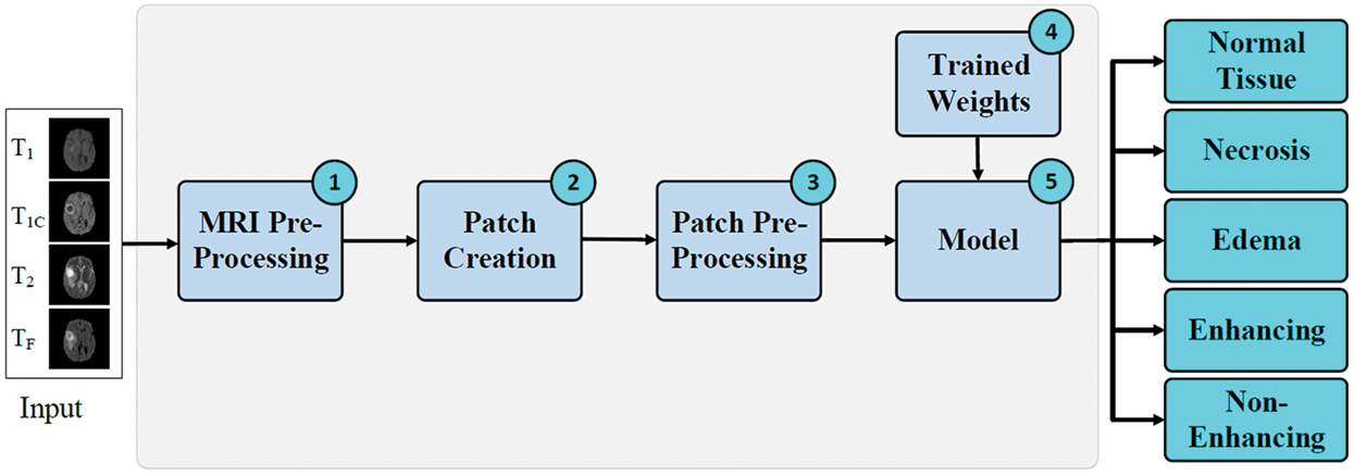
Figure 1: Proposed method for classification of enhancing tumor regions
The MRI scans usually have inherited noise due to the biased distortion field which cause the intensity variation in tissues across an image. The CNN’s models are normally noise-tolerant up to a certain level. Experiments have proved that if pre-processed data is provided to these models, they perform exceptionally well as compared to the un-processed data. The Probability Density Function (PDF) Of 2D MRI slices indicate the presence of Gaussian noise. So, in order to remove the Gaussian noise, we have employed the non-local means filter [32], as it performs very well for the Gaussian noise removal and preserve the edge information, which is very crucial for the segmentation task. Conventional local mean filters take the mean of pixels within the window. Whereas in non-local mean filter, the pixels having similar intensity values within a defined window are used for the mean calculation. The mathematical form of non-local mean filter [32] is given as:
where Ω is the image size, u(p) is the filtered value at point p of an image. Whereas v(q) is the original value at point q. The weighted function is given as f(p, q) and C(p) is the normalizing factor.
Once 2D slices of all modalities are pre-processed and noise is removed, 2D patches are created which are then used for training the CNN model. In order to create these patches, we used the 2D slices of all 4 modalities, namely T1, T1c, T2, FLAIR along with the ground truth. Next, we randomly search for the pixel with the value close to the ground truth value of the class. Once that ground truth value is found we crop a region around that pixel to extract the patch. The cropped region has the same size as of the ground truth patch. In our case, we used a moderate 31 × 31 patch size to accommodate variation in the tumor lesions. After region cropping as a patch, it is ensured that it must contain at least 50% of pixels of that class for which the patch is being created otherwise discard the patch and create a new one until the above condition is met.
The next step in the proposed methodology is pre-processing the created patches. The main goal of patch pre-processing is to achieve convergence faster in the training process. For that, we normalized the patches with zero mean and unit variance. As a result, the intensity values of all the patches lie between −1 and 1 which helps the CNN to converge faster. The patch normalization is done using the following equation.
where μ, σ represents the mean and standard deviation of patch x, respectively.
The pre-processed patches
The training weights are useful in boosting the prediction accuracy of the CNN model. They are used to help in predicting the class labels. In the proposed method, the CNN model is trained using 2D patches along with the associated ground truth patch. After training, the 10-fold cross-validation is applied to check the model performance on different cases. Once training is complete, the best trained weights are then saved. These trained weights are then used in step 5 of the proposed method to predict the class labels for each patch.
The class labels are predicted using a CNN model. The CNN model have been producing state-of-the-art results since their breakthrough in ImageNet Large Scale Visual Recognition Challenge (ILSVRC) [22]. The CNN’s are very similar to simple neural networks as they have neurons that are given inputs and in return, they produce some output. These neurons have trainable weights and biases. In CNN, there are convolutional layers in which inputs are convolved using a kernel, and as results feature maps are produced. In the training phase, the weights of kernels are adjusted when the error is back-propagated. Since connections are made sparsely in convolutional layers so there are fewer weights to train as compared to fully connected layers where dense connections are made. The purpose of kernels is to extract features from data such as edges or blotch of some colors. Variable size of kernels can be used, depending on the neighborhood and the amount of information required to learn [24,33,34].
In practice, convolutional layers are stacked on each other. Each convolutional layer extract features maps that gets abstract on layer after layer. A simple CNN contains convolutional layers, dense layers (FC layers), pooling layers, softmax layer, activation functions, loss function, and regularization parameters.
1) Initialization: Weight initialization is used to achieve convergence and to propagate signal through the network. For the initialization of weights, we use Xavier Initialization [35], given below.
2) Activation Function: The activation function in CNN produce an output of the node when it given some input. In our model, we have used a rectifier linear unit (ReLU) which performs better than traditional sigmoid or hyperbolic tangent functions. ReLU is defined as:
3) Pooling: Pooling is used for down-sampling in a CNN to reduce the computational load. In the pooling, we can use average pooling [9] or max-pooling depending on our needs. Pooling should not be used in starting layers as important information might be lost. In our model, we are using max pooling.
4) Regularization: Regularization is used in CNN during training to avoid over-fitting. In order to generalize overall training examples, we used regularization techniques to discard a certain amount of signal. In our model, we are using dropout [36,37] in dense and convolutional layers.
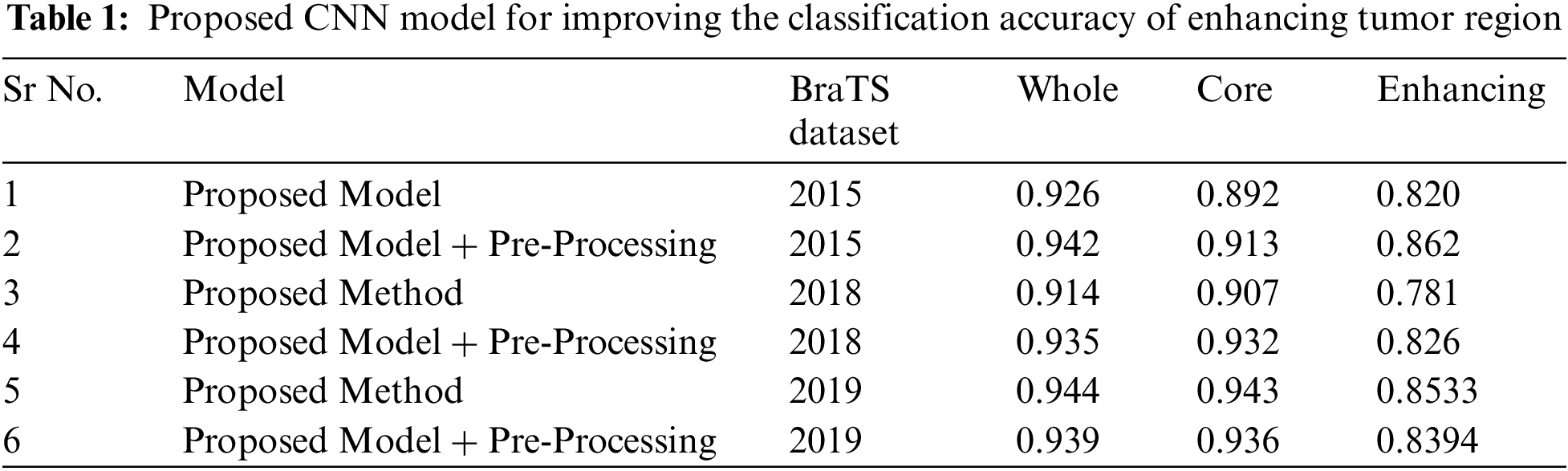
5) Architecture: Combination of convolutional, pooling, fully connected and softmax layers form a convolutional neural network. The table below shows the arrangement of layers and their configurations in order to build the proposed model for improving the class accuracy of enhancing the tumor region are shown is the Tab. 1 below.
3) Loss Function: Loss function calculates the difference between predicted value and the actual value (ground truth). We are using categorical cross-entropy as loss function for our model.
Here
5) Model Output: Finally, once the input patch is processed by the deep learning model, the class labels are produced from one of the five classes namely: normal, necrosis, edema, enhancing, and non-enhancing. Each class has a score between 0 and 1. The class having score higher than 0.5 is considered a positive prediction otherwise it is a negative prediction. The model can predict multiple labels at the same time.
In this section, we are presenting an insight into the dataset and study the significance of the proposed method by experimental evaluation. First, we discuss the configurations and hyper-parameters that are required for setting up the experiment. Later, we are going to talk about the metrics used to evaluate the performance of our classification model. Lastly, we will explain the results of our experiments in detail.
A. Dataset
The experiments are conducted on the BRATS 2015 training database [5,38]. BRATS dataset has both real patient data and synthetic data along with their ground truth. The dataset is divided into two parts Low-Grade Gliomas (LGG) and High-Grade Gliomas (HGG) with LGG being less aggressive than HGG. There are 220 samples of HGG and 54 samples of LGG. Each sample of the patient has four modalities namely T1, T1 Contrast (T1c), T2, and T2 FLAIR. In T1 modality, tissues with high-fat content appear bright and compartments filled with water appear dark. In T1c modality has high contrast in comparison to T1 modality other than that both modalities are similar. In T2 modality, compartments filled with water appear bright and high-fat content appears dark. Whereas, T2 FLAIR is similar to T2, but with comparatively longer Echo Time (TE) and Repetition Time (TR). First, we conduct experiments on HGG because samples of necrosis and enhancing tumor are small in the LGG dataset. Figs. 2a–2d gives a visual of all four MRI modalities.
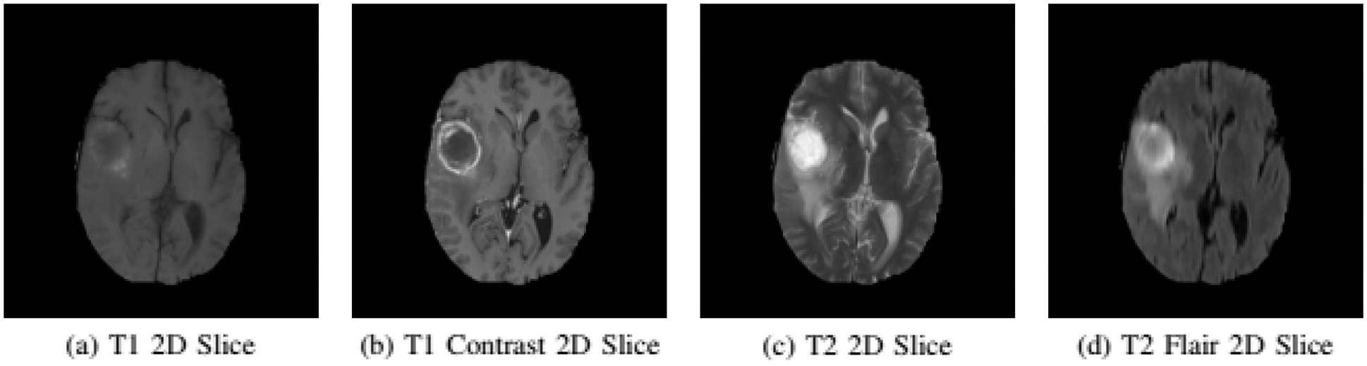
Figure 2: Imaging modalities in BRATS 2015 dataset
B. Setup
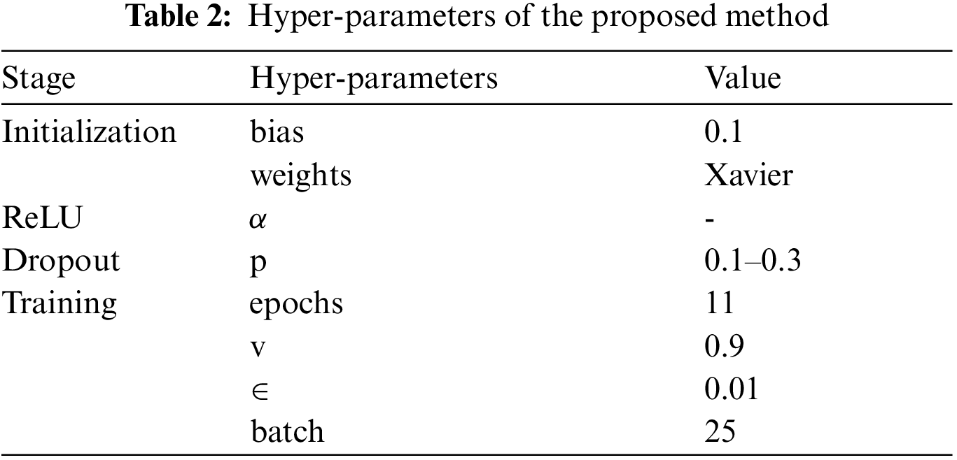
In order to replicate the experiment, the hyper-parameters setting of the model are given in Tab. 2. For training the model we extracted 125, 000 patches from the HGG samples of the BRATS dataset. The CNN model was developed using Keras [39] along with Tensorflow-GPU [40] back-end.
C. Example
In this section we are presenting an example of our proposed method. We will visualize the output of each step: 2D Slice Extraction, MRI Pre-Processing, 2D Patch Extraction, and 2D Patch Pre-Processing. The dataset used in this example is from BRATS 2015.1) 2D Slice Extraction: The 2D slices are extracted from the volumes of all four MRI modalities. Each 3D volume contains 155 slices. The extracted 2D slices can be seen in Fig. 3 along with their ground truth.
2) MRI Pre-Processing: The histograms of the 2D MRI slices of all 4 modalities indicate the presence of Gaussian noise. This Gaussian noise is mainly due to the intensity inhomogeneity problem in MRI scans. We have applied the non-local means filter on the 2D MRI slices. The denoising effect of non-local means filter can be seen in Fig. 4.
3) 2D Patch Extraction: We extracted equal number of patches for each tumor classes. The patches of each tumor class can be seen in Fig. 5. These patches are then used for the CNN model training.
4) 2D Patch Pre-Processing: The extracted patches are normalized so that the CNN classifier can converge faster and training process can speed up. For normalization of patches, we applied zero mean and unit variance to patches.
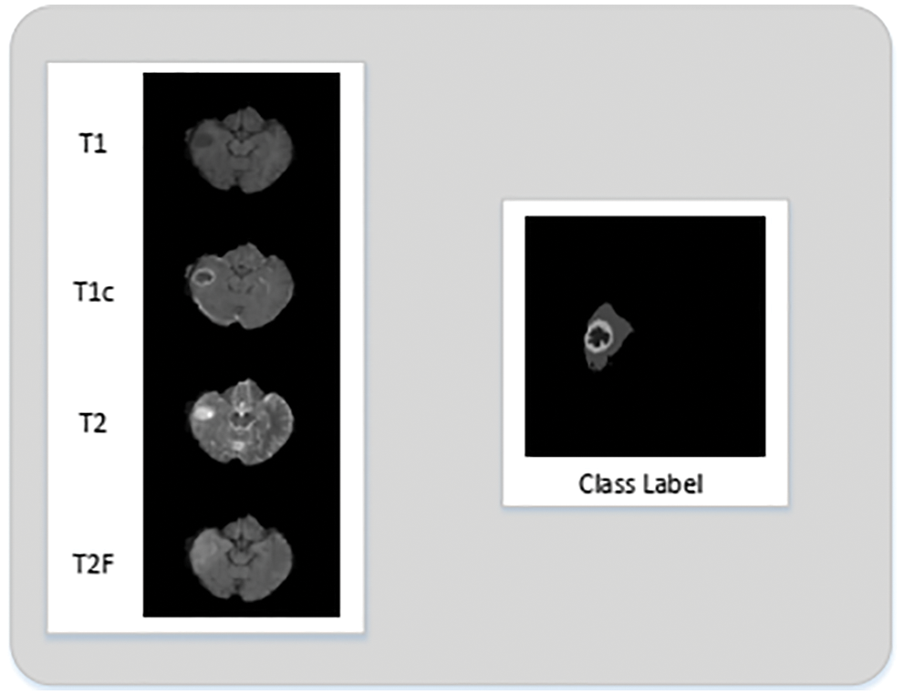
Figure 3: 2D slices extracted from MRI volume
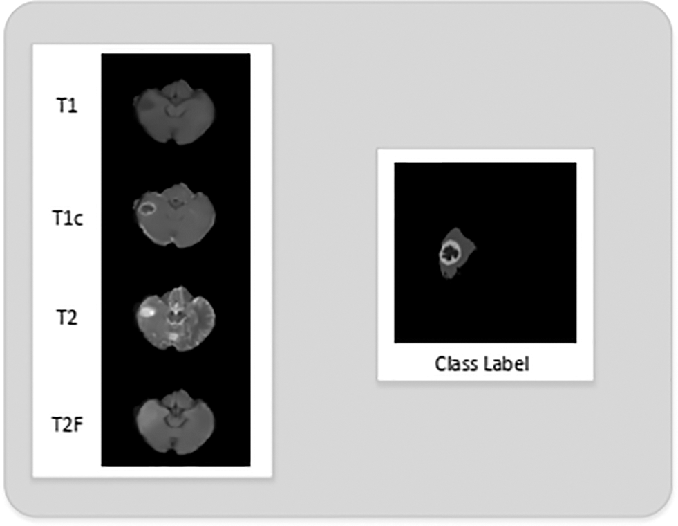
Figure 4: 2D slices of T1, T1c, T2 and T2 flair after non-local means filter is employed for denoising
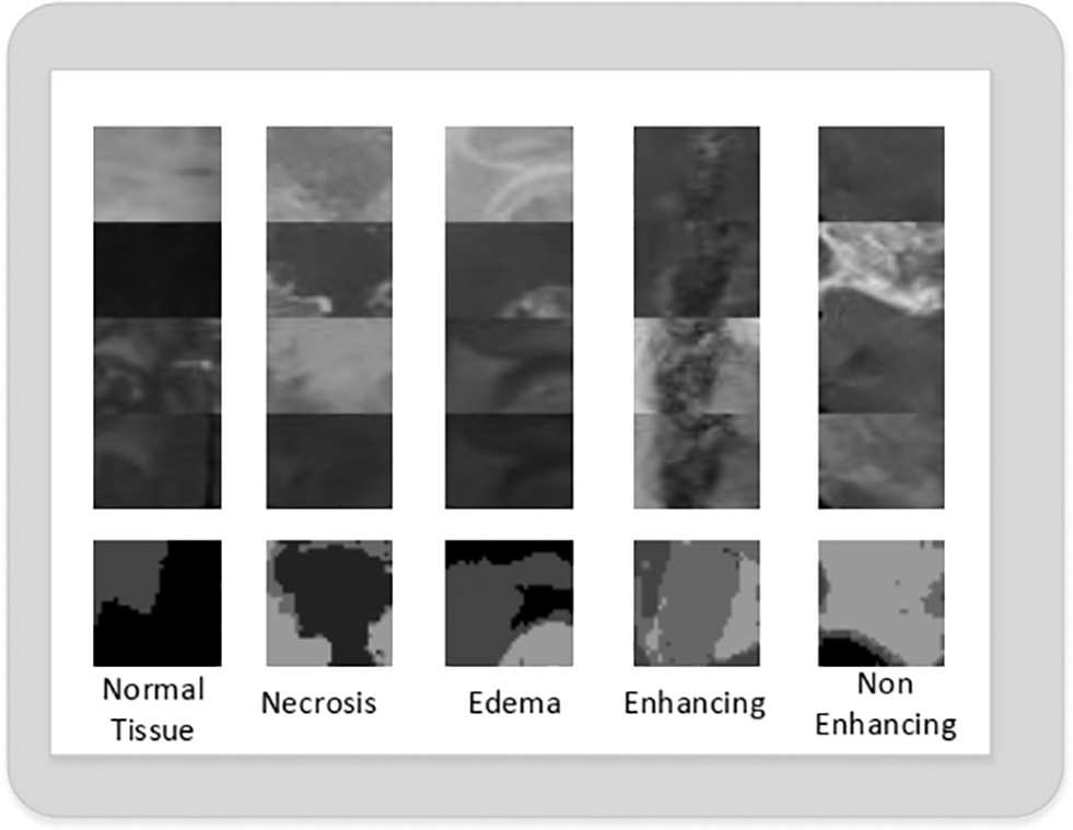
Figure 5: Extracted 2D patches of normal, necrosis, edema, enhancing and non-enhancing tumor class
D. Evaluation
Once the training phase is completed next comes the phase of evaluating the performance of the model. In order to do that the model needs to be evaluated on certain metrics. Accuracy alone cannot be used to compute a model’s performance as it has its own shortcomings. For evaluating our trained model, we used Dice Similarity Coefficient (DSC), Positive Predictive Value (PPV), Sensitivity, Negative Predictive Value (NPV), False Positive Rate (FPR), Recall and F-1 score. A brief introduction to these metrics is given below. Where True Positive (TP) is an outcome when the model correctly predicts the positive class. True Negative (TN) is when the model correctly predicts the negative class. False Positive (FP) is when the model incorrectly predicts the positive class. False Negative (FN) is when the model incorrectly predicts the negative class.
1) Dice Similarity Coefficient (DSC): This is used for comparison between two samples, given as
2) Positive Predictive Value (PPV) or Precision: It is the proportion of cases correctly identified as belonging to class c among all cases in which the classifier claims that they belong to class c given as:
3) Sensitivity: Sensitivity is the measure to evaluate actual positives identified as positive, given as:
4) Negative Predictive Value (NPV): It is the probability that the samples truly do not have disease, given as:
5) False Positive Rate (FPR): It is ratio between negative events wrongly categorized as positive; given by :
6) Recall: Recall is the proportion of cases correctly identified as belonging to class c among all cases that truly belong to class c given as:
7) F-1 Score: F1-Score is the harmonic average of the precision and recall, where an F1 score reaches its best value at 1 (perfect precision and recall) and worst at 0 which is given as:
E. Results
In this section, we are going to analyze the effect of key components on the experiment and discuss the acquired results. BRATS is a multi-class MRI dataset. We have employed the patch wise training for the CNN model instead of training the whole MRI scan. A comparison of accuracy and number of epochs for the training phase is presented in Fig. 6. To report the accuracy scores, we have trained the model for 12 epochs. As we can see, from the 1st epoch the training accuracy is in low 80’s whereas the validation accuracy is in the high 80’s. After the 5th epoch, we can see an increase in training and validation accuracy until the mid-90’s. From the 5th epoch onwards the trend of validation and training accuracy tends to get static with no further improvements. So, after the 12th epoch, we stop the model training as global minima are achieved and we do not want our model to over-fit the training data.
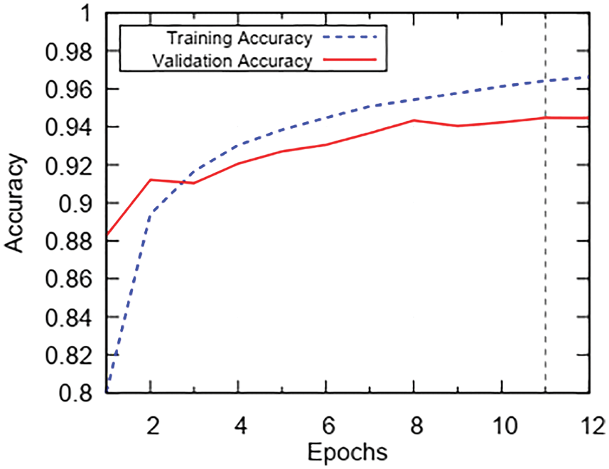
Figure 6: Trend of accuracy during 12 epochs of training
Now to check the loss trend during the training phase, we have trained the model for 12 epochs and the results are plotted in Fig. 7. We see that training loss starts at 0.55 and drops gradually until the 2nd epoch. After the 2nd epoch, the training loss keeps on decreasing slowly till 12th epoch and then training is stopped. Validation loss starts from 0.35 and gradually drops till the 2nd epoch. After the 2nd epoch validation loss sluggishly decreases to 0.19. After the 12th epoch, we stop training in order to prevent classifier from over-fitting training data. In Fig. 8, we present the classification report on metrics namely: Precision, Recall, and F-1 Score; on the x-axis and the tumor classes. The scores for enhancing tumor class are 0.94, 0.94, 0.94 for Precision, Recall and F1-Score; respectively. We have acquired impressive results for enhancing tumor class along with high Precision, Recall and F-1 Score for all the remaining classes as well. The obtained scores by the proposed method range between 0.91–0.98, which is in the high range for tumor classification.
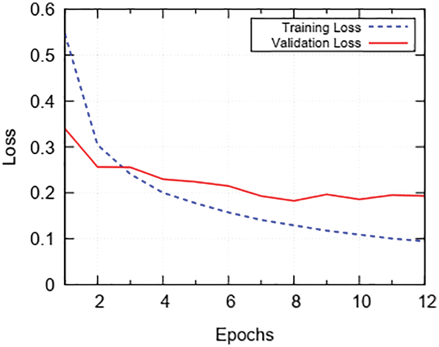
Figure 7: Trend of loss during 12 epochs of training
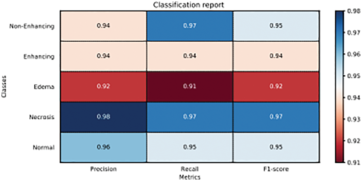
Figure 8: Classification report of proposed model on precision, recall and F1-score
It can be seen from the results shown in Figs. 6–8 that the trained model is performing very well on validation data but in order to examine predictive performance of the classifier new data or unseen examples of data needs to be given.
In order to check this, we employed K-Fold Cross-validation. The K-Fold cross-validation works as K-1 samples are used for training and the remaining 1 sample is used for validation. This process is repeated K times with each sample being used once as validation data. In this experiment, we used 10-Fold cross-validation. The DSC is used for comparison of the similarity between two samples. The performance of our proposed method on the DSC metric can be witnessed by looking at Tab. 3. In the table, we can see the average DSC score for all tumor classes on 10-Folds validation is 0.94. The average DSC score for enhancing tumor over the 10-Folds of validation is 0.93.
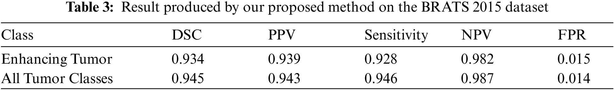
The sensitivity metric is used to check if the actual positives are identified as positive. In Tab. 3 we report the sensitivity value achieved by the proposed method. The average sensitivity score for all tumor classes is 0.94 over 10-Folds of validation. Whereas the average sensitivity score for enhancing tumor class is 0.92.
Similarly, in Tab. 3 we also presented the performance of our proposed CNN model on the Positive Predictive Value (PPV) metric. The purpose of the PPV metric is to check that the model predicts the true positives as positives. We can see that for all tumor classes the average PPV score is 0.94 for the 10-Folds of validation. For enhancing tumor class average PPV scores is 0.93 during 10-Folds of validation. The difference in the value is due to the variation in the sample examples.
Also, Tab. 3 shows the trend of Negative Predictive Value (NPV) over the 10 folds of cross validation. The purpose of NPV is to evaluate how accurately classifier can predict negative classes. We can see that average NPV scores remain in excess of 0.98 for all the classes. Our main objective was to increase the performance of enhancing tumor class and by looking at the table we observe that the scores for enhancing tumor class are very consistent as average NPV score stays around 0.98. Next, we look at the False Positive Rate (FPR) trend. The purpose of FPR is to check the percentage of false labels assigned to a sample during the testing phase. In Tab. 3 we can see that the FPR score is low for all tumor classes. The average score lies around 0.014. For enhancing tumor class, the average score remains around 0.01517 through entire 10 folds of validations.
The main goal of this work is to devise an automatic classification method for the enhancing tumor class, with improved accuracy. Also, the method should be able to achieve higher accuracies for all the other tumor classes as well. This is a challenging task due to the complex symmetry and variable shape of brain structure. Secondly, the enhancing tumor class has a low classification accuracy due to the fact that these tumors are in their initial phases of growth and appear dark on MRI which makes them difficult to identify.
In the proposed solution we have improved the classification accuracy for enhancing tumor class. This was mainly achieved by applying a pipeline of pre-processing, a customized CNN classifier followed by the post processing. We observed that the PDF of MRI scans possess Gaussian noise and in order to remove that we applied non-local mean filters [32]. After MRI was pre-processed, we then created 2D slices from the 3D volumes of MRI. The reason for using 2D slices was because training a model with 3D voxels is computationally very expensive. The extracted patches were from the axial plane. Once the 2D patches were created they were then pre-processed to normalize to achieve faster convergence during the training of CNN model. Last, the pre-processed patch was given as input to the model which in return predicted the class labels for the given patch.
For training the model we did MRI pre-processing, patch extraction, patch pre-processing and tuning of training weights for CNN model. The model was trained for 12epochs and 10-fold cross-validation was applied to check CNN model performance on easy and hard examples. Once 10-folds of cross-validation was completed the best weights were saved and used in the model for prediction of class labels. Once training of the model is completed and model is predicting class labels. The next step was evaluating the performance of CNN model. For evaluation accuracy alone cannot be used as it comes with its own shortcomings. Due to this reason, we have used Dice Similarity Coefficient (DSC), Specificity, Negative Predictive Value (NPV), False Positive Rate (FPR), Precision, Recall, and F-1 Score to evaluate the performance of the CNN model. The reported scores for all the metrics that are used to evaluate the model were not only impressive for enhancing tumor class but also for all the other tumor classes. The problem of classification accuracy for enhancing tumor region was eradicated by using small patches of the 31 × 31 size which was small enough to represent a class. Secondly, we ensured that the created patches for a certain class must contain 50% pixels of that class in the patch. Due to this novelty, the accuracy massively increased for enhancing tumor class and for other classes as well. We also used equal samples for all classes during the training phase which also eradicates the problem of class imbalance and eventually prevents classier from making biased predictions.
The objective of this research was to devise an automatic method that would be able to improve the classification accuracy for enhancing tumor region without degrading the accuracy of other tumor classes. For this purpose, we proposed an automatic classification method based on CNN model that enabled us to increase the classification accuracy of enhancing tumor region along with that it also achieved high classification scores for other tumor classes as well.
Future work that can be carried out for incremental research can be by doing segmentation from these classifications. Besides this different model e.g., U-nets or V-nets, with a slight variation can be employed to improve the prediction confidence for a larger dataset.
Funding Statement: The authors received no specific funding for this study.
Conflicts of Interest: The authors declare that they have no conflicts of interest to report regarding the present study.
1. Adult central nervous system tumors treatment. [Online]. Available: https://www.cancer.gov/types/brain/patient/adultbrain-treatment-pdqsection/all. [Google Scholar]
2. S. Bauer, R. Wiest, L. -P. Nolte and M. Reyes, “A survey of mri-based medical image analysis for brain tumor studies,” Physics in Medicine and Biology, vol. 58, no. 13, pp. 97–103, 2013. [Google Scholar]
3. D. N. Louis, H. Ohgaki, O. D. Wiestler, W. K. Cavenee, P. C. Burger et al., “The 2007 WHO classification of tumours of the central nervous system,” ACTA Neuropathologica, vol. 114, no. 2, pp. 97–109, 2007. [Google Scholar]
4. E. G. Van Meir, C. G. Hadjipanayis, A. D. Norden, H. -K. Shu, P. Y. Wen et al., “Exciting new advances in neuro-oncology: The avenue to a cure for malignant glioma,” CA: A Cancer Journal for Clinicians, vol. 60, no. 3, pp. 166–193, 2010. [Google Scholar]
5. B. H. Menze, A. Jakab, S. Bauer, J. Kalpathy-Cramer, K. Farahani et al., “The multimodal brain tumor image segmentation benchmark (BRATS),” IEEE Transactions on Medical Imaging, vol. 34, no. 10, pp. 1993–2024, 2015. [Google Scholar]
6. N. J. Tustison, B. B. Avants, P. A. Cook, Y. Zheng, A. Egan et al., “N4itk: Improved n3 bias correction,” IEEE Transactions on Medical Imaging, vol. 29, no. 6, pp. 1310–1320, 2010. [Google Scholar]
7. L. G. Nyul, J. K. Udupa and X. Zhang, “New variants of a method of mri scale standardization,” IEEE Transactions on Medical Imaging, vol. 19, no. 2, pp. 143–150, 2000. [Google Scholar]
8. S. Pereira, A. Pinto, V. Alves and C. A. Silva, “Brain tumor segmentation using convolutional neural networks in MRI images,” IEEE Transactions on Medical Imaging, vol. 35, no. 5, pp. 1240–1251, 2016. [Google Scholar]
9. Y. LeCun, Y. Bengio and G. Hinton, “Deep learning,” Nature, vol. 521, no. 7553, pp. 436–444, 2015. [Google Scholar]
10. R. Meier, S. Bauer, J. Slotboom, R. Wiest and M. Reyes, “Appearance-and context-sensitive features for brain tumor segmentation,” Proceedings of MICCAI BRATS Challenge, Boston, USA, pp. 20–26, 2014. [Google Scholar]
11. D. Zikic, B. Glocker, E. Konukoglu, A. Criminisi, C. Demiralp et al., “Decision forests for tissue-specific segmentation of high-grade gliomas in multi-channel MR,” in Int. Conf. on Medical Image Computing and Computer-Assisted Intervention, Nice, France, Springer, 2012, pp. 369–376. [Google Scholar]
12. A. Pinto, S. Pereira, H. Correia, J. Oliveira, D. M. Rasteiro et al., “Brain tumour segmentation based on extremely randomized forest with high-level features,” in Engineering in Medicine and Biology Society (EMBCAnnual Int. Conf. of the IEEE, Milan, Italy, 2015, pp. 3037–3040. [Google Scholar]
13. R. Meier, S. Bauer, J. Slotboom, R. Wiest and M. Reyes, “A hybrid model for multimodal brain tumor segmentation,” Multimodal Brain Tumor Segmentation, vol. 31, pp. 1993–2024, 2013. [Google Scholar]
14. S. Reza and K. Iftekharuddin, “Multi-fractal texture features for brain tumor and edema segmentation,” SPIE Medical Imaging. International Society for Optics and Photonics, pp. 503–903, 2014. [Google Scholar]
15. A. Islam, S. M. Reza and K. M. Iftekharuddin, “Multifractal texture estimation for detection and segmentation of brain tumors,” IEEE Transactions on Biomedical Engineering, vol. 60, no. 11, pp. 3204–3215, 2013. [Google Scholar]
16. N. J. Tustison, K. Shrinidhi, M. Wintermark, C. R. Durst, B. M. Kandel et al., “Optimal symmetric multimodal templates and concatenated random forests for supervised brain tumor segmentation (simplified) with antsr,” Neuroinformatics, vol. 13, no. 2, pp. 209–225, 2015. [Google Scholar]
17. S. Bauer, L. -P. Nolte and M. Reyes, “Fully automatic segmentation of brain tumor images using support vector machine classification in combination with hierarchical conditional random field regularization,” in Int. Conf. on Medical Image Computing and Computer-Assisted Intervention, Toronto, Canada, Springer, 2011, pp. 354–361. [Google Scholar]
18. C. -H. Lee, S. Wang, A. Murtha, M. R. Brown and R. Greiner, “Segmenting brain tumors using pseudo–conditional random fields,” in Int. Conf. on Medical Image Computing and Computer-Assisted Intervention, New York City, USA, Springer, 2008, pp. 359–366. [Google Scholar]
19. E. Geremia, B. H. Menze and N. Ayache, “Spatially adaptive random forests,” in IEEE Int. Symp. on Biomedical Imaging (ISBI), San Francisco, CA, USA, pp. 1344–1347, 2013. [Google Scholar]
20. R. Meier, S. Bauer, J. Slotboom, R. Wiest and M. Reyes, “Patient-specific semi-supervised learning for postoperative brain tumor segmentation,” in Int. Conf. on Medical Image Computing and Computer-Assisted Intervention, Cambridge, United States, Springer, 2014, pp. 714–721. [Google Scholar]
21. A. Krizhevsky, I. Sutskever and G. E. Hinton, “ImageNet classification with deep convolutional neural networks,” Communications of the ACM, vol. 60, pp. 84–90, 2017. [Google Scholar]
22. S. Dieleman, K. W. Willett and J. Dambre, “Rotation-invariant convolutional neural networks for galaxy morphology prediction,” Monthly Notices of the Royal Astronomical Society, vol. 450, no. 2, pp. 1441–1459, 2015. [Google Scholar]
23. D. Ciresan, A. Giusti, L. M. Gambardella and J. Schmidhuber, “Deep neural networks segment neuronal membranes in14 electron microscopy images,” Advances in Neural Information Processing Systems, vol. 25, pp. 2843–2851, 2012. [Google Scholar]
24. D. Zikic, Y. Ioannou, M. Brown and A. Criminisi, “Segmentation of brain tumor tissues with convolutional neural networks,” Proc. MICCAI-BraTS, Cambridge, United States, pp. 36–39, 2014. [Google Scholar]
25. G. Urban, M. Bendszus, F. Hamprecht and J. Kleesiek, “Multi-modal brain tumor segmentation using deep convolutional neural networks,” MICCAI BraTS Challenge. Proc. Winning Contribution, Cambridge, US, pp. 31–35, 2014. [Google Scholar]
26. M. Havaei, A. Davy, D. Warde-Farley, A. Biard, A. Courville et al., “Brain tumor segmentation with deep neural networks,” Medical Image Analysis, vol. 35, pp. 18–31, 2017. [Google Scholar]
27. M. Lyksborg, O. Puonti, M. Agn and R. Larsen, “An ensemble of 2d convolutional neural networks for tumor segmentation,” in Scandinavian Conf. on Image Analysis, Copenhagen, Denmark, Springer, 2015, pp. 201–211. [Google Scholar]
28. V. Rao, M. Sarabi and A. Jaiswal, “Brain tumor segmentation with deep learning,” Proc. MICCAI-BraTS, Munich, Germany, pp. 56–59, 2015. [Google Scholar]
29. P. Dvorak and B. Menze, “Structured prediction with convolutional neural networks for multimodal brain tumor segmentation,” Proc. MICCAI-BraTS, Munich, Germany, pp. 13–24, 2015. [Google Scholar]
30. P. Dvorak and B. Menze, “Local structure prediction with convolutional neural networks for multimodal brain tumor segmentation,” in Int. MICCAI Workshop on Medical Computer Vision, Munich, Germany, Springer, 2015, pp. 59–71. [Google Scholar]
31. K. Simonyan and A. Zisserman, “Very deep convolutional networks for large-scale image recognition,” arXiv preprint arXiv:1409.1556, 2014. [Google Scholar]
32. A. Buades, B. Coll and J. -M. Morel, “A Non-local algorithm for image denoising,” in IEEE Conf. on Computer Vision and Pattern Recognition, San Diego, CA, USA, vol. 2, pp. 60–65. 2005. [Google Scholar]
33. Y. LeCun, B. Boser, J. S. Denker, D. Henderson, R. E. Howard et al., “Backpropagation applied to handwritten zip code recognition,” Neural Computation, vol. 1, no. 4, pp. 541–551, 1989. [Google Scholar]
34. Y. LeCun, L. Bottou, Y. Bengio and P. Haffner, “Gradient-based learning applied to document recognition,” Proceedings of the IEEE, vol. 86, no. 11, pp. 2278–2324, 1998. [Google Scholar]
35. X. Glorot and Y. Bengio, “Understanding the difficulty of training deep feedforward neural networks,” in Proc. of the Thirteenth Int. Conf. on Artificial Intelligence and Statistics, Sardinia, Italy, pp. 249–256, 2010. [Google Scholar]
36. N. Srivastava, G. E. Hinton, A. Krizhevsky, I. Sutskever and R. Salakhutdinov, “Dropout: A simple way to prevent neural networks from overfitting.” Journal of Machine Learning Research, vol. 15, no. 1, pp. 1929–1958, 2014. [Google Scholar]
37. G. E. Hinton, N. Srivastava, A. Krizhevsky, I. Sutskever and R. R. Salakhutdinov, “Improving neural networks by preventing co-adaptation of feature detectors,” arXiv preprint arXiv:1207.0580, 2012. [Google Scholar]
38. M. Kistler, S. Bonaretti, M. Pfahrer, R. Niklaus and P. Buchler, “The virtual skeleton database: An open access repository ¨ for biomedical research and collaboration,” Journal of Medical Internet Research, vol. 15, no. 11, pp. e245, 2013. [Google Scholar]
39. F. Chollet, “Keras,” https://keras.io, 2015. [Google Scholar]
40. M. Abadi, P. Barham, J. Chen, Z. Chen, A. Davis et al., “Tensorflow: A system for large-scale machine learning.” in Proc. of the 12th USENIX Conf. on Operating Systems Design and Implementation, Savannah, GA, USA, vol. 16, pp. 265–283, 2016. [Google Scholar]
 | This work is licensed under a Creative Commons Attribution 4.0 International License, which permits unrestricted use, distribution, and reproduction in any medium, provided the original work is properly cited. |