DOI:10.32604/cmc.2022.026070
| Computers, Materials & Continua DOI:10.32604/cmc.2022.026070 | |
| Article |
An Efficient Path Planning Strategy in Mobile Sink Wireless Sensor Networks
Department of Computer Science, Faculty of Computing and Information Technology, King Abdul-Aziz University, Jeddah, 21589, Saudi Arabia
*Corresponding Author: Najla Bagais. Email: najlabagias.resercher@gmail.com
Received: 14 December 2021; Accepted: 02 March 2022
Abstract: Wireless sensor networks (WSNs) are considered the backbone of the Internet of Things (IoT), which enables sensor nodes (SNs) to achieve applications similarly to human intelligence. However, integrating a WSN with the IoT is challenging and causes issues that require careful exploration. Prolonging the lifetime of a network through appropriately utilising energy consumption is among the essential challenges due to the limited resources of SNs. Thus, recent research has examined mobile sinks (MSs), which have been introduced to improve the overall efficiency of WSNs. MSs bear the burden of data collection instead of consuming energy at the routeing by SNs. In a network, some areas generate more data through SNs that contain frequent, urgent messages. These messages carry sensitive data that must be delivered immediately to user applications. Collecting such messages via MSs, especially on a large scale, increases delays, which are not tolerable in some real applications. This issue has not been studied much. Thus, the present study utilises the advantages of the priority parameter to concentrate on these areas and proposes a new model named ‘energy efficient path planning of MS-based area priority’ (EEPP-BAP). This method involves non-urgent and urgent messages. It is comprised of four procedures. Initially, after SNs are distributed randomly in a wide monitoring field, the monitoring field is partitioned into equal zones according to priority, either differently or equally. Next is clustering based on the cluster head (CH) selected to perform the particle swarm optimisation algorithm (PSO). Then, the MS moves first to the zones with higher priority and less distance to perform the brain storm optimisation algorithm. Finally, for urgent messages from the other zones at which the MS continues, the proposed approach establishes a routeing technique using multi-hop communication based on the MS position and using PSO. The proposed solution is aimed at delivering urgent messages to MSs free of latency and with minimal packet loss. The simulation results proved that the EEPP-BAP method can improve network performance compared with other models based on different parameters that have been used to construct the controlled movement of MSs in large-scale environments involving urgent messages. The proposed method increased the average lifetime of SNs to 206.6% on average, reduced the average end-to-end delay to 7.1%, and increased the average packet delivery ratio to 36.9%.
Keywords: Wireless sensor network; priority; urgent message; swarm intelligence optimisation; mobile sink; clustering; energy efficiency
Recently, wireless technology communication has been considered an essential means of enabling users to communicate via a wide range of applications, including animal monitoring, fire detection, agriculture monitoring, and medical and military applications, using wireless sensor networks (WSNs) [1,2]. A WSN can be described as a group of tiny devices called sensor nodes (SNs) that are connected through wireless communication to sense data from the surrounding environment and then transmit them to a static sink node or base station via a multi-hop communication network. In some applications, SNs are distributed randomly in the coveted area for tracking or monitoring. A WSN can use full, partial, or isolated connections based on the scale of the area in which the SNs are deployed.
WSNs are considered a pillar of the Internet of Things (IoT), as SNs support mobile applications through remote communication. The IoT allows devices, objects, and people to communicate and interact in the network without intermediate human intervention, bringing the IoT intelligence and automation to daily life. The integration of WSNs with the IoT authorises SNs to dynamically link with the Internet for cooperation, as illustrated in a simplified scenario depicted in Fig. 1. In the first layer, SNs sense the required data in a particular field and then wirelessly route or transmit the data to the static sink or MS. Next, at the transmission layer, the sink exchanges data via the Internet to a cloud platform. The sink can execute data sensing using its unlimited resources. The last stage is the application layer, which represents the end user and final decisions regarding the data [3].

Figure 1: Scenario depicting simplified layers of integrated WSNs in the IoT
However, the integration of WSNs with the IoT includes challenges, such as latency, reliability, and energy efficiency, due to the enormous areas of application across different technologies using different devices, which are increasing annually [4]. The energy usage of SNs represents the main research concern because of the limited resources from their main energy supply, batteries [4]. SNs consume the highest amount of energy during communication. Thus, SNs near the static sink node are at risk of dying more quickly than those at other nodes. As Fig. 2 illustrates, SNs drain extra energy to route accumulative data to a static sink node, causing hot spot problems.

Figure 2: Hot spot problems in WSNs with static sinks
Hot spot problems isolate other SNs, which in turn affects the monitoring area connectivity, preventing the SNs from transmitting data to a static sink node. Consequently, the network lifetime decreases. Furthermore, recharging SN batteries is often difficult, especially in hazardous or inaccessible areas. Thus, the primary research considerations in this field involve the energy consumption of SNs to maximise their operation and thereby extend their network lifespans [5].
The clustering technique has been applied widely in WSNs owing to its efficiency in preserving energy. The clustering method groups the SNs in a network into multiple clusters. At each cluster, a head node, named the cluster head (CH), is selected. The CH manages the cluster and collects data from SNs within the cluster, called cluster members (CMs) [6].
Although the clustering technique has been used in research for energy-efficient schema that contributes to prolonging the network life by minimising large-scale distance, improving connectivity, increasing reliability, and balancing energy usage, the hot spot and connectivity problems remain [7]. Therefore, a mobile sink (MS) has been suggested as one way of resolving the energy consumption problem of WSNs. As illustrated in Fig. 3, an MS can move near SNs via the path planning method, which schedules the MS movements and collects the required data from SNs instead of utilising static sink nodes.

Figure 3: WSN using a mobile sink
As a result, the energy of the nodes is conserved by minimising the distances between the SNs and the MS. This model also reduces multi-hop communications and alleviates hot spot problems, enhancing the network lifetime [8].
Implementing path planning for MSs refers to finding the optimal path between SNs for data collection. The path planning problem is considered a ‘hard optimisation’ problem; the problem can be formulated in several ways based on the specifications of the applications involved. This type of problem can be solved by utilising stochastic-meta-heuristic algorithms more successfully than any other methods such as deterministic algorithms [9].
Meta-heuristic algorithms are inspired by the nature of some species based on populations. Evolutionary algorithms and swarm intelligence optimisation algorithms (SIO) are meta-heuristic algorithms that have been applied to solve the problem of MS path planning in WSNs. These algorithms have been an area of recent concentration for research on WSN optimisation issues such as localisation and routeing [10].
In a WSN, MSs have three primary movement patterns: random, controlled, and uncontrolled [11].
• Random: The MS can be a device attached to a mobile element. The mobile element moves randomly in the sensing field without advance knowledge of or control over the direction and speed of movement in an animal-like manner. In addition, this pattern has a low scheduling prediction rate. It is viable for applications that are insensitive to delays [12].
• Controlled: The MS can be a device attached to mobile elements such as vehicles and robots. The mobile element moves in the sensing field completely controlled by the users. The user controls and adapts the direction, speed, and scheduling based on the purpose of the application [13].
• Uncontrolled: This is also called a ‘predictable mobility pattern’, in which the MS can be a device attached to a mobile element such as a MS. The MS always moves in the sensing field on a certain fixed path, like a train or bus. The speed, direction, scheduling, and routeing are defined in advance by the users. In addition, the SNs anticipate the visiting time of the mobile element [14].
From among these three movement patterns, research considers the controlled movement pattern because it can optimise the main issue of mobile element path planning in terms of speed, direction, and scheduling [15].
However, some MS applications involve on-demand needs such as urgent messages in some areas that should be delivered immediately to the MS position. The MS movement via fixed path planning to collect data from certain SNs without considering their residual energy leads to energy imbalances among all SNs in the network. Thus, these SNs are vulnerable to early death. In addition, a fixed MS path may cause data packets to be dropped by SNs that carry urgent messages because of their limited buffer size. In addition, when data are urgently required to arrive instantly at the end user, SNs waiting with urgent messages until the MS arrives cause unacceptable delays that make the time-sensitive data useless [15].
Path planning of MS-controlled movement patterns involves parameters that have been underexplored in previous studies, including area priority and on-demand needs such as routeing urgent messages to the position of an MS. ‘Area priority’ refers to the sub-areas in the network that are most likely to contain urgent messages that require immediate delivery to the MS or end user. ‘On-demand’ refers to the need to immediately deliver sensitive data regarding unexpected events occurring within the monitoring area, such as a fire event. Therefore, a more efficient path planning model is needed for MSs to consider more parameters that enable the system to maximise the lifetime of SNs, minimise delays, and reduce packet loss [15].
Handling these parameters can extend the network lifetime, reduce delays, and improve readability. In the case of area priority, SNs with urgent messages within the sub-area of priority can minimise the routeing distance to the MS position and can even avoid extensive rerouting to the MS in the network. Another parameter is routeing urgent messages, in which SNs are instructed to deliver urgent messages to the MS position immediately when they appear in the network.
Thus, this research contributes the following to the field:
• A method named ‘energy efficient path planning of MS-based area priority’ (EEPP-BAP) for utilising two parameters: area priority and routeing urgent messages to the MS position in WSN.
• Adaption of the particle swarm optimisation (PSO) algorithm for CH selection.
• Adaptation of the brain storm optimisation (BSO) algorithm to construct a MS path plan, with consideration of the priority and distance in the fitness function formulation.
• Adaptation of the PSO algorithm to establish a dynamic routeing technique for urgent messages that accounts for the current MS position.
The PSO and BSO algorithms have been carefully chosen due to their efficiency in many WSN applications, as in several prior studies [16–18]. Moreover, PSO performs much better than other algorithms in dynamic environments that require prompt responses to events and involve minimal computation [19].
PSO is a SIO that mimics the behaviour of a swarm such as birds flocking to find food or shelter; in other words, the flocking concept is used to find the best solution or global solutions in each generation or iteration. In each generation, potential solutions, called particles, become candidates for the next generation and are evaluated by the fitness function. They travel together as a group and follow each other at the same velocity and position, exchanging their information with each other to adjust without collisions. Each particle saves its better solution and follows the particle that has the best solution. This process facilitates finding food or shelter as a group instead of one individual exhausting its efforts alone [20].
The BSO algorithm is a swarm algorithm that mimics humans' brainstorming processes to solve a complex problem. BSO captures the essential factors in its exploration and exploitation to find solutions called ideas. In its exploration, it uses a global search to explore potential areas containing promising ideas in the entire search space within the domain of the problem. In addition, convergence and divergence are the two important processes in the BSO algorithm. During convergence, solutions are grouped into clusters, from the initial random ideas distributed across the search space domain. Divergence generates new individuals in the population from the clusters through mutation [21]. These two algorithms were used in this research and are presented briefly herein.
The rest of this research is organised as follows: Section 2 presents a review of the relevant literature and related work. Section 3 explains the proposed EEPP-BAP framework, and Section 4 simulates the proposed EEPP-BAP. Section 5 provides the performance evaluation, including the performance metrics and results. Finally, Section 6 discusses the conclusions, suggestions for future work, findings, and conflicts of interest.
Many studies have concentrated on energy efficiency in WSNs with stationary SNs and MSs to prolong network lifetime. This section presents recent studies on WSNs using MSs. These studies are categorised using cluster- and rendezvous point (RP)-based approaches, in which artificial intelligence (AI) algorithms are utilised to build optimised solutions in WSNs. These are followed by two studies that used a flat-based approach. These methods utilise priority parameters. Then, the problems that persist in WSNs with MSs are discussed.
2.1 Research on MS Path Planning Based on Clustering
Prior research has used the clustering approach in WSNs such that each collection of SNs is grouped into clusters. Each cluster has a CH that collects data from the SNs in that cluster. Then, an MS path is planned to visit each CH to collect sensor data. Most clustering algorithms are commonly known as the improved K-means clustering algorithm.
The energy-efficient algorithm based on the bacterial foraging optimisation algorithm (SMBFOA) is presented in one research [22] to address the throughput and energy conservation problems in the clustering duty cycle mobility-aware protocol algorithm. Authors [23] have proposed an efficient path for MS-based clustering. The same authors used the MS as an autonomous unmanned aerial vehicle (UAV) to gather data from CHs conducting water area monitoring. The main concern was to conserve UAV energy by reducing the path length via ant colony optimisation (ACO). To further reduce the MS path, the bisection method was applied after ACO to find the best stopping points. These points are located at the edge of the communication range of each CH. In another study [24], researchers proposed the use of the ACO algorithm with dynamic clustering to allow the construction of a shorter path among CHs to collect data in an acceptable length of time. A previous research [25] proposed the use of the evolutionary game-based trajectory design algorithm (EGTDA) for MS path planning to solve the energy imbalance that causes the hot spot problem. This algorithm considers the average residual energy in each cluster, that is, the average intra- and inter-cluster energy consumption. In addition to energy efficiency, many researchers have focused on reducing the MS path length to collect data. Furthermore, researchers have investigated other factors to improve path planning, such as throughput and obstacles. Another research project [26] divided data gathering in WSNs with obstacles (DGOB) into two phases: CH selection and construction of a shorter path between two CHs with obstacles between them. A study in [27] proposed an algorithm for inter-and intra-cluster movement of multi-mobile sinks in order to address unbalanced energy depletion among CHs and CMs, as well as provide solutions to the coverage hole problem. This algorithm improves the network performance by optimizing multiple sojourn locations in each cluster with respect to the time limitation for MSs movement using two stages (GA). Thus, the energy distributes evenly between CHs and CMs and the coverage hole is alleviated. The energy-efficient intra-cluster routing (EIR) with MS is proposed in [28] to balance the energy depletion among CMs within clusters. A formulation of this algorithm optimizes the selection of many sojourn locations within a cluster with constrained sojourn times. The movement of MS across these locations is optimized by applying (GA).
2.2 Research on MS Path Planning Based on RPs
Some studies have used the RP approach to conserve energy at RPs, which depend mainly on the MS in a WSN. RPs are the locations where the MS can visit to collect data in a cluster via multi-hop communication with long-term buffering. In this approach, no CHs are selected, only RPs [29].
In another study, authors have proposed a balancing inter- and inner-cluster energy (BIIE) algorithm for energy-balanced data collection between SNs under a constrained MS path in a WSN [29]. An efficient path planning algorithm is presented in an additional research [30] for multiple MSs, based on single-hop data collection in the disjointed area of a WSN. Each segment is isolated and consists of SNs and RPs that the MS visits, considering the MS path length constraints in each sub-tour. The main objectives of the research were to optimise the number and location of RPs and the number of MSs to collect all data via the minimum path-planning length to avoid latency. An energy-efficient trajectory planning (EETP) algorithm has been proposed [31] for an efficient path-planning algorithm to conserve energy in the MS and prolong the lifetime of network RNs through loading balance. A variable length genetic algorithm (VL-GA) was presented in the previous research [32] to optimise the number and location of RPs to shorten the MS path length to avoid delay and congestion buffering in SNs while waiting for the MS to arrive. The MS path planning algorithm, called the hexogen hyper-practical swarm optimisation (hexHPOS) algorithm, was further proposed [33] to balance the energy in each grid to improve network lifetime. An MS path planning method based on RPs, called priority-based distribution load-balancing clustering dual data uploading, has also been proposed [34] for data collection in WSNs to enhance energy consumption through load balancing and minimise latency in data delivery. The priority is assigned to SNs depending on the residual energy for each SN, and then the clustering priority is initialised. The SNs in a cluster transmit data to CHs through multi-hop communication. These CHs are covered by RPs, which receive data from the CHs.
Two previous studies [35,36] were flat-based, which means that each SN sends its messages to the MS via single- or multi-hop communication. These studies focused on different uses of priority without using an AI algorithm to construct the MS path plan.
The first research [35] proposed a differentiated message delivery (DMD) method to gather urgent and non-urgent messages via a controlled MS in a WSN. The SNs are grouped into bins and sub-bins (zones) according to deadline and location. The priority of visiting SNs is then based on the overflow time of the bins. The MS visits each SN in a bin simultaneously. Some sub-bins are visited in each cycle, while others are visited in alternating cycles. In this method, urgent messages rarely occur. Thus, a SN with urgent messages establishes a multi-hop routeing into the neighbouring SN in a bin that the MS visits frequently. This approach minimises the loss rate and improves the speed of the MS in a small monitoring field.
The second research proposed a framework for data gathering by an UAV as the uncontrolled MS, according to priority in a WSN [36]. During the movement of the UAV, some SNs in the rare areas of the UAV coverage are exposed to loss of UAV links. Therefore, the loss packet rate increases. Thus, according to the locations of the SNs in the UAV coverage area, the SNs are divided into various frames. Frames have various transmission priorities, with the rare regions in the UAV coverage area having the highest priority and the SNs in front of the UAV having the lowest priority. Thus, this approach minimises duplicate data and the loss rate and maximises throughput in a medium-sized monitoring field.
Tab. 1 presents a summary of the previous studies regarding their data collection algorithm schema for MS path planning and their different optimisation parameters. The optimisation parameters were as follows:
• Energy consumption: Almost all studies have taken into consideration SN energy because batteries only hold a limited amount of power. If SN energy consumption is not optimised properly, then the network is exposed to potential rapid death.
• MS path distance: This refers to the distance between the MS and the SNs during data transmission from an SN to the MS. When the distance increases, SNs consume more energy during transmission. Thus, most research has considered this parameter because of the effects of distance on SN lifetime.
• Message delay/latency: This refers to the time packets take to arrive at the sink location, either static or mobile. This parameter measures performance in terms of the time in delivering packets to end users; this is an especially important metric in real-time applications that require swift data delivery.
• Obstacles: Some real applications have obstacles such as mountains. In the presence of obstacles, clustering the SNs, routeing the MS, and constructing the MS path plan become more complicated. Thus, some studies have taken this parameter into account for optimisation.
• Communication cost: This refers to the number of hops from SNs to the sink location. Increasing the number of hops leads to an energy imbalance between nodes, subsequently reducing network lifetime, especially in a large area. In addition, reducing the number of hops leads to late data delivery. Thus, some studies have considered this parameter to optimise the number of hops to keep the network functioning longer, with acceptable delays.
• Coverage: This refers to the coverage of all areas of data from SNs to collect data completely without the MS losing any information. This parameter is not often considered in research because the MS can move to any area, even those that are isolated.
• Priority: This refers to the presence of tasks in the network that are more important than others. Thus, this parameter is performed with different uses in WSNs to be considered concentrically.
• On demand: This is also called ‘on request’ and refers to unusual events, that is, outside regular needs, for informing the end-user application.
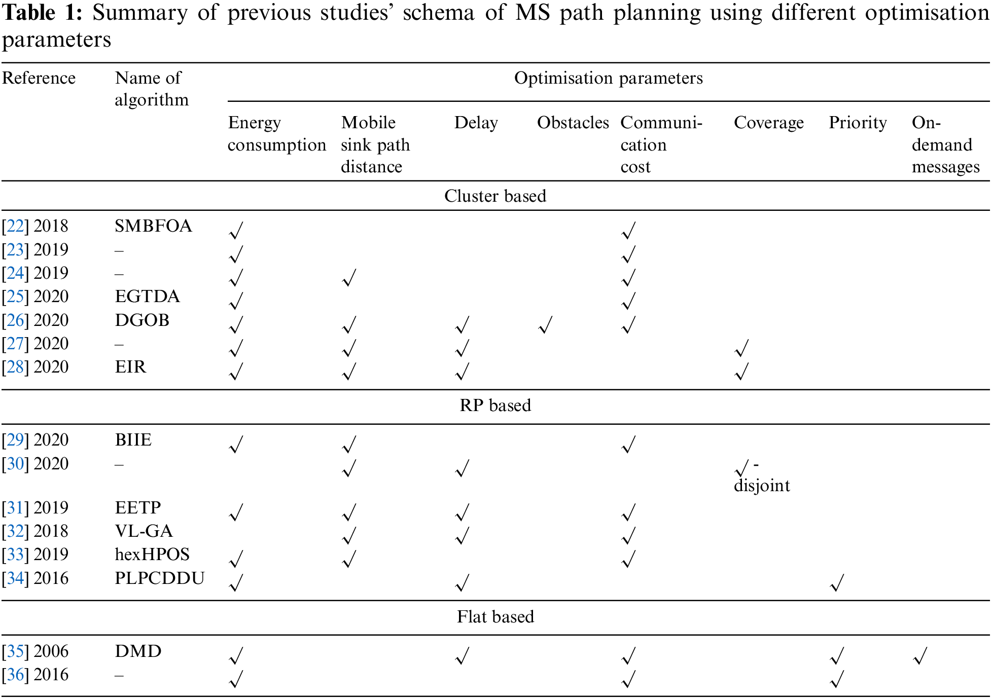
However, as Tab. 1 shows, researchers have not often recently examined optimisation parameters such as area priority and on-demand messages. Regarding the priority parameter, different uses of priority have been conducted, as mentioned in previous studies [34–36]. Each of these studies has different tasks utilising priority that positively affects network performance.
The other parameter, on demand, is considered essential when the monitoring field involves sudden urgent events, either frequently or rarely. These messages could cause a buffer overflow that exceeds the storage allocated for transmitted data. Thus, if urgent messages are not delivered immediately, the traffic data at some SNs could drop or overwrite. In one research [35] reviewed earlier, urgent messages were rare. When they occur, they are routed to the nearest neighbouring SNs that the MS frequently visits in a small monitoring field. However, if urgent messages occur frequently in some areas for monitoring or tracking important events, such as in a battlefield in a large area, the MS could visit these SNs after a period, causing delayed arrival of these data, which results in non-tolerance time or loss of packets because of buffer overflow. Therefore, prior researchers have assigned priority to the sensor data rate (message) or SNs in the rare edges of transmitting data to the MS, but the priority of an area that can include more than one SN with high data rates (urgent messages) in a large area has not been investigated.
Thus, the present study takes advantage of the priority parameter to utilise it differently from previous research to increase the performance of the MS for gathering data in a large monitoring field with sudden, frequent urgent messages. The MS moves first to those sub-areas with higher-priority frequent urgent messages to collect data while avoiding their rerouteing or loss.
For the on-demand parameter (where urgent messages occur), this research was aimed at minimising delays and maximising the data packet ratio. Thus, in addition to considering the priority for the sub-areas containing SNs with urgent messages, routeing urgent messages to the MS position is proposed. SNs with urgent messages should deliver their data immediately to the MS position. Their importance relative to that of the MS is different from that reported in previous studies [35]. Waiting for the MS to arrive leads to SNs losing data due to buffer overflow or delayed arrival at the application end users.
However, adding more parameters to MS path planning, such as priority and routeing urgent messages, can increase the efficiency of the MS in collecting sensor data. MS path planning algorithms can be improved to increase SN energy efficiency; minimise the time needed to collect data from SNs, especially when urgent messages occur; and maximise the data packet ratio. Thus, the EEPP-BAP is proposed to address these parameters and enhance the performance of the WSN with MS. The next section explains the framework of the proposed EEPP-BAP method in detail.
In this section, the proposed EEPP-BAP framework is explained in detail. The EEPP-BAP framework combines the functionality of collecting application-monitoring data from stationary SNs by using MS path planning and handling special cases of urgent messages occurring outside the scheduled or planned MS path. As explained earlier, energy efficiency is widely accepted as the main issue in WSNs because WSN operations depend heavily on the lifespan of SN batteries. Consequently, it is essential to develop an energy-efficient MS path planning scheme, especially for large-scale WSNs. Therefore, repositioning the sink at a regular time interval, considering the priority and distance of each sub-area can minimise energy consumption and delivery delay by avoiding the extensive routeing of real-time urgent messages and decreasing the failure rate. As the network structure is cluster based, which can prolong the network lifetime, the MS should collect data by moving along a predesigned path to reach each CH node in a regular round. Therefore, the proposed EEPP-BAP method consists of four procedures: partitioning the area into zones; clustering and CH selection; constructing the path plan of the MS; and establishing the routeing of urgent messages to the MS position, an additional procedure in case the MS is not at the SNs that contain urgent messages. Fig. 4 illustrates these procedures.

Figure 4: Procedure for the EEPP-BAP method
3.1 Area Partitioning and Priority Assigning
The EEPP-BAP framework first gives higher priority to the areas for which the monitoring data were generated than to the other areas (e.g., urgent messages appear frequently). Thus, the first procedure in EEPP-BAP is to partition the monitored area into zones and assign each zone priority. The priority could be assigned by the application user or automatically based on the calculated data generation rate. The zones could be equal or variable in size, depending on the size of the areas that are more exposed to high-data-rate messages. Furthermore, zones that are geographically separated are allowed to have the same priority. As a result, the priority assignment step assists in ranking the zones according to importance, which should be considered first by the MS for data collection.
The EEPP-BAP method equally divides a square monitoring field into zones for simplicity, as presented in Fig. 5A, using the following equation:

Figure 5: Simple example of the EEPP-BAP steps: (A) partitioning the area, (B) assigning the priority, (C) clustering the area, (D) MS path planning, and (E) routeing urgent messages to the MS position
Eq. (1) calculates the total monitoring field area, where n is the length of a side of the monitoring area.
To obtain the required number of zones, Eq. (2) is calculated, expressed as follows:
where
The division of the monitoring field into zones and assigning each zone a priority are followed by clustering and CH selection.
3.2 Clustering and CH Selection
In this procedure, the SNs in the monitored field are grouped into clusters to conserve energy and reduce routeing overhead. Similar to most routeing protocols in WSNs, as explained in Section 1, the resulting network structure will be hierarchical, with two levels of CH and CM. The clusters created are irrelevant to the defined zones. This means that one cluster could span two zones, or one zone could include more than one cluster.
In the first step, EEPP-BAP builds the neighbouring matrix that has the distance information parameter between SNs by using the Euclidean distance algorithm, expressed as follows:
where
However, the EEPP-BAP method clusters SNs based on the CH selected. After CH selection, as explained below, the neighbours of the CH are connected to comprise one cluster with single-hop communication.
CH Selection Using PSO
Proper CH selection contributes significantly to balancing and conserving energy, which enhances the WSN lifetime. In the EEPP-BAP method, three parameters are used to optimise the CH selection. These parameters are SN residual energy, the average distance between SNs, and the degree of SNs [37].
• Residual energy measures the energy of each SN in the cluster with respect to other nodes. This prevents those SNs with less energy from being selected as CH to balance and conserve energy among SNs. It is measured using the following equation:
where the number of members in the current cluster is represented as
• The second parameter, the average distance between SNs, is needed to further conserve energy and minimise delivery delays to the greatest possible extent. It is calculated using the following equation:
where again
• The last parameter is node degree, which represents the number of members covered by a CH. A sensor connected to more nodes reflects greater efficiency in receiving more packets [37]. This is calculated using the following equation:
Finally, the variable
Fig. 5C shows a simple example of clustering and CH selection based on three parameters using PSO.
PSO-based CH selection:
Based on the gathered information on SNs in each cluster, the PSO algorithm was implemented to select the most suitable CH based on SN residual energy, the average distance between SNs, and the degree of SNs. The proposed EEPP-BAP method is used to perform the PSO algorithm to select the CH owing to its many advantages. These advantages include swift convergence, application in dynamic situations, and simple computation [38–40]. The steps of PSO generally involve four processes: initialisation, computing, updating, and evaluation.
A) The initialisation step is for initialising the population of named particles
B) The computation step is performed using the fitness function, which represents the objectives of a certain problem. This function is performed for each particle as its input and then produces the output to evaluate the ‘goodness’ of these particles. In this step, the particles continue tracking with the personal best value (
C) The updating step is for
where
D)
Therefore, the updating values of
These four steps of PSO are designed to obtain the best solution by finding the best position for each particle evaluated using the fitness function. Thus, in the proposed EEPP-BAP method, each particle forms a candidate-completed solution that represents the optimal CH selection for each cluster evaluated using the fitness function. To formulate the fitness function, the EEPP-BAP method adapts the three parameters expressed in Eqs. (5)–(7). The fitness function obtains the maximum value of the combined three objectives, as expressed in the following equation:
where
Therefore, after performing the two procedures, the best MS visit is determined according to CH selection to plan the MS path with respect to the zone priorities. Thus, MS path planning considers more parameters to construct the MS path to increase the efficiency of the network, as explained in the next procedure.
3.3 MS Path Planning Using BSO
Constructing the MS path within a clustered WSN using the selected CHs is performed by selecting the CH positions to move the MS efficiently among them. For each cluster, the MS moves to each CH to collect the monitoring data that must reach the base station. In the proposed EEPP-BAP method, the zone priority and distance from the CH are the parameters considered when constructing the MS path. The priority assigned to the partitioned zones (Section 3.1) in the first procedure of the EEPP-BAP is used in MS path planning. The path starts from the CHs in the zones with the highest priority. This improves the performance of the network by prioritising CHs with more data that must be collected first. Moreover, when urgent messages occur, this prevents the rerouteing of urgent messages from higher-priority zones, as shown in Fig. 5D. Extensive routeing of these messages causes an energy imbalance in the network. In addition, if there are CHs located in zones with equal priorities, the MS will be assigned to move to the nearest CH to collect its data. This is where the second parameter, distance, is needed in MS path planning.
To ensure optimisation in MS path planning, the EEPP-BAP method applies the BSO algorithm to construct the MS path. The fitness function of the algorithm includes the two parameters of zone priority and distance, as explained in the following steps:
BSO-based MS path planning:
Based on the construction of the MS path plan, the BSO algorithm was implemented to select the most suitable path based on zone priority and distance. The proposed EEPP-BAP method performs the BSO algorithm to construct the path, as this method has been used in many applications [9]. BSO has four main operators: initialisation, clustering the solution, generating, and selection.
A) The initialisation operator is used to initialise the population of named individuals
B) Clustering the solution operator involves a convergence process. This operator groups the similar solutions
C) The generation operator produces new individuals by mutation. This operator utilises divergence to generate new individuals from the cluster centre with the best fitness function or from a non-cluster centre using one or more old individuals from one or more clusters. Thus, Gaussian mutation is used to generate new individuals expressed as follows:
where
D) The selection strategy decides which new individuals with better fitness function values to retain for the next iteration. This iteration continues until the condition that satisfies the value is met or the method is assumed to have converged. These BSO operators are aimed at obtaining the best solution by reducing the search space by clustering the ideas and generating new individuals from the old individuals with the best fitness function value, expressed as follows:
Thus, in the proposed EEPP-BAP method, each individual (idea) comprises candidate-completed solutions for MS path planning that have the same dimension D evaluated by the fitness function. To formulate the fitness function for MS path planning in this research, the proposed EEPP-BAP method combines two parameters: zone priority and the shorter distance between CHs and
Priority zones. The
Distance from
where
where
When the algorithm reaches a satisfied value that represents the optimal MS path or when the method assumes convergence, the process terminates. After the optimal selection of the MS, normal data collection starts and continues until a change in the network occurs; for example, the CH energy is lower than a certain threshold, or a zone priority changes.
During normal MS operations, there are special cases in which urgent messages must be delivered to the MS. These urgent messages should be delivered immediately; otherwise, they might get lost because of buffer overflow, causing a decline in the network throughput, a delay due to the retransmission of the same data packets, and a reduction in energy efficiency due to wastage of resources. Consequently, the network lifetime is reduced. An example of urgent messages is sudden contingency events in zones where the MS has either not yet or already visited. To alleviate this problem, establishing the routeing of urgent messages to the MS position is considered the next procedure of the proposed EEPP-BAP method.
3.4 Establishing the Routeing of Urgent Messages to the MS Position Using PSO
Some zones, especially those with higher priorities, tend to have urgent messages at any time. Thus, the MS visiting each CH one time per round is insufficient because of the urgent messages after or before MS visits. Thus, in the EEPP-BAP framework, a procedure for handling urgent messages was added in parallel with the normal MS path planning procedure. It is important to handle urgent messages separately by applying an efficient and optimised routeing algorithm as discussed in previous studies [35,40–42]. This is because ignoring urgent messages until the next MS round will negatively affect network performance and lifetime. This procedure is a special case that does not happen in each round of data collection.
Routeing urgent messages refers to a situation in which any SN with urgent messages transfers its data to the MS position. Urgent messages are routed by selecting SNs between the source and the MS, named RNs. Messages can be transmitted using single- or multi-hop communication. Moreover, an RN is an SN that can also be a CH or CM in the network. In the urgent message routeing procedure, two parameters are considered: the distance between SNs and MS and residual energy. Selecting the SNs with the shortest distances to the MS helps in the delivery of urgent messages with minimum delay. In addition, selecting the SNs with the highest residual energy leads to an energy consumption balance among SNs by preventing SNs with less energy from acting as RNs. Thus, the proposed EEPP-BAP method considers these two parameters to optimise the selection of RNs for routeing urgent messages to the MS position using the PSO algorithm.
However, urgent messages are routed to the MS position between CH to CH within communication range and between CH to MS through multi-hop communication. When there is no CH within communication range, then the neighbouring node (CM) is selected as the next RN. Moreover, the CH can transmit urgent messages directly through single-hop communication to the MS if the distance between them is shorter than the distance between the CH and other CHs. The selection between RNs is based on the shortest distance to the MS position and the SNs with the highest residual energy to formulate the fitness function in the next section. Fig. 5E shows a simple process of routeing urgent messages to the MS position using PSO.
PSO-based RN selection:
Based on routeing urgent messages to the MS, the PSO algorithm is implemented to select the most suitable RNs through multi-hop communication based on SN residual energy and the average distance between SNs with urgent messages relative to the MS position. The PSO steps were previously discussed in Section 3.2.
Thus, in the proposed EEPP-BAP method, each particle forms a candidate-completed solution that represents the optimal relay SNs, having the routeing path from the SNs with urgent messages to the MS position evaluated by the fitness function.
To formulate the fitness function of the selection relay SNs, the proposed EEPP-BAP method is performed to select the next hop of relay SNs based on the minimum path distance and highest residual energy, as in a prior study [37]. However, the proposed EEPP-BAP method reformulates the fitness function in relation to the MS position and considers the neighbouring SNs beside the CHs, expressed as follows:
1. Distance from the SN to the MS (dis): The SN with urgent messages, represented as
where
where
where
Therefore, to compute the minimum distance to route urgent messages between the current SNs and the MS, the following equation is applied:
2. Residual energy: The energy of the SNs is measured for each SN that is a candidate RN. This prevents the SN with less energy from being selected as a RN. Thus, this parameter is expressed as follows:
First, residual energy is computed per round as follows [42]:
where
where
Therefore, by combining these two objectives, the fitness function is formulated to obtain the minimum value expressed as follows:
where
After explaining the four procedures of the EEPP-BAP method, we present in the next section the experiments using the proposed method in comparison with other studies using simulation.
This section discusses the simulation environment for the EEPP-BAP method. Moreover, it illustrates the amount of data generated by SNs using the Poisson distribution method and the energy consumption and packet reception rate (PRR) of both models, which are used for simulation purposes in WSNs.
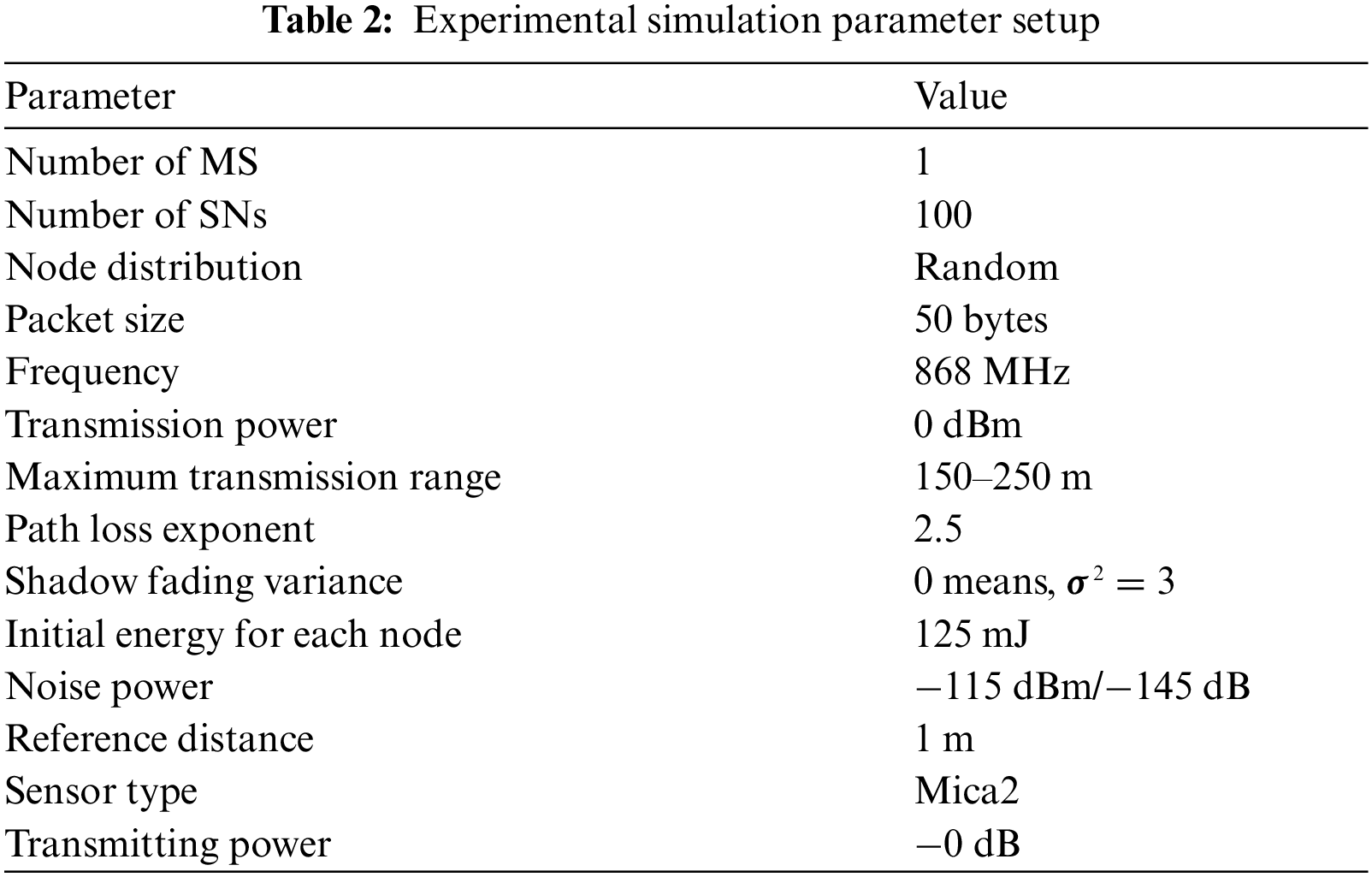
In this research, the simulation environment consisted of 100 stationary SNs deployed at random on a field of 1000 × 1000 m (large area) and one MS. All the later simulation experiments were performed for homogeneous SNs with the same capability and specification on a custom, and their locations were awarded using a MATLAB simulator. Fig. 6 provides a simplified illustration of the EEPP-BAP procedure starting from the random deployment of SNs and sink node/MS placement up to MS path planning.

Figure 6: Simple illustration of the main procedures of the proposed EEPP-BAP method. (A) SN distribution and MS placement. (B) Area partitioning and zone assigning. (C) Area clustering and CH selection. (D) MS path planning
4.2 Generating Data in the Network
Data traffic on the SNs is generated based on the Poisson process of intensity λ packets per second [43]. The Poisson process represents a model that describes a random event occurring by finding the number of probable events over a certain time by using the Poisson distribution expressed as
where λ is the rate parameter representing the event/time × time period. The λ value expresses the data traffic in the network, divided into urgent and non-urgent. In later experiments, the value of λ ranged from 3 to 11.
In addition, the harsh wireless channel model was chosen, including shadowing and fading effects and noise. The simulation parameters are outlined in Tab. 2.
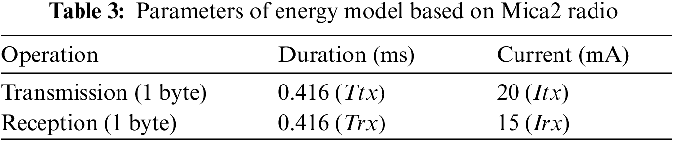
The energy consumption model utilised in the EEPP-BAP simulation and used for the evaluation of the performance metrics explained in Section 5 is described here. It refers to the summation of the amount of energy consumed to transmit or receive the data packet by SNs, expressed as follows:
where
The PRR model is utilised in EEPP-BAP to measure the loss or quality of the link in the WSN, which means that the data packet arrives at the correct MS. It is used in the next section to evaluate performance metrics. This has been adopted from the PRR metric used in a prior study [44], which was built using wireless channel statistics, expressed as
where
where
where
In this section, we describe the various experiments we conducted to achieve our objectives and evaluate the effectiveness of the proposed solution. These simulation experiments consist of six experiments as shown in Fig. 7. The first three experiments study the variation of network lifetime, packet delivery rate, and end-to-end delay with respect to the average traffic load. The average traffic rate changes from 3 to 11. In addition, through the last three experiments, the total energy consumption, average residual energy of sensor nodes, and the energy imbalance factor have been calculated during the running time. The performance metric parameters are presented first, followed by the simulation results.

Figure 7: Performance metrics for testing the simulations
5.1 Performance Metric Parameters
The performance of our proposed EEPP-BAP method was evaluated using the following metrics:
• Network Lifetime [45]: This refers to the time until the first SN runs out of battery after starting network operation. To calculate the lifetime of each SN, the following equation is applied:
In the equation, if any
• Packet delivery ratio (PDR) [46]: This defines the ratio of the data packets sent to the MS by SNs, without packet loss. This is determined using the PRR model, considering the entire number of data packets to measure the reliability of the network, and is expressed as
• Average end-to-end delay (AveDelay) [47]: This represents the average time for N, which represents the entire SN spent to route or transmit a data packet from the source to the target destination. This includes propagation, transmission, transmission and reception current delay, and retransmission. The processing delay can be ignored as a result of the fast processing speed, which is expressed as:
• Energy consumption (EC) [48]: This represents the whole energy in the network that N consumes to transfer and receive the data packet. Therefore, EC is the total summation of the energy consumed by each SN
• Average residual energy (
where the total number of SNs is represented as N and the energy of each SN is represented as
• Energy Imbalance Factor (EIF) [50]: This indicates the standard deviation of the residual energy of all SNs in the network. It measures the efficiency of the energy balance during running time in the network, expressed as
Performance was compared to verify the feasibility and effectiveness of the proposed method in terms of network lifetime, energy consumption, average end-to-end delay, and average residual energy with the algorithms presented in previous studies [22,25]. To compare the performance of the parameters used in the proposed EEPP-BAP method with the other parameters used [22,25], in all later experiments, all algorithms were considered to have the same environment, clustering, and delivery of urgent messages to the MS using the routeing technique described in a previous study [37]. The differences lie in the selection of parameters for the movement of the MS.
5.2.1 Network Lifetime Evaluation
In this experiment, the performance evaluation of the proposed method, EEPP-BAP, was compared with two previously published studies [22,25] in terms of network lifetime. Based on the average traffic rate λ, the simulation experiment studies showed that the network lifetime varies when the first node dies. To test this variation, a simulation experiment was started by varying the average traffic rate λ from 3 to 11. Fig. 8 shows the variation in the network lifetime under different average values of the traffic rate λ. From Fig. 8, it can be clearly seen that the network lifetime decreases as the value of λ increases. As the network traffic increases with increments of λ, the relay loads of the node increase, leading to more energy consumption. Moreover, the higher the traffic rate, the more incoming data packets at each SN, which leads to a smaller buffer space, which in turn leads to a higher waste of energy due to the retransmission of lost packets resulting from buffer overflow. Consequently, the network lifetime decreases. However, the figure illustrates obviously how the proposed method remarkably enhanced the network lifetime while increasing the average traffic rate in comparison with the other traffic rates in the network. The proposed method effectively conserves the network energy consumption, which can be attributed to two reasons: The first reason is that the proposed path plan considers the zone priority, which can provide a significant improvement in the network lifetime, as it conserves energy consumption. This can be justified as follows: the zones with higher priority than others in gathering data are expected to have urgent messages that should be evaluated first for the MS to behave and respond quickly. Thus, considering such areas avoids urgent message routeing to the MS and positively affects the network lifetime by consuming less energy. Second, the proposed algorithm utilises the distance to the MS to reduce energy consumption.

Figure 8: Comparison of network lifetime and average traffic rate for a homogeneous network
In the case of the algorithm from Hamidouche et al. [22], the MS visits the CH at each cluster based on the nearest CH, according to its current position, which is based on distance. In the algorithm from Bencan et al. [25], as a new location for the sink node, a cluster with higher residual energy and a closer distance from other clusters is chosen. Nevertheless, they suffer from being unaware of information about the zone/area priority, resulting in energy wastage due to the routeing of urgent messages to the MS position, which exposes the SNs to consume more energy in multi-hop communication and thus negatively affects network lifetime.
Tab. 4 shows the percentage improvement in the network lifetime with the proposed method compared with that achieved in the previous works [22,25]. For example, at a λ value of 11 packets per second, the proposed method achieved a network lifetime of approximately 6400 s, whereas the lifetimes achieved in the previous works [22,25] were 2400 s and 2100 s, respectively. This means that the proposed method can achieve approximately 166.6% and 204.7% improvements in network lifetime compared with the results of the works of Hamidouche et al. [22] and Bencan et al. [25], respectively.

When traffic load increases, more packets are pushed into the network, which can cause congestion and packets to be dropped.
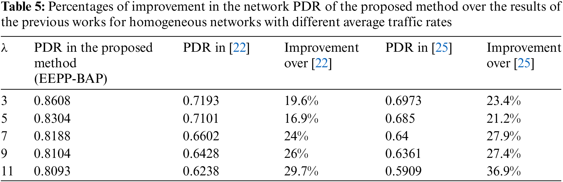
In this experiment, we compared the performance of the proposed method with those of two previous studies using the PDR metric [22,25] for homogeneous networks. With this simulation experiment, we examined how network PDR varies with the average traffic rate λ for homogeneous networks. This experiment started by increasing the average traffic rate λ from 3 to 11. Fig. 9 shows the variation of the network PDR with the average traffic rate λ. In general, with an increase in the average traffic rate, the network traffic load increases. This is due to increases in the number of packets pushed into the network as traffic load increases; thus, congestion and dropped packets can occur in the network. However, the figure shows that the network throughput of the proposed method slightly decreased as the average traffic rate increased. Meanwhile, the proposed method obtained the highest PDR compared with the other PDRs even while increasing the average traffic rate in the network because the proposed method attempted to avoid urgent message routeing to the MS by considering the zone/area priority. During multi-hop wireless communication, data packets are lost as a result of the dynamic nature of wireless communication links and unstable channel conditions. Thus, avoidance of urgent message routeing enhances the network PDR, as it prevents packets from going to possible unreliable paths. On the contrary, the previous works [22,25] did not consider zone/area priority, where loss of packets reduced the network throughput as a result.

Figure 9: Comparison of PDR and traffic rate for homogeneous networks
Tab. 5 shows the percentages of improvement in the network PDR of the proposed method over the results of the previous works with different data rates. For example, at λ of 7 packets per second, the proposed method has a network PDR of approximately 0.8188. Meanwhile, the PDR value obtained in the first previous work [22] was 0.6602, while it was 0.6400 in the second previous work [25]. This means that the proposed method can achieve approximately 24% and 27.9% improvements in network PDR compared with the results achieved in the previous works [22,25], respectively.
5.2.3 Evaluation of Average End-to-End Delay
This experiment compares the performance of the proposed method with that of previous studies in terms of end-to-end delays in homogeneous networks.
In this experiment, we compared the performance of the proposed method with those of the methods reported in previous studies [22,25] in terms of end-to-end delay in homogenous networks. The average traffic rate λ is used to study the variation in average end-to-end delay in this simulation experiment. The experiment starts by increasing the average traffic rate λ in a network. Fig. 10 shows the variation of the average end-to-end delay with the average traffic rate. The simulation results clearly show that the end-to-end delay increases with the average traffic rate. When traffic rates are high, the number of incoming packets from a node increases, thereby reducing the buffer space and resulting in a higher probability of buffer overflows. In other words, end-to-end delay increases as a result of queuing delay and delay due to the retransmission of lost packets.

Figure 10: Average end-to-end delay according to traffic rate for homogeneous networks
However, based on the comparison of the different methods, the proposed method obtained the lowest end-to-end delay. This can be justified as follows: the proposed method avoids the routeing of urgent messages as much as possible, which in turn reduces propagation delays. Moreover, as the proposed model prevents packets from going to possible unreliable paths, the delay due to the retransmission of the lost packets is decreased. In the case of the previous works [22,25], the urgent messages move to the MS on long paths due to multi-hop transmissions, thus increasing the packet propagation delay. In addition, the transmission over the lossy wireless links increases the delay due to the retransmission of the lost packets. Tab. 6 shows the percentages of the improvement in average end-to-end delay with the proposed method over the results of the previous works [22,25] with different data rates. For example, at a λ value of 7 packets per second, the proposed method achieved an end-to-end delay of approximately 0.3316 s. On the other hand, the end-to-end delays achieved in the previous works were 0.3571 and 0.3533 s, respectively. This means that the proposed method can achieve approximately 7.1% and 6.7% improvements in the average end-to-end delay when compared with the results of the previous works.

5.2.4 Energy Consumption Evaluation
The proposed EEPP-BAP method was compared with the previous works [22,25] in this experiment, which was performed to evaluate energy consumption. During operation of the network, the energy consumption was calculated to observe the network energy efficiency, which adapted the energy consumption model described in Section 4.1.2. The average traffic rate λ is fixed at 7 packets per second. As shown in Fig. 11, the energy consumption varied over time during the simulation. The simulation results presented in the figure verify that energy consumption increases with increases in running time. Thus, as the proposed method achieved a longer lifetime than the methods described in the previous works [22,25], the proposed method used less energy during the network process, as illustrated in Fig. 11.

Figure 11: Energy consumption according to simulation time for homogeneous networks
5.2.5 Average Residual Energy Evaluation
In this experiment, the performance of the proposed method was evaluated in terms of energy balance compared with the presented algorithms in [22] and [25]. The average residual energy was calculated during the running time to determine the balance efficiency of the network. The average traffic rate λ is fixed to 7 packets per second. Fig. 12 presents the variation in the average residual energy over the simulation time. The figure clearly shows that the average residual energy decreases with a longer running time. Indeed, in random topologies, some areas are highly dense, whereas others are less dense. As these areas do not necessarily overlap, an imbalance in the distribution of sensors is subsequently enforced. Undoubtedly, the average residual energy across the network is negatively affected. It is for this reason that the average residual energy decreases with increased running time. However, the average residual energy of the proposed method can balance energy consumption efficiently better than the methods used in the previous studies [22,25]. This is due to the preservation of node energy per round as a result of the minimal energy consumption due to the energy-efficient path planning algorithm.

Figure 12: Average residual energy according to simulation time for homogeneous networks
In this experiment, the performance of the proposed method was evaluated in terms of EIF compared with the presented algorithms in the previous studies [22,25]. The network balance efficiency was calculated using the EIF metric during the running time. The average traffic rate λ is fixed to 7 packets per second. The EIF variation over the simulation time is shown in Fig. 13, which is clearly augmented with a longer running time. This is due to the different average amounts of residual energy of the areas with different densities of SNs in the network caused by the random distribution of the SNs. However, the proposed method achieved a lower EIF value during network execution compared with the previous methods [22,25]. This illustrates that the energy use in the proposed method approaches the average energy of the entire network, which attains energy balance. Therefore, the proposed method can balance energy use more effectively than the previously described methods [22,25] because the proposed method attempts to avoid extensive routeing and minimise hop count by considering priority relative to using the MS. Thus, in the proposed model, the energy consumption in SNs preserved energy remarkably. Although all the methods used the residual energy parameters at CH and RN selection for routeing urgent messages, in the study by Bencan et al. [25], the stability of the curve for energy consumption due to the method used primarily depended on the energy balance of the MS movement. From the results of these experiments, we can conclude that the proposed method improved the data collection process in WSNs.

Figure 13: EIF according to simulation time in the network
In this study, the EEPP-BAP framework is proposed to further improve the overall efficiency of WSNs and application monitoring data collection. The EEPP-BAP utilises two additional parameters for MS deployment in WSNs. One parameter defines zone priority, and the other uses on-demand routeing requests. The four processes in the framework were defined, and their operations were explained. Moreover, the PSO and BSO algorithms were adapted to solve optimisation issues in the WSNs. They were used in the CH selection, constructing the MS path plan and routeing urgent messages to the MS position. These two added parameters significantly impacted network performance. This was demonstrated through simulations and comparisons with other approaches that used different parameters to construct MS path plans based on distance [22] and on distance and energy [25]. The comparisons showed that the performance of the proposed method was better in terms of maximising energy efficiency up to 206.6% on average, minimising data packet loss up to 36.9% on average, and minimising urgent message delivery time up to 7.1% on average. In future research, with the delay-bound parameter that refers to a certain deadline for message arrival at the sink, and multiple MS can be distributed differently on a large-scale monitoring field. Moreover, future research can consider the sub-areas with greater priority in the MS path using the zigzag technique to further minimise the routeing of urgent messages.
Acknowledgement: We thank King Abdul-Aziz University (KAU) for giving us the opportunity to conduct this research.
Funding Statement: This research was supported and funded by the KAU Scientific Endowment, King Abdul-Aziz University, Jeddah, Saudi Arabia.
Conflicts of Interest: The authors declare that they have no conflicts of interest to report regarding the present study.
1. S. Gupta and P. Sinha, “Overview of wireless sensor network: A survey,” International Journal of Advanced Research in Computer and Communication Engineering, vol. 3, no. 1, pp. 5201–5207, 2014. [Google Scholar]
2. A. Gupta, H. Gupta, P. Kumari, R. Mishra, S. Saraswat et al., “A real-time precision agriculture monitoring system using mobile sink in WSNs,” in IEEE Int. Sym. on Advanced Networks and Telecommunication Systems (ANTS), Indore, India, pp. 1–5, 2018. [Google Scholar]
3. C. Xu, Z. Xiong, G. Zhao, S. Yu and S. Member, “An energy-efficient region source routing protocol for lifetime maximization in WSN,” IEEE Access, vol. 7, pp. 135277–135289, 2019. [Google Scholar]
4. B. Al-kaseem, Z. Taha and S. Abdulmajeed, “Optimized energy—efficient path planning strategy in WSN with multiple mobile sinks,” IEEE Access, vol. 9, pp. 82833–82847, 2021. [Google Scholar]
5. M. Krishnan, Y. Jung and S. Yun, “An improved clustering with particle meta optimization-based mobile sink for wireless sensor networks,” in Conf. on Trends in Electronics and Informatics (ICOEI), Tirunelveli, India, pp. 1024–1028, 2018. [Google Scholar]
6. W. Heinzelman, A. Chandrakasan and H. Balakrishnan, “Energy-efficient communication protocol for wireless microsensor networks,” in IEEE Hawaii Int. Conf. on System Science, Maui, HI, USA, pp. 1–10, 2000. [Google Scholar]
7. S. Nasr and M. Quwaider, “LEACH protocol enhancement for increasing WSN lifetime,” in Int. Conf. on Information and Communication Systems (ICICS), Irbid, Jordan, pp. 102–107, 2020. [Google Scholar]
8. A. Forster, “Multi-hop communications,” in Introduction to Wireless Sensor Networks, 1st ed., Hopkin, New Jersey, USA: John Wiley & Sons, Chapter No. 5, Section No. 5.2.2, 2016. [Google Scholar]
9. E. Tuba, I. Strumberger, D. Zivkovic, N. Bacanin and M. Tuba, “Mobile robot path planning by improved brain storm optimization algorithm,” in IEEE Congress on Evolutionary Computation (CEC), Brazil: Rio de Janeiro, pp. 1–8, 2018. [Google Scholar]
10. R. Hamidouche, Z. Aliouat, A. Gueroui, A. Ari and L. Louail, “Classical and bio-inspired mobility in sensor networks for IoT applications,” Journal of Network and Computer Applications, vol. 121, no. 1, pp. 70–88, 2018. [Google Scholar]
11. A. Waheed Khan, A. Abdullah, M. Anisi and J. Iqbal Bangash, “A comprehensive study of data collection schemes using mobile sinks in wireless sensor networks,” Sensors, vol. 14, no. 2, pp. 2510–2548, 2014. [Google Scholar]
12. R. Vera-amaro, M. Angeles and A. Luviano-Juarez, “Design and analysis of wireless sensor networks for animal tracking in large monitoring polar regions using phase-type distributions and single sensor model,” IEEE Access, vol. 7, pp. 45911–45929, 2019. [Google Scholar]
13. L. Zhang and C. Wan, “Dynamic path planning design for mobile sink with burst traffic in a region of WSN,” Wireless Communications and Mobile Computing, vol. 2019, no. 1, pp. 1–8, 2019. [Google Scholar]
14. S. Mottaghi and M. Zahabi, “Optimizing LEACH clustering algorithm with mobile sink and rendezvous nodes,” AEU - International Journal of Electronics and Communications, vol. 69, no. 2, pp. 507–514, 2015. [Google Scholar]
15. S. Singh and P. Kumar, “A comprehensive survey on trajectory schemes for data collection using mobile elements in WSNs,” Journal of Ambient Intelligence and Humanized Computing, vol. 11, no. 1, pp. 291–312, 2020. [Google Scholar]
16. Y. Hu, X. Wu, F. Wang and H. Han, “A particle swarm algorithm based routing recovery method for mobile sink wireless sensor networks,” in Chinese Control and Decision Conf. (CCDC), Changsha, China, pp. 887–892, 2014. [Google Scholar]
17. S. Sackey, J. Ansere, J. Anajemba, M. Kamal and C. Iwendi, “Energy efficient clustering based routing technique in WSN using brain storm optimization,” in IEEE Int. Conf. on Emerging Technologies (ICET), Peshawar, Pakistan, pp. 1–6, 2019. [Google Scholar]
18. R. Ramadan, “Fuzzy brain storming optimization algorithm,” International Journal of Intelligent Engineering Informatics, vol. 5, no. 1, pp. 67–79, 2017. [Google Scholar]
19. M. Ab Wahab, S. Nefti-Meziani and A. Atyabi, “A comprehensive review of swarm optimization algorithms,” PLoS ONE, vol. 10, no. 5, pp. 1–36, 2015. [Google Scholar]
20. K. Stephen and V. Mathivanan, “An energy aware secure wireless network using particle swarm optimization,” in IEEE Int. Conf.: Promoting Entrepreneurship and Technological Skills: National Needs, Global Trends (MIC), Muscat, Oman, pp. 1–6, 2018. [Google Scholar]
21. S. Cheng, Q. Qin, J. Chen and Y. Shi, “Brain storm optimization algorithm: A review,” Artificial Intelligence Review, vol. 46, no. 4, pp. 445–458, 2016. [Google Scholar]
22. R. Hamidouche, M. Khentout, Z. Aliouat, A. Gueroui and A. Abba Ari, “Sink mobility based on bacterial foraging optimization algorithm,” in Int. Conf. on Computational Intelligence and Its Applications, Oran, Algeria, vol.522, pp. 352–362, 2018. [Google Scholar]
23. F. Chao, Z. He, A. Pang, H. Zhou, J. Ge et al., “Path optimization of mobile sink node in wireless sensor network water monitoring system,” Complexity, vol. 2019, no. 10, pp. 1–10, 2019. [Google Scholar]
24. M. Krishnan, S. Yun and Y. Jung, “Dynamic clustering approach with ACO-based mobile sink for data collection in WSNs,” Wireless Networks, vol. 25, no. 8, pp. 4859–4871, 2019. [Google Scholar]
25. G. Bencan, D. Panpan, C. Peng and R. Dong, “Evolutionary game-based trajectory design algorithm for mobile sink in wireless sensor networks,” International Journal of Distributed Sensor Networks, vol. 16, no. 3, pp. 155014772091100, 2020. [Google Scholar]
26. S. Najjar-Ghabel, L. Farzinvash and S. Razavi, “Mobile sink-based data gathering in wireless sensor networks with obstacles using artificial intelligence algorithms,” Ad Hoc Networks, vol. 106, pp. 1–12, 2020. [Google Scholar]
27. N. Gharaei, K. Abu Bakar, S. Z. M. Hashim and A. H.Pourasl, “Inter- and intra-cluster movement of mobile sink algorithms for cluster-based networks to enhance the network lifetime,” Ad Hoc Networks, vol. 85, no. 4, pp. 60–70, 2019. [Google Scholar]
28. N. Gharaei, K. Abu Bakar, S. Z. M. Hashim and A. H.Pourasl, “Energy-efficient intra-cluster routing algorithm to enhance the coverage time of wireless sensor networks,” IEEE Sensors Journal, vol. 19, no. 12, pp. 4501–4508, 2019. [Google Scholar]
29. X. Fu and X. He, “Energy-balanced data collection with path-constrained mobile sink in wireless sensor networks,” AEU International Journal of Electronics and Communications, vol. 127, no. 2, pp. 1–11, 2020. [Google Scholar]
30. R. Anwit, A. Tomar and P. Jana, “Tour planning for multiple mobile sinks in wireless sensor networks: A shark smell optimization approach,” Applied Soft Computing Journal, vol. 97, no. 1, pp. 1–16, 2020. [Google Scholar]
31. X. He, X. Fu and Y. Yang, “Energy-efficient trajectory planning algorithm based on multi-objective PSO for the mobile sink in wireless sensor networks,” IEEE Access, vol. 7, pp. 176204–176217, 2019. [Google Scholar]
32. R. Anwit and K. Prasanta, “A variable length genetic algorithm approach to optimize data collection using mobile sink in wireless sensor networks,” in IEEE Int. Conf. on Signal Processing and Integrated Networks (SPIN), Noida, India, pp. 73–77, 2018. [Google Scholar]
33. S. Sun, J. Zhao, X. Feng, J. Zhang and J. Luo, “Mobile multi-sink nodes path planning algorithm concerned with energy balance in wireless sensor networks,” IEEE Access, vol. 7, pp. 96942–96952, 2019. [Google Scholar]
34. S. Juvvalapalem and K. Rao, “Sencar scheduling algorithm based on packet lifetime in WSN’s,” Indian Journal of Science and Technology, vol. 9, no. 17, pp. 1–5, 2016. [Google Scholar]
35. Y. Gu, D. Bozda and E. Ekici, “Mobile element based differentiated message delivery in wireless sensor networks,” in IEEE Int. Symp. on a World of Wireless, Mobile and Multimedia Networks (WoWMoM'06), Buffalo-Niagara Falls, NY, USA, pp. 1–10, 2006. [Google Scholar]
36. S. Say, H. Inata, J. Liu and S. Shimamoto, “Priority-based data gathering framework in UAV-assisted wireless sensor networks,” IEEE Sensors Journal, vol. 16, no. 14, pp. 5785–5794, 2016. [Google Scholar]
37. C. Vimalarani, R. Subramanian and S. Sivanandam, “An enhanced PSO-based clustering energy optimization algorithm for wireless sensor network,” Scientific World Journal, vol. 2016, no. 1, pp. 1–11, 2016. [Google Scholar]
38. H. Phan, K. Ellis and J. Barca, “A survey of dynamic parameter setting methods for nature-inspired swarm intelligence algorithms,” Neural Computing and Applications, vol. 32, no. 2, pp. 567–588, 2020. [Google Scholar]
39. A. Chakraborty and A. Kar, “Swarm intelligence: A review of algorithms,” Nature-Inspired Computing and Optimization. Modeling and Optimization in Science and Technologies, vol. 10, pp. 475–494, 2017. [Google Scholar]
40. P. Rao, P. Jana and H. Banka, “A particle swarm optimization based energy efficient cluster head selection algorithm for wireless sensor networks,” Wireless Networks, vol. 23, no. 7, pp. 2005–2020, 2020. [Google Scholar]
41. Z. Al Aghbari, A. Khedr, W. Osamy, I. Arif and D. Agrawal, “Routing in wireless sensor networks using optimization techniques: A survey,” Wireless Personal Communications, vol. 111, no. 4, pp. 2407–2434, 2020. [Google Scholar]
42. T. Tukisi, T. Mathaba and M. Odhiambo, “Multi-hop PSO based routing protocol for wireless sensor networks with energy harvesting,” in IEEE Conf. on Information Communications Technology and Society (ICTAS), Durban, South Africa, pp. 1–6, 2019. [Google Scholar]
43. Y. Li, C. Chen, Y. Song, Z. Wang and Y. Sun, “Enhancing real-time delivery in wireless sensor networks with two-hop information,” IEEE Transactions on Industrial Informatics, vol. 5, no. 2, pp. 113–122, 2009. [Google Scholar]
44. F. El-fouly, “Real-time energy-efficient reliable traffic aware routing for industrial wireless sensor networks,” IEEE Access, vol. 8, pp. 58130–58145, 2020. [Google Scholar]
45. N. Gharaei, S. J. Malebary, K. Abu Bakar, S. Z. Mohd Hashim, S. Ashfaq Butt et al., “Energy-efficient mobile-sink sojourn location optimization scheme for consumer home networks,” IEEE Access, vol. 7, pp. 112079–112086, 2019. [Google Scholar]
46. M. V. Babu and J. A. Alzubi, “An improved IDAF-FIT clustering based ASLPP-RR routing with secure data aggregation in wireless sensor network,” Mobile Networks and Applications, vol. 26, no. 3, pp. 1059–1067, 2021. [Google Scholar]
47. D. R. Edla, M. C. Kongara and R. Cheruku, “A PSO based routing with novel fitness function for improving lifetime of WSNs,” Wireless Personal Communications, vol. 104, no. 1, pp. 73–89, 2019. [Google Scholar]
48. S. Mottaghi and M. Zahabi, “Optimizing LEACH clustering algorithm with mobile sink and rendezvous nodes,” AEU International Journal of Electronics and Communications, vol. 69, no. 2, pp. 507–514, 2015. [Google Scholar]
49. B. Sahoo, T. Amgoth and H. Pandey, “Particle swarm optimization based energy efficient clustering and sink mobility in heterogeneous wireless sensor network,” Ad Hoc Networks, vol. 106, no. 4, pp. 1–21, 2020. [Google Scholar]
50. N. Kumar, V. Kumar, T. Ali and M. Ayaz, “Prolong network lifetime in the wireless sensor networks: An improved approach,” Arabian Journal for Science and Engineering, vol. 46, no. 4, pp. 3631–3651, 2021. [Google Scholar]
 | This work is licensed under a Creative Commons Attribution 4.0 International License, which permits unrestricted use, distribution, and reproduction in any medium, provided the original work is properly cited. |