Computers, Materials & Continua DOI:10.32604/cmc.2022.026246
Article

A Hybrid Neural Network-based Approach for Forecasting Water Demand

Al-Batool Al-Ghamdi1,*, Souad Kamel2 and Mashael Khayyat3

1Department of Computer Science and Artificial Intelligence, College of Computer Sciences and Engineering, University of Jeddah, Jeddah 21959, Saudi Arabia
2Department of Computer and Network Engineering, College of Computer Sciences and Engineering, University of Jeddah, Jeddah 21959, Saudi Arabia
3Department of Information Systems and Technology, College of Computer Sciences and Engineering, University of Jeddah, Jeddah 21959, Saudi Arabia
*Corresponding Author: Al-Batool Al-Ghamdi. Email: aalghamdi2633.stu@uj.edu.sa
Received: 20 December 2021; Accepted: 02 March 2022

Abstract: Water is a vital resource. It supports a multitude of industries, civilizations, and agriculture. However, climatic conditions impact water availability, particularly in desert areas where the temperature is high, and rain is scarce. Therefore, it is crucial to forecast water demand to provide it to sectors either on regular or emergency days. The study aims to develop an accurate model to forecast daily water demand under the impact of climatic conditions. This forecasting is known as a multivariate time series because it uses both the historical data of water demand and climatic conditions to forecast the future. Focusing on the collected data of Jeddah city, Saudi Arabia in the period between 2004 and 2018, we develop a hybrid approach that uses Artificial Neural Networks (ANN) for forecasting and Particle Swarm Optimization algorithm (PSO) for tuning ANNs’ hyperparameters. Based on the Root Mean Square Error (RMSE) metric, results show that the (PSO-ANN) is an accurate model for multivariate time series forecasting. Also, the first day is the most difficult day for prediction (highest error rate), while the second day is the easiest to predict (lowest error rate). Finally, correlation analysis shows that the dew point is the most climatic factor affecting water demand.

Keywords: Water demand; forecasting; artificial neural network; multivariate time series; climatic conditions; particle swarm optimization; hybrid algorithm

1  Introduction

Water is a precious resource for sustaining life on our planet. Currently, countries suffer from challenges in the availability of freshwater, as its availability may reach 44% of the global land area by the end of the century [1]. Water scarcity due to climate change caused pressure on governments to supply water to urban, industrial, and agricultural sectors. Studies have indicated that climate change will constitute a major limitation on urban water demand and will increase by 80% in 2050 [2]. The Food and Agriculture Organization of the United Nations (FAO) indicated that an increase in evaporation and a decrease in soil moisture can affect freshwater availability especially in arid regions [1]. Therefore, many researchers have focused on studying the impact of climate change [3–5].

The Kingdom of Saudi Arabia is the largest country in the Arabian Peninsula. It is located in the continent of Asia. It has a warm and dry desert climate with high temperatures above 50 degrees and an average rainfall of 114 ml per year [6]. Also, it suffers from a lack of water resources such as rivers and lakes. Since the United Nations classified Saudi Arabia as a country suffering from water scarcity, providing water to various sectors, as the demand increased by 70% from 2007 to 2018, constitutes a major challenge. So, to supply water, the government resorted to desalinating sea water. In 1970s, the first seawater desalination plant was established in Al-Jubail [6]. Now, it reaches 32 stations distributed on the eastern and western coasts of the century. Therefore, the Saline Water Conversion Corporation was classified as the largest corporation in the world for the production of desalinated water [7]. However, water desalination has negative effects on the environment, such as the emission of harmful gases into the air, as well as the consumption of 25% of fuel, which has an economic impact on the country [8]. Therefore, there is a need to accurately predict the amount of water demand under the arid climatic conditions in order to help the government to supply water to all sectors either in normal or emergency situations and to preserve the environment as well as the economy.

Forecasting can be classified into two types. The former is the short-term type. Its range is from one day to two weeks. The latter is the long-term type. Its range is longer than one year [9]. Also, forecasting can be classified either into univariate or multivariate. Univariate time-series forecasting is predicting the future based on one variable. While multivariate one depends on more than one variable to predict future values. Techniques used for forecasting can be divided into two classes: traditional techniques such as Autoregressive Integrated Moving Average (ARIMA), ineffective when dealing with large data or predicting multivariate time series [10], and Machine Learning (ML) techniques such as ANN, used for prediction, classification, recognition…etc. [11]. ANN is one of the most widely used techniques for forecasting because of its fault tolerance and its ability to deal with non-linear and complex data. Besides, ANN can be generalized after completing their training [12,13].

Seeking performance enhancement, many studies combined neural networks with other algorithms in the pre-processing phase or in the post-processing one, or for hyperparameters tuning [14–18]. Hyperparameter tuning is the process of enhancing a model’s performance to avoid overfitting and excessive variation [19]. It poses a great challenge to researchers and developers. Tuning them manually through Trial and Error, depends on the researcher’s experience. Wrong parameter tuning can cause a model inaccuracy. In fact, the parameter adjustment fluctuates the accuracy of the classification from 32.2% to 92.6% [20]. Instead of using Trial and Error, many techniques were used such as Grid search and PSO. In Grid search, researchers specify the minimum and maximum ranges, and the algorithm searches all possible combinations. But this consumes a long-time to find the optimal hyperparameters [21]. PSO which is a nature-inspired algorithm constitutes a good alternative. It is widely used to find the optimal hyperparameters since it is fast, easy to implement and can converge to a global optimum [22]. Haider et al. [23] presented an open-source package to select the optimal parameters using a PSO, named as “Package for parameters Selection using Particle Swarm Optimization (PSPSO).” This package selects the optimal number of neurons in hidden layers. It also specifies the learning rate, the optimal optimizer used to update weights, and the activation function in hidden and output layers. It supports four models. One of these models is Multilayer Perception (MLP), which is the most popular type of ANN used for forecasting [9]. However, one limitation of this package is that it is not dedicated to time series forecasting. Also, it does not support cross-validation for evaluating the prediction. Finally, it is built to be used only for classification and regression.

The above problems prompted us to improve the performance of ANN and select the optimal hyperparameters to build an accurate model that can be used for forecasting water demand while taking into account the climatic conditions in Jeddah city, Saudi Arabia. So, the main objectives of our research are:

•   Selecting optimal hyperparameters for MLP using PSO.

•   Evaluating time series forecasting using walk-forward validation.

•   Forecasting water demand in Jeddah city (while taking into account the climatic conditions) using the proposed hybrid model PSO-ANN.

The remainder of this paper is structured as follows: Section 2 presents the literature review. Section 3 describes the methodology. Section 4 presents the results and discussion. And finally, Section 5 provides conclusions.

2  Literature Review

Many researchers have examined the impact of climate change on water demand. They used various models such as Global Circulation Models (GCMs). In [24,25], the GCMs have been used for long-term forecasting (up to 2100). The result showed that rising temperature highly affects water demand. The disadvantages of these models are that they are expensive and high complex [26]. Al-Juaidi et al. [27] used the Water Evaluation and Planning system model (WEAP) to predict water needs in Jeddah City, Saudi Arabia. But tuning WEAP model is very difficult because it contains a large number of parameters [28]. Chowdhury et al. [29] forecasted crop water demand in Al-Jouf city of Saudi Arabia under the impact of climatic conditions in the long-term. They used CROPWAT software which is recommended by FAO. However, the software is designed to calculate and forecast only crop water consumption. It is not highly accurate and needs adjustment and calibration to get adequate forecasts [30]. Rasifaghihi et al. [15] used Bayesian techniques and clustering to deal with a limited dataset. They found that temperature and precipitation have a high impact on water demand. In the study [31], the Autoregressive (AR) model has been used to forecast and the Singular Spectrum Analysis (SSA) to improve accuracy. Huntra et al. [32] used two models. The former is ARIMA model for univariate time series forecasting (water consumption). The latter is the Autoregressive Integrated Moving Average with Explanatory Variable (ARIMAX) for multivariate time series forecasting (water consumption under the impact of the climatic conditions). The result showed that the average temperature and the dew point have a high impact on water demand. The previous traditional methods mentioned above have the disadvantage of not handling non-linear data. The dataset must be preprocessed to make it stationary by removing seasonality and trend. This pre-processing step is optional in ML techniques, but it could be helpful in increasing performance.

Nowadays, ANN is widely used for forecasting. Al-Ghamdi et al. [10] forecasted water demand in Jeddah city of Saudi Arabia using MLP in the short-term. The hyperparameters are tuned by a grid search algorithm. In the study [33], MLP has been compared with six other models for the short-term prediction of water needs while taking into account the climatic conditions. Results showed that MLP provides the best performance. Also, Narvekar et al. [34] used MLP to predict changes of climatic conditions in the short-term. Oyebode [35] discussed the importance of data pre-processing and its capability to improve the model performance while forecasting water demand under the impact of climatic conditions and population. MLP is efficient for both short-term and long-term forecasting. Ajbar et al. [36] found that the temperature is the highly affecting factor on water consumption while predicting of municipal water production in touristic Mecca city, Saudi Arabia using neural networks. Finally, Alotaibi et al. [26] forecasted rainfall and temperature in the Qassim region, Saudi Arabia. They used the ANN, GCMs and adaptive neuro-fuzzy inference system (ANFIS) models for comparing the performance. They used GCMs because is useful for predicting the impact of greenhouse gas emission scenarios. GCMs were developed by the Intergovernmental Panel on Climate Change (IPCC) rather than ANN and ANFIS. The ANN and ANFIS used historical data for prediction. Alotaibi et al. [26] found that ANN results were relatively similar to GCMs’ ones. They found also that temperature will increase in the future.

However, improving ANN’s performance poses a great challenge for researchers and developers. Hence, they try to use hybrid models, as we mentioned in Section 1. Al-Zahrani et al. [37] studied the effectiveness of the hybrid model for forecasting daily domestic water consumption under the impact of climatic conditions in Al-Khobar city, Saudi Arabia. They used a hybrid ML model (General Regression Neural Network (GRNN)) with the traditional model which are AR, Moving Average (MA) and Autoregressive Moving Average (ARMA). Also, Zubaidi et al. [38] implemented a hybrid model that uses Lighting Search Algorithm (LSA) for hyperparameters’ tuning and MLP for water consumption prediction under the impact of climate variations. Then, they compared their model with the PSO-ANN and Gravitational Search Algorithm (GSA-ANN). Results showed that LSA-ANN provides the highest performance with an R2 equal to 0.96. Also, the results showed that the maximum temperature is the highest valuable parameter affecting experimentations. However, LSA has some limitations. It has a low convergence. Besides, it can easily be down into a local optimum [39]. In the study [40], a new model has been designed for forecasting is a Backtracking Search Algorithm (BSA) and ANN, called BSA-ANN. Then, BSA-ANN was compared with the Crow Search Algorithm (CSA). The result showed that BSA-ANN outperformed the CSA-ANN. However, BSA like the previous LSA is easy to down into a local optimum and has a low convergence [41]. PSO-ANN is extensively used for forecasting. It can be used to predict the surface settlement caused by tunnel excavations [42]. Also, it can be used to forecast the water level to reduce floods’ effects [43]. Besides, PSO-ANN can be useful in energy especially in wind power prediction [44]. Results showed that the hybrid PSO-ANN is reliable, effective, and improves the model’s performance.

In summary, a multitude of models were used to forecast water demand. Only in the study [38], PSO has been used to select hyperparameters of ANN. They determine only the optimal number of neurons in hidden layers and the learning rate. However, five hyperparameters have been specified in the PSPSO package [23]. But PSPSO presents some limitations as mentioned in the previous section (i.e., did not support time series and cross-validation). Therefore, we improve the PSPSO to forecast multivariate time series and evaluate the forecasting using walk-forward validation. Tab. 1 summarizes the models used for predicting water demand and their limitations.

3  Methodology

Two main parts can be found in our methodology. It starts with data collection, analysis, and pre-processing. Then, ends by multivariate time series forecasting using PSO-ANN.

3.1 Data Collection

We collect water consumption data in Jeddah city, Saudi Arabia, from the General Directorate of Water in Jeddah (from 2004 to 2018). Also, we collect climatic conditions data from the National Aeronautics and Space Administration (NASA) [45]. We consider precipitations, wind speed, humidity, dew point, surface pressure, maximum temperature (max), average temperature (avg), and minimum temperature (min). Then, we split the data into three sets based on their chronological order, not randomly. In fact, the values in the time series are interdependent. The first one is for training and contains 70% of the rows. The second is for validation and contains 15% of rows. And the last set is for testing and contains 15% of rows.

3.2 Data Analysis and Pre-Processing

Here, we analyze the data set of water demand and climatic conditions using Box-Whisker plot. It provides more information about the dataset such as the spread of data, outliers and median values. For water, in Fig. 1a, the median values show an increase over years. The spread shows some variability. Also, earlier years are quite different from later ones. Moreover, there are outliers. However, Fig. 1b shows that the median values and the spread of data appear reasonably stable for each month. For climatic conditions (see Fig. 1a) the median values and the spread of all climate parameters except precipitation appear reasonably stable for each year. But in Fig. 1b, we note that the median is constant in most climatic factors and slightly different in wind speed. The spread is apparent in the box, rising in specific months and decreasing in other ones for all climate parameters. However, it does not show any information about precipitation due to its scarcity in Jeddah city.

Figure 1: Box-Whisker plot for water demand and climatic conditions (a) yearly data plot and (b) monthly data plot

Then, we determine the most climate factors correlated with water using Spearman’s correlation. Spearman’s correlation is useful to find non-linear relationships [46]. As shown in Fig. 2, the dew point is the most correlated factor with water. Then, temperatures (max, min, avg) are in the second rank. Also, there is a slight correlation between humidity and water. In this study, we use the dew point and temperatures (max, min, avg) as the most influential factors in water demand.

Figure 2: Spearman’s correlation

Then, we analyze the data. It is useful in time series to analyze the data set to learn more about it in order to make any pre-processing needed. The pre-processing aims to improve the model’s performance. In this stage, we perform three operations. The first operation is to make our time-series stationary. The second operation is to normalize the inputs and the third one is to make it as a supervised learning. Most of the time series are non-stationary. They have trend and seasonality. In ML techniques, it is preferable to remove trend and seasonality to improve the model’s performance. In this paper, we remove February 29 (leap years). Then, we remove the trend using differencing. Finally, we remove seasonality by subtracting the day from the same day in the previous year. As shown in Fig. 3, climatic parameters contain systematic seasonality for each year in dew point and temperatures but don’t have any trend. Fig. 3 shows also that the water demand increases over years (it has a trend), but the seasonal pattern is not clear. Because, the line plot doesn’t show the seasonal pattern in water demand, we use seasonal subseries plot to clearly view the seasonality. As shown in Fig. 4, the water has slightly the seasonal pattern.

Figure 3: Line plot of water demand and climatic conditions

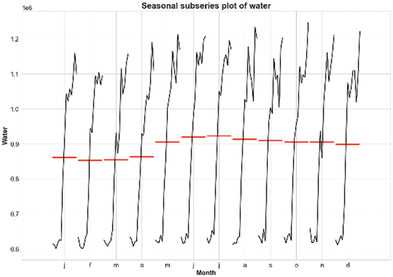
Figure 4: The seasonal subseries plot of water demand

The next step is the normalization of inputs. We use the min-max method because it provides high performance. Further details about normalization can be found through the reference [10]. Then, we convert our time series into a supervised learning dataset. The observations of time series are interdependent. We used a sequence of past observations (X) to forecast sequence values (Y) [47]. Then, we use the value (Y) as input for the next prediction and so on, as shown in Eq. (1). So, we divide the dataset into the sequence of inputs (called input layer) and sequence of outputs. In this paper, we forecast next week so the sequence of output is seven values.

Y=f(X)(1)

3.3 Artificial Neural Network (ANN)

Artificial Neural Networks are based on brain-inspired principles. In fact, ANN is able to analyze and extract complex non-linear relationships. ANN is very useful to solve complex problems such as forecasting. In forecasting, three models are extensively deployed. These models are MLP, Recurrent Neural Network (RNN) and Radial Basis Function Neural Network (RBF) [9].

In this work, we used MLP to predict water demand. The architecture (as shown in Fig. 5) and hyperparameters (as shown in Tab. 2) can be trained using a backpropagation algorithm. In this algorithm, the input training pattern is fed-forward, errors are calculated and backpropagated, and the synapses are weighted accordingly [48,49]. The backpropagation algorithm is useful for learning complex and large-scale problems [50]. During training, the amount controlling weight update is called the learning rate (η). The structure of MLP contains three layers. It contains the input, the hidden and the output layers. The output layer has seven neurons to predict the next 7 days (as called multi-step time series forecasting).

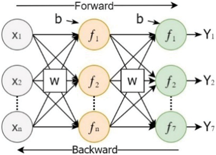
Figure 5: The structure of MLP

Then, we select the best activation function. The most common type of activation function used in hidden layers is sigmoid. Another common type is the Rectified Linear Unit (ReLU). The most common types of activation function used in the output layer are the ReLU and linear (see Fig. 6).

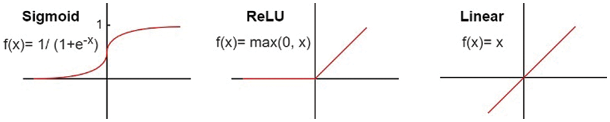
Figure 6: The activation functions for hidden and output layers

Also, we select the best optimizer (i.e., adam, adamax…) and the η used for adjusting weights of the synapses. Training is repeated till a certain number of iterations (example: 1000 epochs) and stopped when the model’s performance cannot be improved or reaches a minimum error. Finally, we evaluate the final model using walk-forward validation. It predicts one step and evaluates the result against the known value using RMSE, then it stores for the next prediction. This process will be repeated finishing all the testing data. Although its computational cost is high because it moves one step through the time series, it is robust for time series forecasting [47]. The output y^ of MLP model can be calculated by Eq. (2).

y^=f(b+∑k=1nwkxk)(2)

where, f(.) is the activation function, b is the bias, w are weights (w1,…,wn) and x are inputs from 1 to n neurons (x1,…,xn). The weight is updated using optimization techniques (i.e., adam) and the η. To evaluate the performance of a model, we use RMSE metric calculated as in Eq. (3):

RMSE=1n∑x=1n(yx−y^x)2(3)

where, n is the number of historical data (x index varying from 1 to n), yx is the actual value and y^x is the forecasted value.

3.4 Particle Swarm Optimization (PSO)

In 1995, Kennedy and Eberhart presented a particle search algorithm that mimics the behavior of fish and birds [51]. There are several candidates for the optimal solution, each of which is driven by individual search (cognitive search) and global search (social search) to minimize the error function shown in Eq. (4).

minf(x)(4)

Each particle has a position denoted by xiϵRn, i=1,..,n, where n is the number of particles. Also, it has a velocity denoted by viϵRn. Finally, each particle has a fitness value to evaluate its quality. So, during the search process and over each iteration (t), particles move according to Eq. (5).

x(t+1)i=x(t)i+v(t+1)i(5)

where, x denotes the position of particles. i denotes the number of particles. t is the current iteration. The velocity v(t+1)i is adjusted according to Eq. (6).

v(t+1)i=ωv(t)i+C1r1(p(t)i−x(t)i)+C2r2(g(t)i−x(t)i)(6)

where,

•   ω is inertia weight, the common value is: ω = 0.7298,

•   C1 and C2 are cognition learning factor and social learning rate, respectively. The common value is: C1=C2 = 1.49618,

•   r1 and r2 are uniformly random numbers in [0,1],

•   p(t)i and g(t)i are the best personal and global solutions, respectively.

Tab. 3 represents PSO’s hyperparameters used in our work. In this study, we try the model’s effectiveness using population (size = 20) and number of iterations (50).

3.5 Multivariate Time Series Forecasting Using PSO-ANN

In this section, a mapping between PSO and ANN is established. As mentioned before the multi-step forecasting of time series can be modeled using MLP. The MLP model defined in Eq. (2) can be mapped to PSO. Hence, the vector’s position is defined according to Eq. (7):

xi=[f(.)1i,f(.)2i,ni,wi,ηi](7)

where, f(.)1 : is the activation function of the hidden layer. f(.)2: is the activation function of the output layer. n is the number of neurons in the hidden layer and η is the learning rate. The best optimization w is responsible for adjusting weights. The quality of these particles is evaluated according to the fitness function defined in Eq. (8).

f(xi)=∑z=1n(y(z)−y^(z))2(8)

where, y^(z) is calculated according to Eq. (9):

y^(z)=f(i)(b+∑k=1n(i)wk(i)xk(i))(9)

Fig. 7 shows steps followed to predict water needs under the impact of climatic conditions using PSO-ANN. These steps can be detailed as follows:

1.    Load the data of water demand and climatic conditions from 2004 to 2018.

2.    Pre-process the dataset (make it stationary, remove leap year, normalize, and convert time series to a supervised learning).

3.    Implement the naïve approach to compare its results with those obtained in PSO-ANN.

4.    Specify PSO’s hyperparameters (Tab. 3).

5.    Specify MLP’s hyperparameters (i.e., number of epochs in Tab. 2).

6.    Assign t=1 for the first iteration.

7.    Initialize particles randomly (Tab. 2 and Eq. (7))

8.    Evaluate each particle according to equations Eqs. (8) and (9), then update the personal best (p(t)i) for each particle and the global best (g(t)i) for the entire population.

9.    Increment the iteration: t=t+1.

10.   Update the position of each particle using Eqs. (5) and (6).

11.   Update activation functions, the number of hidden neurons, η, and w.

12.   Compute the fitness function for each particle using Eqs. (8) and (9).

13.   Compare the current fitness function to its previous. If the current is improved, then set p(t)i=x(t)i.

14.   Determine and update the global best particle in the swarm (g(t)i).

15.   Repeat from step (9) until reaching the max iteration, then output the (g(t)i) as the best solution.

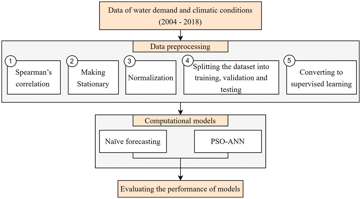
Figure 7: The methodology of multivariate time series forecasting

4  Results and Discussion

For implementation, we used Python language. In the following subsections, we show results after making our series stationary, results of naïve forecasting, and results of multivariate time series forecasting using PSO-ANN.

4.1 Making Our Series Stationary

As mentioned in Sub-Section 3.2, we firstly determine the most climate factors correlated with water demand using Spearman’s correlation. The result shows that the dew point is the most factor affecting water demand, then min, avg and max temperature by 0.155, 0.151, 0.137 and 0.144 respectively, as shown in Fig. 2. Then we make our time series stationary by removing trend from water demand and seasonality from climatic conditions (see Fig. 8). Now, our time series is ready to be modeled.

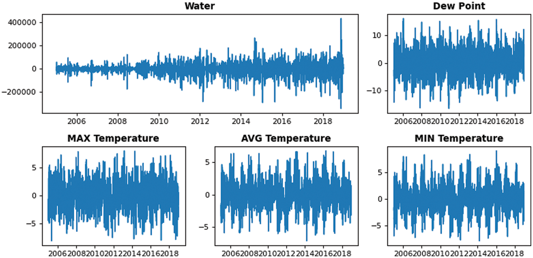
Figure 8: Line plot for our time series after making it stationary

4.2 Results of Naïve Forecasting

Naïve forecasting is usually used as a baseline for performance’s evaluation. It can be very helpful for improving the proposed model. So, we do three experiments for forecasting the next seven days. We evaluate the forecasting for each day separately and also over all days. Our three experiments used the last day prior (one past day is called daily), the prior week (seven past days is called weekly), and the same week for the last year (seven past days of the last year is called week-yearly). This step is helpful to determine the best number of inputs used for forecasting. Tab. 4 and Fig. 9 show results of naïve forecasting. Tab. 4 shows that, in the first row, we obtain the best performance for all days. Also, the 1st day provided accurate forecasting rather than other days. As shown in Fig. 9, the error of week-yearly is very large, but there is a similarity between daily and weekly. The error rate is similar on the 7th day. Also, we consider for the daily curve that the 1st day is the accurate day for forecasting, unlike the 5th day, which is the worst one.

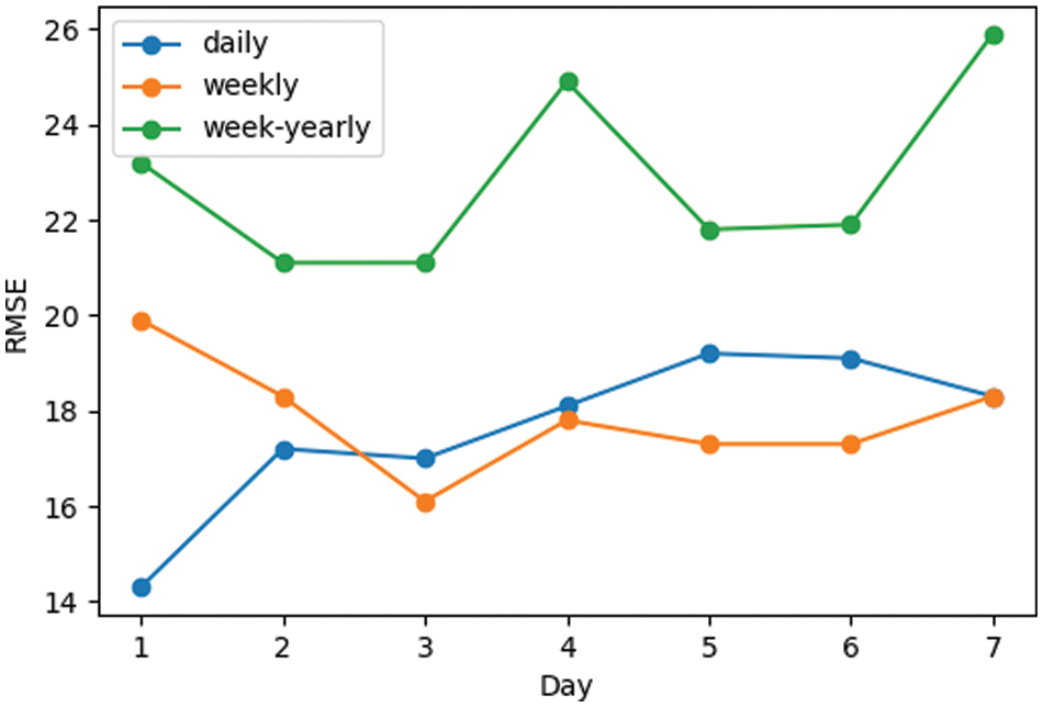
Figure 9: Naïve forecasting

4.3 Results of Multivariate Time Series Forecasting Using PSO-ANN

Tab. 5 shows a comparison between the naïve approach and PSO-ANN. The performance’s prediction has been improved from 17.5 to 11.6. The second day is the easiest day to predict (lowest error), while the first day is the most difficult day to predict (highest error).

The line plot for RMSE using naïve and PSO-ANN is shown in Fig. 10. The RMSE of the 1st day closes in both models. For the following days, the error using the naïve approach increases over time, whereas it decreases when using PSO-ANN. As shown in the PSO-ANN curve, the 1st day has the highest error while the 2nd day has the lowest error and can be considered the accurate day for forecasting. Then, the error increases again on the 3rd day and decreases in the following two days. Finally, it increases and becomes stable during the last two days.

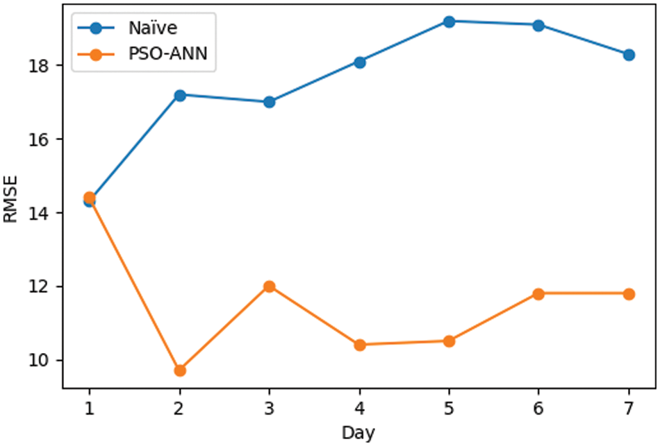
Figure 10: Comparison between the naïve approach and PSO-ANN forecasting

Hence, we use PSO-ANN to predict daily water needs while considering the impact of climatic conditions. Fig. 11 depicts the number of days used on training, validation, testing, and prediction. However, Fig. 12 illustrates a zoomed-in view of the testing and prediction. It indicates that prediction values are closely following testing values.

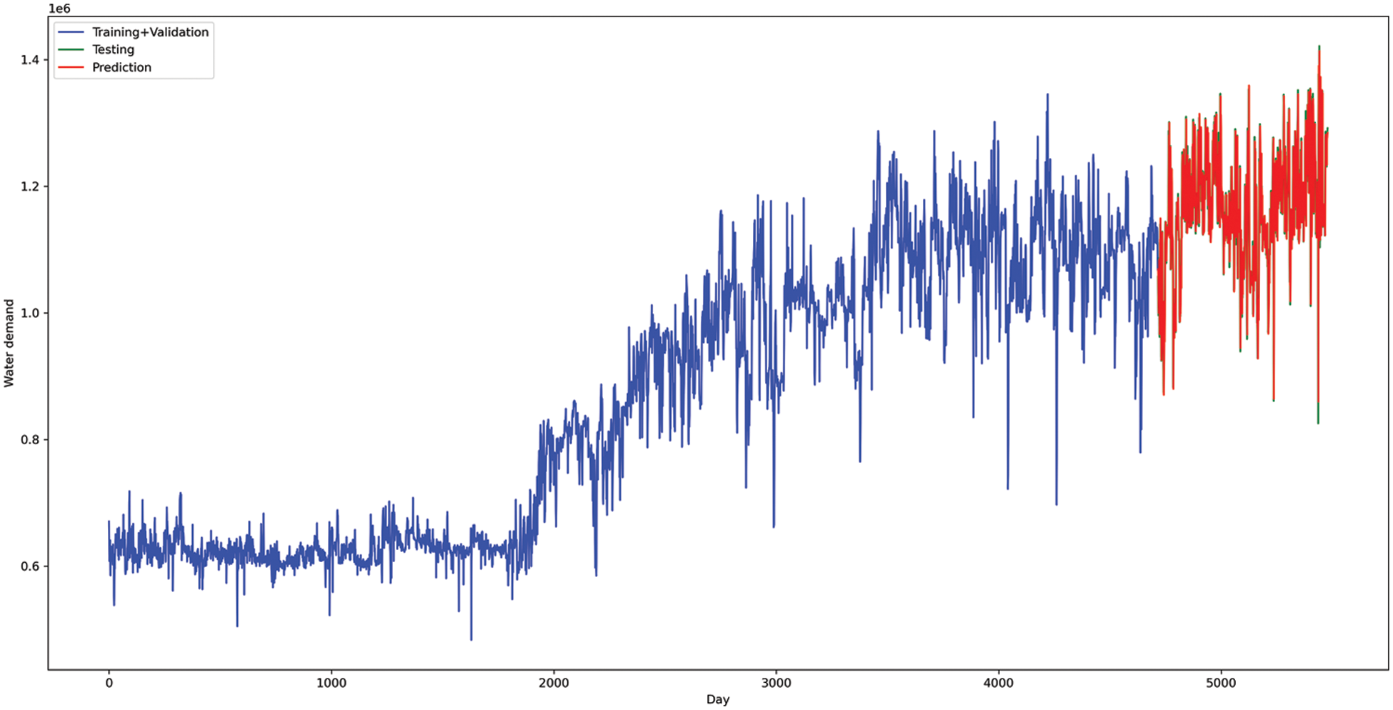
Figure 11: PSO-ANN forecasting

Figure 12: A zoomed-in view of PSO-ANN forecasting

We can conclude that the PSO-ANN’s performance is effective. Hence, our hybrid model can be generalized to be used in a multitude of multivariate time series problems. This work used PSO to tune ANN’s hyperparameters instead of using a traditional grid random search algorithm.

5  Conclusion

Throughout our work, we developed a hybrid model for forecasting daily water needs while considering climatic conditions. The historical data was collected in the period (2004–2018) in Jeddah city, Saudi Arabia. Then, we study the relationship between water demand and climatic conditions using Spearman’s correlation. After that, we pre-processed the multivariate time series in order to make it stationary by removing trend and seasonality. We used the min-max for normalization and converted it to supervised learning. Then, we used ANN for forecasting the future, PSO for tuning ANN’s hyperparameters and the naïve approach for comparison. Finally, we provided the hybrid model called PSO-ANN to predict water needs under the impact of climatic conditions. Walk-forward validation has been used for evaluating PSO-ANN. Results showed PSO-ANN is an accurate model and reliable for forecasting. In fact, PSO-ANN outperformed the naïve approach. The RMSE in PSO-ANN is equal to 11.6 while it is equal to 17.5 in the naïve approach. Also, results showed that the RMSE on the first day is the biggest, while the RMSE on the second day is the smallest. Finally, results showed that the dew point is the most climatic condition affecting water demand. Future work can investigate other extensively used techniques such as genetic algorithm or any other evolutionary algorithms for ANN’s hyperparameters tuning.

Acknowledgement: We are deeply grateful to the General Directorate of Water in Jeddah, Saudi Arabia for providing us with the historical water consumption.

Funding Statement: The authors received no specific funding for this study.

Conflicts of Interest: The authors declare that they have no conflicts of interest to report regarding the present study.

References

 1.  N. T. Graham, M. I. Hejazi, M. Chen, E. G. Davies, J. A. Edmonds et al., “Humans drive future water scarcity changes across all Shared Socioeconomic Pathways,” Environmental Research Letters, vol. 15, no. 1, pp. 014007, 2020. [Google Scholar]

 2.  M. Flörke, C. Schneider and R. I. McDonald, “Water competition between cities and agriculture driven by climate change and urban growth,” Nature Sustainability, vol. 1, no. 1, pp. 51–58, 2018. [Google Scholar]

 3.  I. Haddeland, J. Heinke, H. Biemans, S. Eisner, M. Flörke et al., “Global water resources affected by human interventions and climate change,” Proceedings of the National Academy of Sciences, vol. 111, no. 9, pp. 3251–3256, 2014. [Google Scholar]

 4.  J. Schewe, J. Heinke, D. Gerten, I. Haddeland, N. W. Arnell et al., “Multimodel assessment of water scarcity under climate change,” Proceedings of the National Academy of Sciences, vol. 111, no. 9, pp. 3245–3250, 2014. [Google Scholar]

 5.  T. I. E. Veldkamp, Y. Wadab, H. de Moela, M. Kummuc, S. Eisner et al., “Changing mechanism of global water scarcity events: Impacts of socioeconomic changes and inter-annual hydro-climatic variability,” Global Environmental Change, vol. 32, no. 2, pp. 18–29, 2015. [Google Scholar]

 6.  E. DeNicola, O. S. Aburizaiza, A. Siddique, H. Khwaja and D. O. Carpenter, “Climate change and water scarcity: The case of Saudi Arabia,” Annals of Global Health, vol. 81, no. 3, pp. 342–353, 2015. [Google Scholar]

 7.  Saline Water Conversion Corporation, The annual report of the saline water conversion corporation, 2019. [Online]. Available: https://www.swcc.gov.sa/uploads/ANNUAL_REPORT_2019.pdf. [Google Scholar]

 8.  Ministry of Environment Water and Agriculture, Saudi national water strategy 2030, 2018. [Online]. Available: https://الاستراتيجيةالوطنيةللمياه2030.pdf(mewa.gov.sa). [Google Scholar]

 9.  G. Nalcaci, A. Özmen and G. W. Weber, “Long-term load forecasting: Models based on MARS, ANN and LR methods,” Central European Journal of Operations Research, vol. 27, no. 4, pp. 1033–1049, 2019. [Google Scholar]

10. A. B. Al-Ghamdi, S. Kamel and M. Khayyat, “Evaluation of artificial neural networks performance using various normalization methods for water demand forecasting,” in 2021 National Computing Colleges Conf. (NCCC), Taif, Saudi Arabia, IEEE, pp. 1–6, 2021. [Google Scholar]

11. O. I. Abiodun, A. Jantan, A. E. Omolara, K. V. Dada, N. A. Mohamed et al., “State-of-the-art in artificial neural network applications: A survey,” Heliyon, vol. 4, no. 11, pp. e00938, 2018. [Google Scholar]

12. H. Kukreja, N. Bharath, C. S. Siddesh and S. Kuldeep, “An introduction to artificial neural network,” International Journal of Advance Research and Innovative Ideas in Education, vol. 1, pp. 27–30, 2016. [Google Scholar]

13. I. N. da Silva, D. H. Spatti, R. A. Flauzino, L. H. B. Liboni and S. F. dos Reis Alves, “Multilayer perceptron networks,” in Artificial Neural Networks. Cham: Springer, pp. 55–115, 2017. [Google Scholar]

14. A. Altunkaynak and T. A. Nigussie, “Monthly water demand prediction using wavelet transform, first-order differencing and linear detrending techniques based on multilayer perceptron models,” Urban Water Journal, vol. 15, no. 2, pp. 177–181, 2018. [Google Scholar]

15. N. Rasifaghihi, S. S. Li and F. Haghighat, “Forecast of urban water consumption under the impact of climate change,” Sustainable Cities and Society, vol. 52, no. 10, pp. 101848, 2020. [Google Scholar]

16. Y. Seo, S. Kwon and Y. Choi, “Short-term water demand forecasting model combining variational mode decomposition and extreme learning machine,” Hydrology, vol. 5, no. 4, pp. 54, 2018. [Google Scholar]

17. Y. Yang, Q. Xiong, C. Wu, Q. Zou, Y. Yu et al., “A study on water quality prediction by a hybrid CNN-LSTM model with attention mechanism,” Environmental Science and Pollution Research, vol. 28, no. 39, pp. 55129–55139, 2021. [Google Scholar]

18. G. Marcjasz, “Forecasting electricity prices using deep neural networks: A robust hyper-parameter selection scheme,” Energies, vol. 13, no. 18, pp. 4605, 2020. [Google Scholar]

19. M. Ahmad, J. L. Hu, M. Hadzima-Nyarko, F. Ahmad, X. W. Tang et al., “Rockburst hazard prediction in underground projects using two intelligent classification techniques: A comparative study,” Symmetry, vol. 13, no. 4, pp. 632, 2021. [Google Scholar]

20. X. Zhang, L. Yao, C. Huang, Q. Z. Sheng and X. Wang, “Intent recognition in smart living through deep recurrent neural networks,” in Int. Conf. on Neural Information Processing, Cham, Springer, vol.10635, pp. 748–758, 2017. [Google Scholar]

21. J. Bergstra, R. Bardenet, Y. Bengio and B. Kégl, “Algorithms for hyper-parameter optimization,” Advances in Neural Information Processing Systems, vol. 24, pp. 2546–2554, 2011. [Google Scholar]

22. D. Wang, D. Tan and L. Liu, “Particle swarm optimization algorithm: An overview,” Soft Computing, vol. 22, no. 2, pp. 387–408, 2018. [Google Scholar]

23. A. Haidar, M. Field, J. Sykes, M. Carolan and L. Holloway, “PSPSO: A package for parameters selection using particle swarm optimization,” SoftwareX, vol. 15, no. Supplement C, pp. 100706, 2021. [Google Scholar]

24. X. J. Wang, J. Y. Zhang, S. Shamsuddin, R. L. Oyang, T. S. Guan et al., “Impacts of climate variability and changes on domestic water use in the Yellow River Basin of China,” Mitigation and Adaptation Strategies for Global Change, vol. 22, no. 4, pp. 595–608, 2017. [Google Scholar]

25. X. J. Wang, J. Y. Zhang, S. Shahid, S. H. Bi, A. Elmahdi et al., “Forecasting industrial water demand in Huaihe River Basin due to environmental changes,” Mitigation and Adaptation Strategies for Global Change, vol. 23, no. 4, pp. 469–483, 2018. [Google Scholar]

26. K. Alotaibi, A. R. Ghumman, H. Haider, Y. M. Ghazaw and M. Shafiquzzaman, “Future predictions of rainfall and temperature using GCM and ANN for arid regions: A case study for the Qassim Region, Saudi Arabia,” Water, vol. 10, no. 9, pp. 1260, 2018. [Google Scholar]

27. A. E. M. Al-Juaidi and A. S. Al-Shotairy, “Evaluation of municipal water supply system options using water evaluation and planning system (WEAPJeddah case study,” Desalination and Water Treatment, vol. 176, pp. 317–323, 2020. [Google Scholar]

28. J. F. Farfán, K. Palacios, J. Ulloa and A. Avilés, “A hybrid neural network-based technique to improve the flow forecasting of physical and data-driven models: Methodology and case studies in Andean watersheds,” Journal of Hydrology: Regional Studies, vol. 27, pp. 100652, 2020. [Google Scholar]

29. S. Chowdhury, M. Al-Zahrani and A. Abbas, “Implications of climate change on crop water requirements in arid region: An example of Al-Jouf,” Saudi Arabia, Journal of King Saud University-Engineering Sciences, vol. 28, no. 1, pp. 21–31, 2016. [Google Scholar]

30. R. A. Vozhehova, Y. O. Lavrynenko, S. V. Kokovikhin, P. V. Lykhovyd, I. M. Biliaieva et al., “Assessment of the CROPWAT 8.0 software reliability for evapotranspiration and crop water requirements calculations,” Journal of Water and Land Development, vol. 39, no. 1, pp. 147–152, 2018. [Google Scholar]

31. S. L. Zubaidi, P. Kot, R. M. Alkhaddar, M. Abdellatif and H. Al-Bugharbee, “Short-term water demand prediction in residential complexes: Case study in Columbia city, USA,” in 2018 11th Int. Conf. on Developments in eSystems Engineering (DeSE), Cambridge, UK, IEEE, pp. 31–35, 2018. [Google Scholar]

32. P. Huntra and T. C. Keener, “Evaluating the impact of meteorological factors on water demand in the Las Vegas Valley using time-series analysis: 1990—2014,” ISPRS International Journal of Geo-Information, vol. 6, no. 8, pp. 249, 2017. [Google Scholar]

33. P. Vijai and P. B. Sivakumar, “Performance comparison of techniques for water demand forecasting,” Procedia Computer Science, vol. 143, no. 2, pp. 258–266, 2018. [Google Scholar]

34. M. Narvekar, P. Fargose and D. Mukhopadhyay, “Weather forecasting using ANN with error backpropagation algorithm,” in Proc. of the Int. Conf. on Data Engineering and Communication Technology, Singapore, Springer, vol.468, pp. 629–639, 2017. [Google Scholar]

35. O. Oyebode, “Evolutionary modelling of municipal water demand with multiple feature selection techniques,” Journal of Water Supply: Research and Technology-Aqua, vol. 68, no. 4, pp. 264–281, 2019. [Google Scholar]

36. A. Ajbar and E. M. Ali, “Prediction of municipal water production in touristic Mecca City in Saudi Arabia using neural networks,” Journal of King Saud University-Engineering Sciences, vol. 27, no. 1, pp. 83–91, 2015. [Google Scholar]

37. M. A. Al-Zahrani and A. Abo-Monasar, “Urban residential water demand prediction based on artificial neural networks and time series models,” Water Resources Management, vol. 29, no. 10, pp. 3651–3662, 2015. [Google Scholar]

38. S. L. Zubaidi, S. Ortega-Martorell, P. Kot, R. M. Alkhaddar, M. Abdellatif et al., “A method for predicting long-term municipal water demands under climate change,” Water Resources Management, vol. 34, no. 3, pp. 1265–1279, 2020. [Google Scholar]

39. Y. Lu, Y. Zhou and X. Wu, “A hybrid lightning search algorithm-simplex method for global optimization,” Discrete Dynamics in Nature and Society, vol. 2017, pp. 1–23, 2017. [Google Scholar]

40. S. L. Zubaidi, S. Ortega-Martorell, H. Al-Bugharbee, I. Olier, K. S. Hashim et al., “Urban water demand prediction for a city that suffers from climate change and population growth: Gauteng province case study,” Water, vol. 12, no. 7, pp. 1885, 2020. [Google Scholar]

41. F. Zou, D. Chen and R. Lu, “Hybrid hierarchical backtracking search optimization algorithm and its application,” Arabian Journal for Science and Engineering, vol. 43, no. 2, pp. 993–1014, 2018. [Google Scholar]

42. M. Hasanipanah, M. Noorian-Bidgoli, D. J. Armaghani and H. Khamesi, “Feasibility of PSO-ANN model for predicting surface settlement caused by tunneling,” Engineering with Computers, vol. 32, no. 4, pp. 705–715, 2016. [Google Scholar]

43. P. Panyadee, P. Champrasert and C. Aryupong, “Water level prediction using artificial neural network with particle swarm optimization model,” in 2017 5th Int. Conf. on Information and Communication Technology (ICoIC7), Melaka, Malaysia, IEEE, pp. 1–6, 2017. [Google Scholar]

44. D. T. Viet, V. Van Phuong, M. Q. Duong and Q. T. Tran, “Models for short-term wind power forecasting based on improved artificial neural network using particle swarm optimization and genetic algorithms,” Energies, vol. 13, no. 11, pp. 2873, 2020. [Google Scholar]

45. NASA, “Power data access viewer,” 2020. [Online]. Available: https://power.larc.nasa.gov/data-access-viewer/. [Google Scholar]

46. J. Brownlee, “How to calculate correlation between variables in Python,” Machine Learning Mastery, 2020. [Online]. Available: https://machinelearningmastery.com/how-to-use-correlation-to-understand-the-relationship-between-variables/. [Google Scholar]

47. J. Brownlee, Introduction to time series forecasting with python: How to prepare data and develop models to predict the future. Vermont, Victoria, Australia: Machine Learning Mastery, 2017. [Online] Available https://books.google.de/books?id=-AiqDwAAQBAJ&source=gbs_books_other_versions. [Google Scholar]

48. J. Tarigan, Nadia, R. Diedan and Y. Suryana, “Plate recognition using backpropagation neural network and genetic algorithm,” Procedia Computer Science, vol. 116, no. 3, pp. 365–372, 2017. [Google Scholar]

49. S. P. Siregar and A. Wanto, “Analysis of artificial neural network accuracy using backpropagation algorithm in predicting process (forecasting),” IJISTECH (International Journal of Information System & Technology), vol. 1, no. 1, pp. 34–42, 2017. [Google Scholar]

50. A. Ehret, D. Hochstuhl, D. Gianola and G. Thaller, “Application of neural networks with back-propagation to genome-enabled prediction of complex traits in Holstein-Friesian and German Fleckvieh cattle,” Genetics Selection Evolution, vol. 47, no. 1, pp. 1–9, 2015. [Google Scholar]

51. J. Kennedy and R. Eberhart, “Particle swarm optimization,” in Proc. of ICNN’95-Int. Conf. on Neural Networks, Perth, WA, Australia, IEEE, vol.4, pp. 1942–1948, 1995. [Google Scholar]

This work is licensed under a Creative Commons Attribution 4.0 International License, which permits unrestricted use, distribution, and reproduction in any medium, provided the original work is properly cited.