Computers, Materials & Continua DOI:10.32604/cmc.2022.026771
Article

A TMA-Seq2seq Network for Multi-Factor Time Series Sea Surface Temperature Prediction

Qi He1, Wenlong Li1, Zengzhou Hao2, Guohua Liu3, Dongmei Huang1, Wei Song1,*, Huifang Xu4, Fayez Alqahtani5 and Jeong-Uk Kim6

1Department of Information Technology, Shanghai Ocean University, Shanghai, 201306, China
2State Key Laboratory of Satellite Ocean Environment Dynamics, Second Institute of Oceanography, Ministry of Natural Resources, Hangzhou, 310012, China
3College of Computer, Dong Hua University, Shanghai, 200051, China
4College of Information Technology, Shanghai Jian Qiao University, Shanghai, 201306, China
5Software Engineering Department, College of Computer and Information Sciences, King Saud University, Riyadh 12372, Saudi Arabia
6Department of Electrical Engineering, Sangmyung University, South Korea, Korea
*Corresponding Author: Wei Song. Email: wsong@shou.edu.cn
Received: 04 January 2022; Accepted: 02 March 2022

Abstract: Sea surface temperature (SST) is closely related to global climate change, ocean ecosystem, and ocean disaster. Accurate prediction of SST is an urgent and challenging task. With a vast amount of ocean monitoring data are continually collected, data-driven methods for SST time-series prediction show promising results. However, they are limited by neglecting complex interactions between SST and other ocean environmental factors, such as air temperature and wind speed. This paper uses multi-factor time series SST data to propose a sequence-to-sequence network with two-module attention (TMA-Seq2seq) for long-term time series SST prediction. Specifically, TMA-Seq2seq is an LSTM-based encoder-decoder architecture facilitated by factor- and temporal-attention modules and the input of multi-factor time series. It takes six-factor time series as the input, namely air temperature, air pressure, wind speed, wind direction, SST, and SST anomaly (SSTA). A factor attention module is first designed to adaptively learn the effect of different factors on SST, followed by an encoder to extract factor-attention weighted features as feature representations. And then, a temporal attention module is designed to adaptively select the hidden states of the encoder across all time steps to learn more robust temporal relationships. The decoder follows the temporal-attention module to decode the feature vector concatenated from the weighted features and original input feature. Finally, we use a fully-connect layer to map the feature into prediction results. With the two attention modules, our model effectively improves the prediction accuracy of SST since it can not only extract relevant factor features but also boost the long-term dependency. Extensive experiments on the datasets of China Coastal Sites (CCS) demonstrate that our proposed model outperforms other methods, reaching 98.29% in prediction accuracy (PACC) and 0.34 in root mean square error (RMSE). Moreover, SST prediction experiments in China’s East, South, and Yellow Sea site data show that the proposed model has strong robustness and multi-site applicability.

Keywords: Sea surface temperature; multi-factor; attention; long short-term memory

1  Introduction

Sea surface temperature (SST) is one of the important parameters in the global atmospheric system. In recent years, with great attention attached to ocean climate, ocean environmental protection [1], fisheries [2], and other ocean-related fields [3], accurately predicting SST has become a hot research topic. So far, researchers have proposed many methods to predict SST, which can be classified into two categories. One category is known as the numerical prediction based on oceanography physics [4–6], which uses a series of complex physical equations to describe SST variation rules. Another category is data-driven models such as support vector machine (SVM) [7] and artificial neural network (ANN) [8], which automatically learn the SST change trend from SST data. With a huge amount of ocean monitoring data being continually collected, the data-driven methods for SST time-series prediction show promising results [9–11].

Recently, data-driven research and model has been widely applied in medicine [12,13], finance [14,15], and privacy security [16], and achieved great success. But multi-factor time series data-driven modeling is still an important but complex problem in many fields, such as wind speed prediction [17], and energy and indoor temperature prediction [18]. For SST, it is affected by complex ocean environmental factors. He et al. [19] measured the correlation between ocean environmental factors, and the results showed that SST is closely related to various factors such as wind speed and air temperature. Therefore, using multi-factor time series SST data, can effectively extract the influence of physical mechanisms on SST through model learning and improve the applicability in different sea areas to achieve more accurate SST prediction. However, SST prediction of long-term and multi-factor time series is still a challenging problem, mainly reflected in the feature representation and selection mechanism of relationships between different series.

SST data are long-term data series, typically involving large data volumes. Many scholars regard SST prediction as a time series regression problem and propose many time series methods to predict SST. For example, the autoregressive integrated moving average (ARIMA) model [20] focuses on seasonality and regularity, while cannot express nonlinear correlations. Recurrent neural network (RNN) [21] is a neural network specialized in time series modeling. However, traditional RNN is prone to the problem of gradient disappearance when it processes long-term time series [22]. Therefore, the time series prediction model based on RNN is rarely used in SST prediction. But long short-term memory(LSTM) [23] has strong time series modeling capability over short or long time periods, it uses recurrently connected cells to learn dependencies between them, and then transfer the learned parameters to the next cells, so it has attained a huge success in a variety of tasks, such as image processing [24], machine translation [25] and speech recognition [26]. Qin et al. [27] first used the LSTM model to solve SST prediction problems. However, the vectorization of simultaneous factors w/o the factor selection cannot extract correlation between different factors.

Recently, the advances in LSTM models have provided more frameworks for dealing with series prediction problems. Sequence-to-sequence (Seq2seq) structure is one of the encoder-decoder networks. The key idea is to encode the input series as feature representation and use the decoder to generate the results. This structure has been widely used in machine translation [28]. However, the performance of an encoder-decoder network will deteriorate rapidly as the length of the input series increases [29]. Therefore, some researchers have introduced attention mechanisms into the encoder-decoder networks. Attention mechanism can better select the important feature information in the network to improve the information processing capabilities of neural multi-order.

In recent years, attention mechanisms have been widely used and perform well in many different types of deep learning tasks [30,31]. Bahdanau et al. [32] used an attention mechanism to select parts of hidden states across all the time steps in the encoder-decoder network. Based on this, Luong et al. [33] proposed an encoder-decoder network based on a global attention mechanism. Qin et al. [34] proposed a dual-stage attention-based recurrent neural network (DA-RNN). It was applied to predict target series through input and temporal attention, achieving a good prediction performance. The method provides a new idea for multi-factor time series SST prediction.

Existing SST prediction models have not taken into consideration complex interactions between SST and other ocean factors and have the problem of performance degradation as the length of the input series increases. To achieve high accuracy of SST prediction, in this paper, we present a multi-factor time series SST prediction model, which is constructed as an LSTM-based encoder-decoder network with a two-module of attention, named TMA-Seq2seq. The introduced attention module can quantitatively assign an importance weight to each specific factor and every time step of the series features, which ameliorates the attentional dispersion defects of the traditional LSTM.

The main contributions of this paper are as follows:

(1)   Considering the potential impact of other ocean factors on SST, we propose a factor attention module to adaptively learn the effect of different factors on SST according to attention weight. In addition, we also design a new factor SST anomaly (SSTA) extracted from an SST time series, which can effectively enrich the feature representation information.

(2)   To improve the poor performance in long-term time series data prediction, we propose a temporal attention module to extract long-term time information, which can select hidden states of the encoder across all time steps to learn more robust temporal relationships.

(3)   To solve the low accuracy of the model for different sea areas SST prediction, we combine the original features of data and weighted features as the input of decoder, which can effectively retain the underlying features of the data and improve the robustness of the model.

In summary, our work provides a new SST prediction model, which significantly improves the prediction accuracy. We achieve this goal via the factor and temporal attention module, which is responsible for reaching 98.29% in prediction accuracy (PACC) 0.34 in root mean square error (RMSE). Besides, the SST prediction experiments in different sea areas validate the strong robustness of the proposed method.

2  Proposed Models

2.1 TMA-Seq2seq Model

The overall framework of the proposed TMA-Seq2seq model is illustrated in Fig. 1. It includes data preprocessing, factor attention module, LSTM-based encoder, temporal attention module and LSTM decoder. The main steps of the model are as follows:

①   Data preprocessing. Wu et al. [35] analyzed the characteristics of the interannual variation of SST anomaly (SSTA) in the Bohai Sea region and found that the variation of SST anomaly is the most direct manifestation of the influence of ocean anomalies phenomenon on SST. However, SST within a small time window cannot represent the interannual variation of SST. Therefore, we add a new factor SSTA to indicate the relative difference of current SST to the annual average of SST. The time series of the SSTA factor is computed by (1). Let a be the vector of original SST time series a=(a1,…,at−1,…,aT), and T is the total length of the SST series. We first calculate two feature vectors a¯ and σ, which represent the mean value and the standard deviation of an annual cycle, respectively. Then, we calculate the vector a∗ to represent the difference of SST and interannual mean variation for every time step and take it as the SSTA factor. After data preprocessing, the input of multi-factor time series is X=(x1,…,xk,…,xn)=(x1,…,xt−1,…,xT)T∈Rn×T, T is the size of time window, n is the number of factors. a∗=a−a¯σ(1)

②   Factor attention module. In the time window l, the multi-factor time series X is the input of the module. And then, we get a factor-attention vector αl=(α1l,…,αkl,…,αnl)∈Rn and multiply it with the corresponding input time series. Finally, we transpose the weighted feature series and obtain the vector X′=(x1′,…,xt′,…,xT′)∈RT×n, thereby better maintaining time dependency.

③   LSTM-based encoder. We use a single layer of LSTM to encode the weighted feature series X′. Then, we get the hidden state of all the time step hl=(h1l,…,htl,…,hTl)∈RT×m, m is the hidden size of the encoder.

④   Temporal attention module. The feature representation hl is the input of the module. At the time t, the temporal-attention weight is βt=(β1t,…,βtt,…,βTt)∈RT. And then, we multiply the corresponding hidden state and obtain the weighted summed feature xt−1′′ at time t. Finally, we obtain the new vector X′′=(x1′′,…,xt−1′′,…,xT′′)∈RT×m.

⑤   LSTM-based decoder. We use another layer of LSTM to decode the feature vector concatenated from the temporal-attention weighted feature X′′ and original input feature XT. Then, we get the output cT∈Rp of the model, p the hidden size of the decoder. Finally, we use the full connection layer (FC-Layer) to map cT to the final prediction result y^.

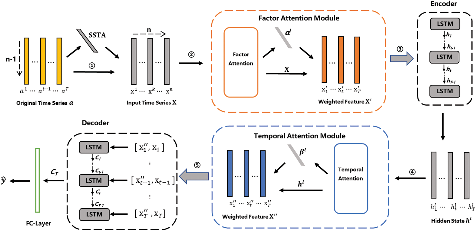
Figure 1: The overall framework of the proposed TMA-Seq2seq model

For SST prediction modeling, given the previous values of the input time series X∈Rn×T. We aim to predict the future SST values over next d time steps, denoted as y^=(y^T+1,y^T+2,…,y^T+d)∈Rd, which is shown as follow:

y^=f(x1,…,xk,…,xn)(2)

where f(⋅) is a nonlinear mapping function we aim to learn.

2.2 Factor Attention Module

The Initial letter of each notional word in all headings is capitalized. We design a factor attention module for learning the effect of different factors on SST. This is inspired by machine translation work, where the global attention mechanism aligns the relationship between target words and source words.

A graphical illustration of the factor attention module is shown in Fig. 2. We first take the input series X as the input feature of the module. And we only use the dot product of factor feature vector to calculate the attention weight of all factors. SST feature vector is an important role of the calculation of attention weight, i.e., target feature xk. Then, the factor attention score for every factor el=(e1l,…,ekl,…,enl)∈Rn is calculated by (3), which establishes the relationship between the target factor SST and every other factor. Next, a softmax function is used to map the attention score ek into the factor attention weight αk, which represents the impacts of the factor in time series prediction. The factor relationships can be learned by an attention mechanism as follows:

el=XWe(xk)T(3)

αkl=exp(ekl)∑i=1n⁡exp(eil)(4)

where We∈Rp×p is the parameter to learn. Finally, these factor attention weights αl=(α1l,…,αkl,…,αnl) are multiplied by the corresponding input series X and get the weighted feature X′. It will be used as the input of the encoder to further extract the time feature. The output after the factor attention module is defined as follows:

X′=(x1α1l,…,xkαkl,…,xnαnl)T=(x1′,…,xt′,…,xT′)(5)

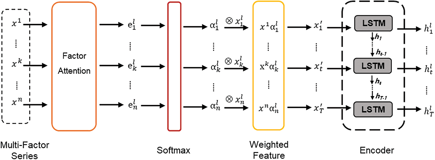
Figure 2: A graphical illustration of the factor attention module

2.3 Temporal Attention Module

Considering that the performance of the encoder-decoder network can deteriorate rapidly as the length of the input series increases, we design a temporal attention mechanism to select hidden states of encoder across all time steps to learn more robust temporal relationships. Specifically, the attention weight is calculated based upon the encoder hidden state. The long-term dependency of time series can be adaptively learned by weighting the hidden state in the encoder most related to the target value.

A graphical illustration of the temporal attention is shown in Fig. 3. The encoder based on LSTM first establishes temporal dependence and obtains hidden state hl=(h1l,…,htl,…,hTl)∈RT×m of all time steps. At the time t, attention score value gt=(g1t,…,gtt,…,gTt)∈RT is calculated based upon the previous decoder hidden state ct−1∈Rq and encoder hidden state htl. Then, a softmax function is used to map the score value gt into the attention weight βt=(β1t,…,βtt,…,βTt)∈RT, which represents the impact of each time step on the future time series prediction. The temporal relationships can be learned by an attention mechanism as follows:

gtt=vgTtanh(Wgct−1+Ughtl+bg)(6)

βtt=exp(gtt)∑j=1T⁡exp(gj)(7)

where Wg∈Rm×q, Ug∈Rm×m, bg∈Rm, vtT∈Rm are parameters to learn. Next, these temporal attention weights βt are multiplied by the corresponding hidden state hl and sum the obtained vectors. The process is defined as follows:

xt−1′′=∑i=1T⁡βithil(8)

Note that the weighted feature xt−1^{\prime\prime} is distinct at each time step. Once we get the weighted summed vectors X′′=(x1′′,…,xt−1′′,…,xT′′)∈RT×m, we can combine them with the original series (x1,…,xt−1,…,xT):

zt−1=[xt−1′′,xt−1](9)

where zt−1∈Rm+n is a concatenation of the decoder input xt−1′′ and the original vector xt−1. It will be used as the input of the decoder to obtain the last hidden state cT.

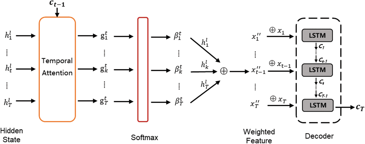
Figure 3: A graphical illustration of the temporal attention module

2.4 LSTM-based Encoder and Decoder

The encoder-decoder is essentially an RNN that encodes the word series into a feature in the machine translation task. The LSTM-based recurrent neural network is used to extract weighted feature series as feature representations in both the factor and temporal attention module. The benefit of an LSTM unit is that the cell state sums activities over time, which can overcome the problem of vanishing gradients and better capture long-term dependencies of time series.

In Fig. 2, it learns the following feature representations from weighted feature series xt′ at time t.

htl=f1(ht−1l,xt′)(10)

where ht∈Rm is the hidden state of the encoder at time step t, m is the size of hidden cells in the encoder, f1 is a LSTM-based non-linear activation function. Thereby, we get the hidden state hl of each time step.

In each LSTM cell, it represents input gate state, ft forget gate state, st cell state, ot output gate and htl the hidden layer output in the current time step. The calculation formula of the LSTM (Encoder) unit is as follows:

ft=σ(Wf[ht−1l;xt′]+bf)(11)

it=σ(Wi[ht−1l;xt′]+bi)(12)

ot=σ(Wo[ht−1l;xt′]+bo)(13)

st=ftst−1+ittanh⁡(Ws[ht−1l;xt′]+bs)(14)

htl=ot⊙tanh⁡(st)(15)

where ht−1l is the previous hidden state of encoder, xt′ is current input, σ is a logistic sigmoid function and ⊙ is a factors-wise multiplication, Wf, Wi, Wo, Ws∈Rm×(m+n) and bf, bi, bo, bs∈Rm.

In the decoder, it can be applied to learn a mapping function f2. Weighting all hidden states hl make it easier to maintain temporal relationships, the result can be used to update the decoder’s hidden state:

ct=f2(ct−1,zt−1)(16)

where ct∈Rm+n is the hidden state of the decoder at time t, f2 is also an LSTM unit. Finally, we take the last hidden state cT as the output of the decoder, which is used to obtain the final prediction through a full-connection layer. The calculation formula is as follows:

y^T=vyTcT+by(17)

where vyT∈Rm+n and by∈R1 are parameters to learn.

3  Experimental Settings

3.1 Datasets and Network Setups

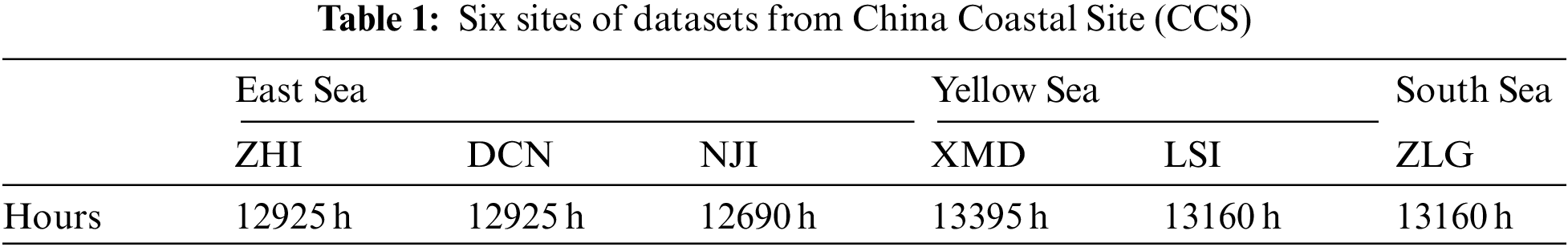
Our datasets come from China Coastal Site (CCS) monitoring data, including multi-factor hydrologic data observed in 13 sites in China seas. As shown in Tab. 1, to demonstrate the generalization ability, we employ six sites of datasets (ZHI, XMD, DCN, LSI, NJI, ZLG where are in East Sea, South Sea and Yellow Sea of China) to verify the proposed methods. The data were sampled every hour from 2012/1 to 2013/7. ZHI and DCN correspond to approximately 12925 h of monitoring data. LSI and ZLG correspond to approximately 13160 h of monitoring data. XMD and NJI correspond to roughly 13395, 12690 h of monitoring data, respectively.

In our experiment, we employed the SST as the prediction factor. The CCS data contains ten ocean environment factors, but they aren’t all necessarily used in our model because some are not associated with SST. Therefore, we selected four relevant factors: air temperature, air pressure, wind speed, and wind direction. To ensure the reliability of the model, we first preprocessed the data. Then, we explained that if some measures were missing, they were replaced by a default value (MISSING_VAL = −999) but for features that are not measures there is still the possibility to get NAN. Thus, we replaced every NAN by the mean value of the five valid values before and after the NAN for features that are not measures.

In our experiment, we roughly divided the training set and the test set at the ratio of 4:1. That is, the first 80% of the datasets are used as training sets and the last 20% as test sets. The proposed model was developed based on a deep learning framework Keras Theano, and used the Adam optimizer. The initial learning rate was set to 0.0001. The experimental environment is Windows10, Intel Core i7 3.0GHZ and 8GB RAM.

3.2 Evaluation Metrics

In this paper, we evaluated the effectiveness of various prediction methods using PACC, RMSE, and the mean absolute error (MAE). They are computed as follows:

RMSE=∑i=1N⁡(yreal,i−ypred,i)2N(18)

PACC=1−∑i=1N⁡(|yreal,i−ypred,iyreal,i|)N(19)

MAE=∑i=1N⁡|yreal,i−ypred,i|N(20)

where yreal,i  is the true SST value of the i−th sample, ypred,i is prediction value of the i−th sample, and N is the total number of the prediction output data. The smaller the values of MAE and RMSE, the better the performance. The value of PACC is positively correlated with the performance of the model. In our experiments, we performed 5-fold cross validation while training.

4  Simulation Results and Analysis

4.1 Comparison of SST Prediction Performance

In order to demonstrate the effectiveness of the TMA-Seq2seq, we compare the current advanced SST prediction methods, such as SVR, LSTM. For these methods, we also use the same multi-factor time series data and parameters for SST prediction. Among them, LSTM-ED is an encoder-decoder network with two layers of LSTM. And we employ the SVR method with linear, polynomial and radial basis function kernel, respectively, and then select the best results, which can realize nonlinear mapping with few parameters.

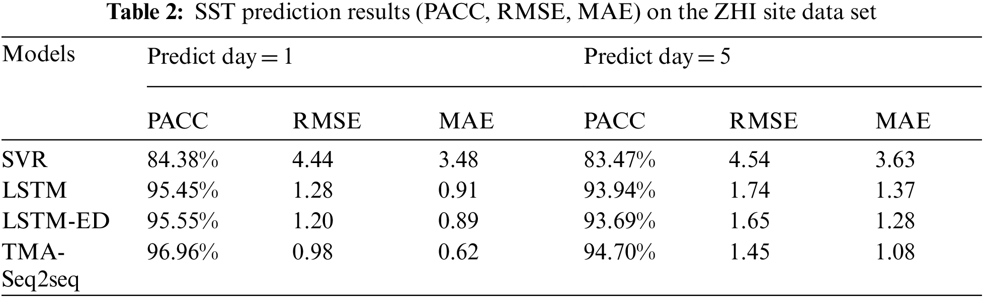
Tab. 2 shows the model performance on the ZHI site data set. PACC of SVR and LSTM are 84.38% and 95.45%, and the RMSE is 4.44 and 1.28 for one day SST prediction. The PACC of LSTM-ED is 95.55%, and the RMSE is 1.20, both of which are better than SVR and LSTM, which further indicates that encoder-decoder also has a certain advantage over LSTM in time series prediction ability. The experimental results show that TMA-Seq2Seq model has the best performance compared with the other three methods. Its PACC, RMSE for one-day prediction are 96.96% and 0.98, respectively, for five-day SST prediction are 94.70% and 1.45.Factor and temporal attention module can learn the influence of historical SST on the predicted SST and the influence of other ocean factors on SST by assigning different attention weights, which makes the model closer to reality and contains more comprehensive information, finally improving the prediction accuracy of SST.

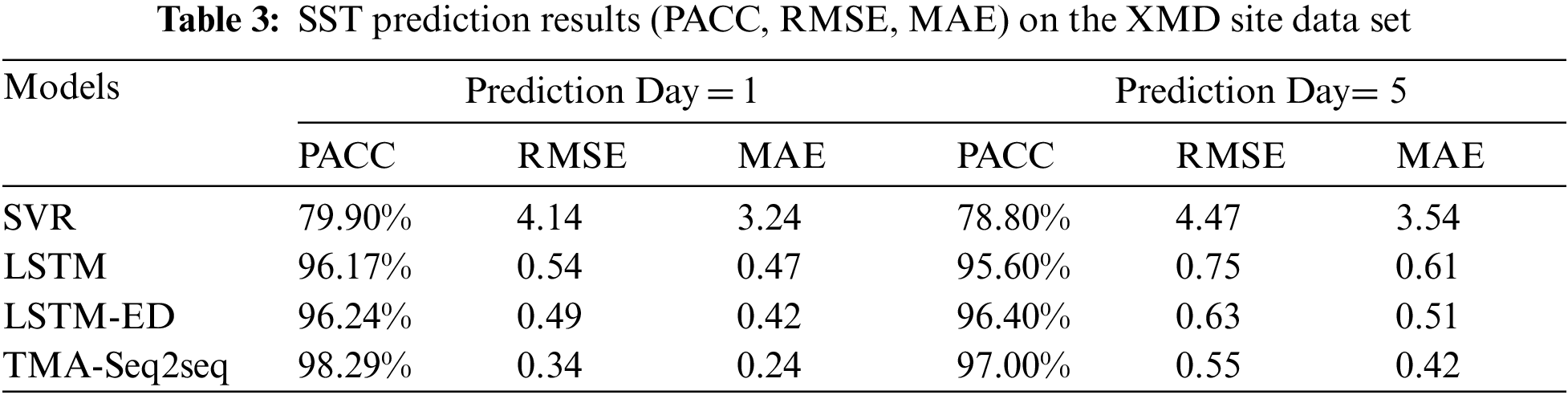
In Tab. 3, we use the XMD site data set to make SST time series prediction, which further verifies the validity of the model and the above conclusions. With the integration of the factor attention module as well as temporal attention module, our proposed model TMA-Seq2seq also achieves the best performance. Its PACC, RMSE reach 98.29%, 0.34 for one-day prediction and 97.00%, 0.55 for five-day prediction. It is notable that the prediction results of TMA-Seq2seq using XMD site data are generally better than that of ZHI site data.

To observe the prediction effect of SST more intuitively, we show the value of 100 moments over the ZHI and XMD testing datasets in Figs. 4a and 4b, respectively. We compare the difference between the real values and prediction values of LSTM and TMA-Seq2seq on the testing data set for 100 days. And the time span of the testing data set is shifted from spring to summer, so both datasets show an upward trend. In Figs. 4a and 4b, the solid red line represents the real value, and the dotted line represents the prediction value of the different methods. And we observe that that generally fits the real values much better than LSTM. In addition, we can find that the XMD site data are more stable than the ZHI, which explains the difference in the accuracy and error of TMA-Seq2seq in the prediction results of Tabs. 2 and 3.

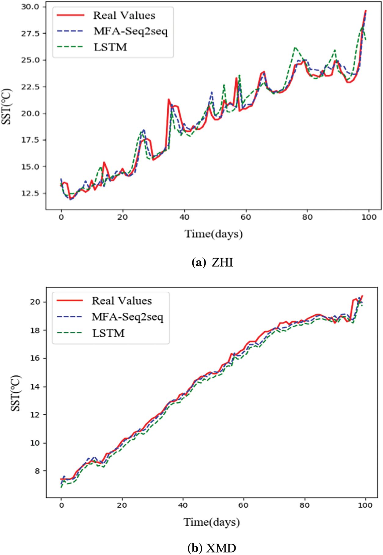
Figure 4: Result of prediction values and real values for LSTM and TMA-Seq2seq. (a) ZHI site data set (b) XMD site data set

In Summary, extensive experiments on the XMD and ZHI site datasets demonstrate that our proposed TMA-Seq2seq model can effectively improve prediction accuracy and both outperform other methods for one day and five-day SST prediction, verifying the validity of the model.

4.2 Impact of Time Window Size

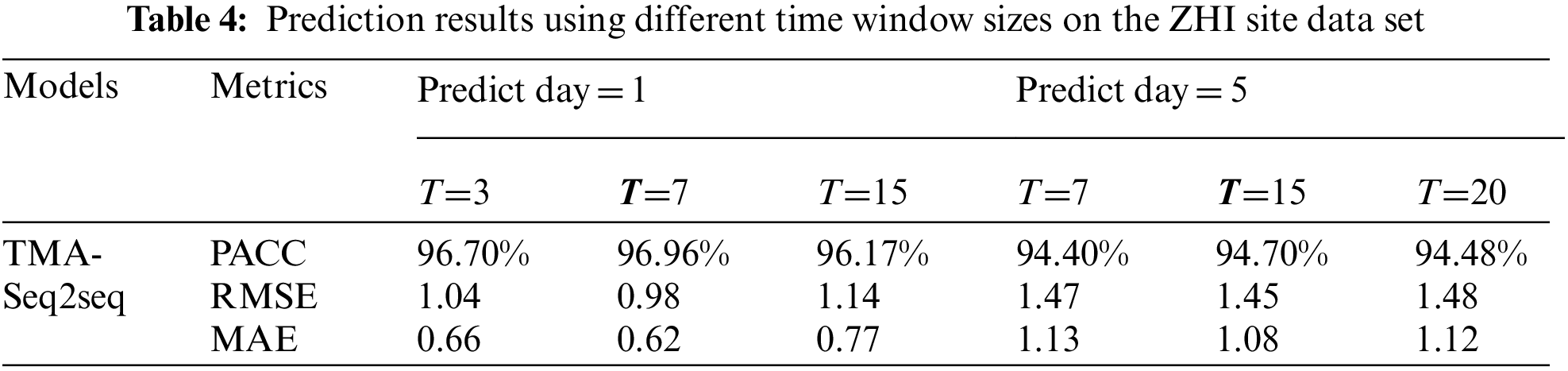
In order to verify the influence of different time window sizes on the SST prediction, we perform experiments according to ZHI site data, using T hours’ historical SST data to predict the future SST, i.e., the future one-day (24 h) and five days (24, 48, 72, 96, 120 h). Here, T represents the number of historical SST. To determine the window size T, we set time window T∈{3, 7, 15} for one-day prediction, T∈{7, 15, 20} for five-day prediction.

As shown in Tab. 4, the experimental results show that the smaller window gets better results for one-day prediction, but the bigger window gets better results for five-day prediction. Therefore, the size of the time window has different impact on the prediction results of the model, so all experiments in this paper use the 7 h’ history SST for the prediction of the future one-day and 15 h’ history SST for the prediction of the future five days.

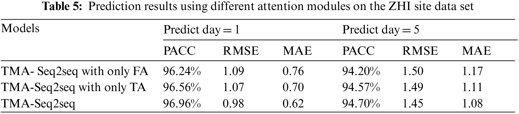
4.3 Effect of Attention Modules

The factor attention and temporal attention can improve the performance of our SST prediction model, as evidenced by an ablation study with the ZHI site data. As shown in Tab. 5, three methods are investigated: the TMA-Seq2Seq model with only factor attention (FA), the TMA-Seq2Seq model with only temporal attention (TA), and the proposed TMA-Seq2Seq method. Firstly, compared with Tab. 2, TMA-Seq2Seq with either factor or temporal attention module can better predict the SST than LSTM and LSTM-ED. Secondly, the TMA-Seq2Seq model with only TA is slightly superior to the TMA-Seq2Seq model with only FA. Nevertheless, TMA-Seq2Seq with both factor and temporal attention module achieves higher accuracy than with single attention module. Therefore, the results show that the Seq2seq model with the integration of the factor attention module and temporal attention module can achieves higher accuracy by extracting the correlation of the multiple factors and the deeper time information.

4.4 Effects of Multi-Factor

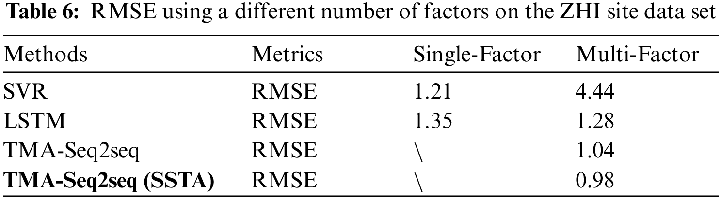
To further illustrate the potential effects of the multiple factors for SST prediction, we compare the results of different methods (SVR, LSTM, TMA-Seq2seq) using single-factor and multi-factor time series data. The results are shown in Tab. 6. The single-factor uses only SST time series data to predict future SST, and multi-factor time series data includes SST, air temperature, air pressure, wind speed, wind direction, SST and SSTA. As shown in Tab. 6, we find that SVR has poor prediction performance when using multi-factor time series data. However, LSTM has a better effect when using multiple factors, but the improvement effect is not significant because there is no module selected in the network. TMA-Seq2seq is our proposed model and its RMSE achieves lower than other methods. In addition, to further show the influence of SSTA, we add the new factor SSTA to input data to predict SST, and the results show that SSTA is beneficial to further lower RMSE. Overall, multi-factor time series data have an obvious influence on the SST prediction error.

To further investigate the factor attention mechanism, we plot the factor attention weights of TMA-Ses2seq for the six factors on ZHI training set and testing set in Fig. 5. The attention weights in Fig. 5 are taken from a single time window, and similar patterns can also be observed for other time windows. We find that the factor attention mechanism in the training set can automatically assign larger weights to the four factors (air temperature, wind speed, SST and SST Anomaly) and smaller weights to the two factors series (wind direction, air pressure) using the activation of the factor attention network to scale these weights. The assignment of factor attention weight is more evident in the testing set. The factor attention mechanism assigns more significant weight to wind speed and air temperature, which is consistent with the existing research results based on correlation analysis. This further illustrates the effectiveness of our proposed factor attention mechanism.

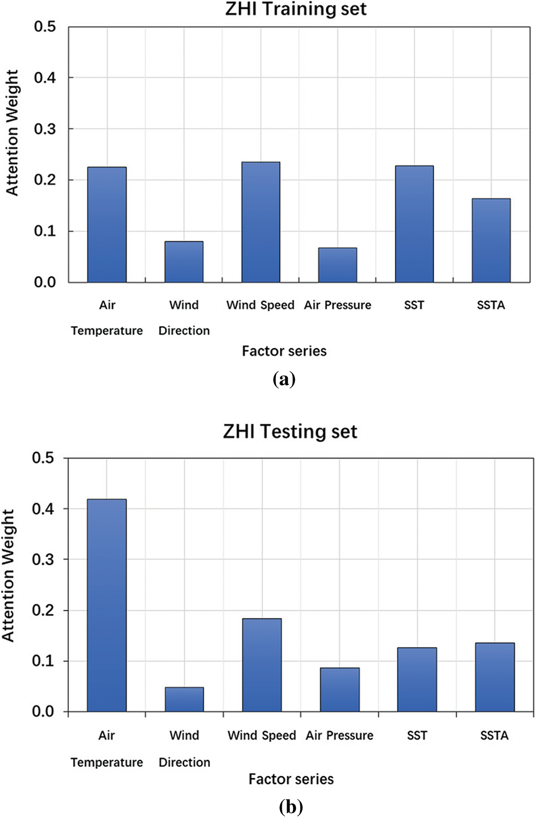
Figure 5: The distribution of the factor attention weights for TMA-Seq2seq from a single time window. (a) ZHI training set (b) ZHI testing set

In summary, the experiment results demonstrates that multi-factor time series can effectively improve the SST prediction accuracy and SST anomaly is helpful to some extent. And the visualization of attention weight enables us to observe the correlation between different ocean environment factors and SST more intuitively, making the network interpretable.

4.5 Robustness of the Model

In order to verify the robustness and generalization of our proposed multi-factor prediction model, we further used the data from different sites to conduct experiments. The datasets were collected from six zones of the China Coastal Site (CCS), denoted by ZHI, XMD, DCN, LSI, NJI, ZLG. The ZHI, DCN and NJI are located in the East China Sea, XMD and LSI are located in the Yellow China Sea, ZLG is located in the South China Sea. Two training strategies were adopted. The first is that we only use single site’s data in the East China Sea to train the model and test the model performance for the other five sites in China’s East, South and Yellow Sea. The second is that we use 80% of the data from all six sites to train the model and test the model for all the site’s data. The results are shown in Tabs. 7 and 8 for the two strategies, respectively. And the models used by these two strategies do not consider the original input characteristics. Finally, we consider the original feature and discuss its influence on improving the applicability of the model.

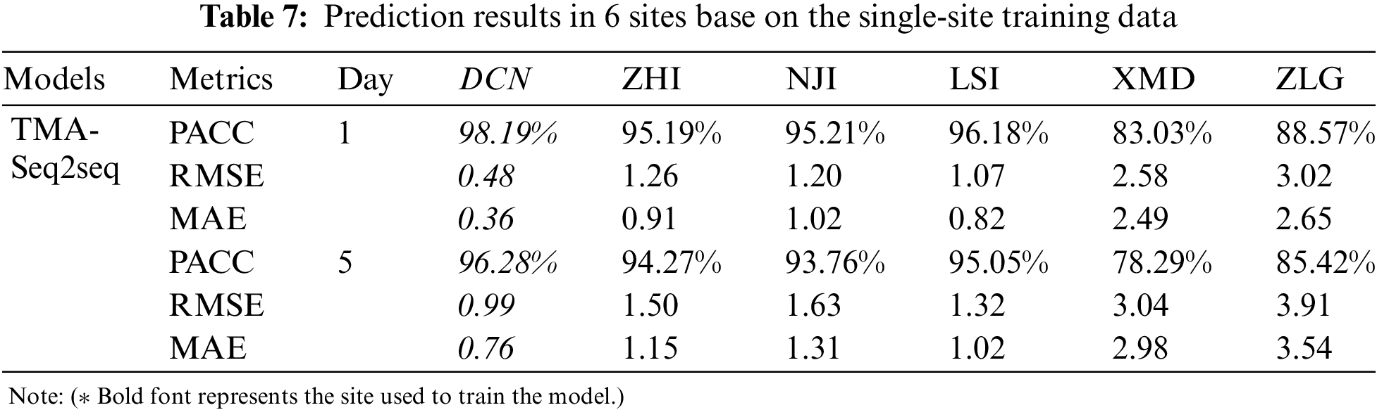
In Tab. 7, the model was trained with 80% of the data from the DCN site and tested with 20% data from the DCN, ZHI, XMD, LSI, NJI, and ZLG to predict the future SST for one day and five days, respectively. The evaluation results show that the sites near to DCN (ZHI, LSI, NJI) get higher prediction accuracy than the sites far away (e.g., XMD in the Yellow Sea and ZLG in the South Sea), whereby the distance between the two sites are calculated by latitude and longitude. The distances of DCN from ZHI, NJI and LSI are 156, 136 and 401 km respectively, and the distances from XMD and ZLG are 845 and 902 km respectively. Therefore, we conclude that the training model may not be suitable for the South China Sea site data, due to the different features of the data at various sea sites.

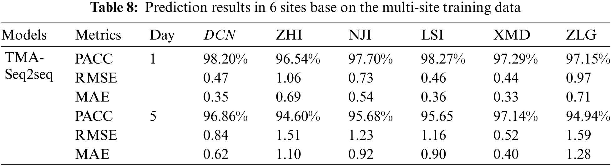
The above experiments show that the model trained by single-site data has limitations when predicting SST in other sea areas. Therefore, we consider the second training strategy. In Tab. 8, the model was trained with 80% of the data from all six sites and tested with 20% data from them to predict the future SST for one day and five days, respectively. Compared with the first training strategy, the evaluation results show that using the data from all the six sites gets higher prediction accuracy and lower error. For one-day SST prediction, accuracy results are higher than 96.54% for one-day prediction and 94.60% for five-day SST prediction. Therefore, we conclude that the model trained with multi-site data can effectively improve this problem.

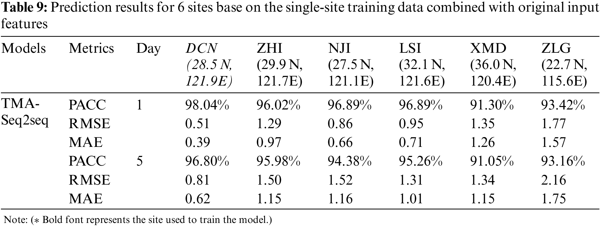
In addition, we also consider whether the model can improve the accuracy of multi-site prediction by enriching features. Therefore, we design the fusion of the original sequence as feature vector and the time-attention-weighted feature as the input of the decoder for SST prediction. The purpose is to enable the model to preserve the low-level distribution feature of the data. The experimental results are shown in Tab. 9, the test results of the model trained with DCN site data are compared with Tab. 7,XMD for five-day SST prediction accuracy increased by 12.16% and RMSE decreased by 1.83. Compared with Tab. 8, the accuracy gap of multi-site prediction results is significantly reduced. It is a very effective method when multi-site history data is not unavailable. The prediction accuracy of our proposed model has strong applicability and robustness.

5  Conclusion and Future Work

In this paper, we proposed a two-module attention-based sequence-to-sequence network (TMA-Seq2seq) for long-term time series SST prediction, which significantly improves the prediction accuracy. We achieved this goal using a two-module: factor-attention and temporal-attention modules and the input of multi-factor time series. The newly introduced factor attention module can adaptively select the relevant factor feature. The temporal attention module can naturally capture the long-term temporal information of the encoded feature representations. Based upon these two attention mechanisms, the TMA-Seq2seq can not only adaptively select the most relevant factor features but can also capture the long-term temporal dependencies of a time series SST data appropriately. Extensive experiments on China Coastal Sites (CCS) demonstrated that our proposed TMA-Seq2seq model can outperform other methods for SST time series prediction. In addition, experiments on different sea sites prove that our model has practical value in SST prediction and has strong robustness.

According to this study, adding the processed factor of SSTA has improved the SST prediction accuracy. In the future, it is worth studying how to comprehensively consider the influence of ocean environmental physical mechanism and spatial dimension on sea surface temperature.

Funding Statement: This study was funded by the work is supported by the National Key R&D Program of China (2016YFC1401903), the Program for the Capacity Development of Shanghai Local Colleges No.20050501900, Shanghai Education Development Fund Project (Grant NO. AASH2004). This work was funded by the Researchers Supporting Project No. (RSP2022R509) King Saud University, Riyadh, Saudi Arabia.

Conflicts of Interest: The authors declare that they have no conflicts of interest to report regarding the present study.

This work is licensed under a Creative Commons Attribution 4.0 International License, which permits unrestricted use, distribution, and reproduction in any medium, provided the original work is properly cited.