Computers, Materials & Continua DOI:10.32604/cmc.2022.027064
Article

Vertex Cover Optimization Using a Novel Graph Decomposition Approach

Abdul Manan1, Shahida Bashir1 and Abdul Majid2,*

1Department of Mathematics, University of Gujrat, Gujrat, 50700, Pakistan
2Department of Physics, University of Gujrat, Gujrat, 50700, Pakistan
*Corresponding Author: Abdul Majid. Email: abdulmajid40@uog.edu.pk
Received: 10 January 2022; Accepted: 30 March 2022

Abstract: The minimum vertex cover problem (MVCP) is a well-known combinatorial optimization problem of graph theory. The MVCP is an NP (nondeterministic polynomial) complete problem and it has an exponential growing complexity with respect to the size of a graph. No algorithm exits till date that can exactly solve the problem in a deterministic polynomial time scale. However, several algorithms are proposed that solve the problem approximately in a short polynomial time scale. Such algorithms are useful for large size graphs, for which exact solution of MVCP is impossible with current computational resources. The MVCP has a wide range of applications in the fields like bioinformatics, biochemistry, circuit design, electrical engineering, data aggregation, networking, internet traffic monitoring, pattern recognition, marketing and franchising etc. This work aims to solve the MVCP approximately by a novel graph decomposition approach. The decomposition of the graph yields a subgraph that contains edges shared by triangular edge structures. A subgraph is covered to yield a subgraph that forms one or more Hamiltonian cycles or paths. In order to reduce complexity of the algorithm a new strategy is also proposed. The reduction strategy can be used for any algorithm solving MVCP. Based on the graph decomposition and the reduction strategy, two algorithms are formulated to approximately solve the MVCP. These algorithms are tested using well known standard benchmark graphs. The key feature of the results is a good approximate error ratio and improvement in optimum vertex cover values for few graphs.

Keywords: Combinatorial optimization; graph theory; minimum vertex cover problem; maximum independent set; maximum degree greedy approach; approximation algorithms; benchmark instances

1  Introduction

The Minimum Vertex Cover Problem (MVCP) is a subset of NP complete problems. Solution of NP class of problems is one of the seven outstanding millennium problems stated by the Clay Mathematics institute. The solution of these problems can be verified in polynomial time scale, but time complexity for solving these problems grow exponentially with size of the problems [1]. The MVCP involves finding a set U such thatU⊂V. Here the set U has the smallest possible cardinality in a graph G=G(V,E) such that V is a set of vertices and E is a set of edges of the graph. For the set U to be a cover of graph, every edge of the graph is connected to at least one element ofU. The set U is called a minimum vertex cover of G [2]. The problem has an exponentially growing complexity since the number of combinations which are required to be verified grows as nv! where nv represents the number of vertices in the graph. Due to exponential growth in complexity of the problem, it is almost impossible to exactly solve the problem in a realistic time scale. Therefore, solving these problems via Brute force method i.e., checking all the possible combinations is not feasible. However, one may opt for an approximate solution of these problems in a reasonably quick time.

The MVCP has a wide range of applications; for example, cyber security, setting up or dismantling of a network, circuit design, biochemistry, bioinformatics, electrical engineering, data aggregation, immunization strategies in network, network security, internet traffic monitoring, wireless network design, network source location problem, marketing and franchising, pattern recognition and cellular phone networking [3–9].

Due to its wide range of applications, the MVCP has received special attention in the scientific community. Several approximate algorithms for solving the problem have been proposed, e.g., the depth first search algorithm, the maximum degree greedy algorithm, the edge weighting algorithm, the deterministic distributed algorithm, the genetic algorithm, the edge deletion algorithm, the support ratio algorithm, the list left algorithm, the list right algorithm and iterated local search algorithm etc [10]. Since all these algorithms provide approximate results with certain accuracy, there is a certain space to improve accuracy and to reduce complexity by introducing faster and more accurate algorithms. The scientific community around the globe has proposed approximate solutions of the problem with polynomial complexity. Some of the efforts by scientific community are described in following paragraph.

Jiaki Gu et al. proposed an algorithm that uses a general three stage strategy to solve the minimum vertex cover problem. Their method includes graph reduction, finding minimum vertex cover of bipartite graph components and finally finding the vertex cover of actual graph [11]. Changsheng Quan and coworkers proposed an edge waiting algorithm to solve MVCP. They claim that their algorithm has a fast-searching performance for solving large-scale real-world problem [12]. Shaowei Cai et al. in their work proposed a heuristic algorithm that make use of a preprocessing algorithm, construction algorithms and search algorithms to solve the MVCP. They claim that their algorithm is fast and accurate as compared to other existing heuristic algorithms [13]. Chuan Luo et al. proposed an algorithm that uses a highly parametric framework and incorporates many effective local search techniques to solve the MVCP. According to their claim their algorithm performs better for medium size graph and is competitive for large sized graphs [14].

Jinkun Chen and coworkers proposed an approximate algorithm based on rough sets. They use a Boolean function with conjunction and disjunction logics [15]. Cai. S et al. in their work use an edge weighting local search technique for finding an approximate MVC [16]. Khan, I and coworkers proposed an algorithm that works by removal of nodes to find a maximum independent set yielding an approximate MVC [17]. Arstrand, M et al. formulated a deterministic distributed algorithm to solve the MVCP. The authors solved the problem for two approximate solutions of the MVC during (Δ+1)2 synchronous communication rounds where Δ represents an upper bound of maximum degree [18]. Bar-Yehuda et al. used Dijkstra algorithm in their work in order to solve the problem [19]. Genetic algorithm has been used for the solution of the problem by Bhasin et al. Their algorithm demonstrated advantage of handling graphs when compared to the reported literature algorithms. The authors mentioned that the algorithm is unable to tackle some problems due to which they proposed the usage of Diploid Genetic Algorithms as an extension [20]. Support Ratio Algorithm (SRA) used a heuristic approach to solve the MVCP in which Balaji and coworkers used an adjacency binary matrix to represent a graph. The complexity of the algorithm has been O(nenv2), where ne is number of edges and nv is the number of vertices. The authors claim that the support ratio algorithm has been found better for large scale problems compared to the reported algorithms [21]. Kettani and co-workers introduced a novel heuristic algorithm to find MVC. The author suggested to use their algorithm for other graph optimization problems including maximum clique problem [22]. Xu and Kumar proposed a solver for the minimum weighted vertex cover problem (MWVC). Their algorithm reformulated a series of SAT (satisfiability) instances using a primal-dual approximation algorithm as a starting point [23]. Ruizhi Li, and coworkers proposed a local search algorithm with tabu strategy and perturbation mechanism for generalized vertex cover problem [24]. For hypergraphs and bounded degree graphs Halperin and co-workers proposed an algorithm to find minimum vertex. They used semi-definite programing and introduced a new rounding technique for this purpose [25]. Cai, S. et al. have reported an algorithm based on local search (NuMVC) that has been found efficient in finding MVC. They introduced two new processes that involve a two-way exchange and an edge weighting mechanism [26].

The literature survey indicates variety of results as far as complexity and accuracy of algorithms are concerned. Onak and Rubinfeld developed a randomized algorithm for maintaining an approximate maximum cardinality matching with a time complexity of O(log2nv) [27].

In particular, the present work is more suitable for two dimensional graphs with triangular grid structures. The two-dimensional triangular grid graphs are very common in telecommunications, in molecular biology, in configurational statistics of polymers and in various other fields [28–30]. We are proposing here a new way to find edges shared by such triangular grid structures and use these subgraphs to simplify the MVC for such graphs.

2  Definitions

A graph can be represented as a matrix Me (Edge Matrix or Adjacency Matrix) such that;

Me=[eij],whereeij={1if(i,j)∈E0if(i,j)∉E

Herei and j are numbered vertices such thati,j∈V.

The setN(k) is the set of neighbors of the kth vertex in the graph. The set of edges connected by the kth vertex is represented by kth row or kth column of the edge matrix. The removal of the kth row and kth column from the edge matrix Me is equivalent to the removal of the kth vertex and all of its incident edges from the graph.

From here onward let HO denote a Hamiltonian cycle with odd number of edges (subgraphs of the form triangles, pentagons and heptagons etc.), HT denote a Hamiltonian cycle with three edges (triangles only), a common or shared edge here is defined as an edge that is shared by more than one Hamiltonian cycles of the form HO. A Hamiltonian cycle with three edges i.e., HT can be represented aseijejkeki=1, where i,j and k are the three vertices of that Hamiltonian cycle. Similarly, for any odd number of vertices i,j,k,l…z one can represent the Hamiltonian cycle HO aseijejkekl…ezi=1.

Any vertex w∈Vc is said to be covered, Vc denotes here the vertex cover of a graph. A∖B implies all those elements of a set A which are not elements of set B and a shared vertex is defined here as a vertex that has a degree greater than two.

3  Proposed Work

A graph can be divided into a number of subgraphs such that;

G(V,E)=⋃i=1rGi(Vi,Ei)(1)

One may construct these subgraphsGi’s such thatEi∩⁡Ej=∅, that is these subgraphs do not share any edge. Yet, there are two possibilities, Vi∩Vj=∅ or Vi∩Vj≠∅ fori,j∈{1,2,3,…,r}. If Vi∩Vj=∅,(i,j=1,2,3,…,r), C=⋃i=1rCi is minimum vertex cover of G, where Ci is the minimum vertex cover ofGi. But if Vi∩Vj≠∅, a union of the intersections of each such pair will yield a set of vertices that may not be covered by individual subgraphs. In that case C does not represents the minimum vertex cover of the graph G. However, the union does not necessarily require to be union of intersection of all the pairs, rather union of intersection of fewer pairs may yield an optimum solution. Let us denote the optimum union set as U. Covering all vertices of U and removing from the graph G will leaveUi∩Gj=∅, i.e., all these subgraphs become disjoint and vertex cover becomesC=U⋃i=1rCi. Let U⊆V be a set with a minimum cardinality among the other sets, exclusion of which assuresGi∩Gj=∅ (where subgraphs Gi and Gj become either isolated paths or Hamiltonian cycles). However, to conveniently decompose a graph into a number of subgraphs and to find the set U is difficult.

A solution for graph decomposition is proposed that is based on Lemma and Theorem proved below.

Lemma: An edge that has both of its vertices covered must belong to a Hamiltonian cycle or a path with odd number of edges.

Proof: A graph can be decomposed into a number of subgraphs that may be a Hamiltonian cycle or a path with odd or even number of edges. For even number of edges a Hamiltonian cycle or path does not require both vertices of any edge to be covered. For a Hamiltonian cycle with odd number of sides only one of the edges must have both vertices covered. For paths with odd number of sides both vertices of one of those edge may or may not require to be covered. Hence, if both vertices of an edge are covered that edge may either be an edge of a Hamiltonian cycle or a path with odd number of edges.

Theorem: The exact minimum vertex cover of a graph Gcan be found by constructing a subgraph from edges (x,y)∈HO and finding minimum vertex cover of the subgraph, where x,y,(x,y)∈G

Proof: For a given set of vertex cover there may exist at most two types of edges depending on the vertices being covered i.e., an edge with both of its vertices covered and an edge with a single vertex covered. The edge with both vertices covered essentially belongs to a subgraph of the form of a path or a Hamiltonian cycle with odd number of edges as proved in the Lemma. In case of two different set of vertex covers i.e., an optimum vertex cover and an approximate one, there can be at most five cases, which are listed below;

Case 1: An edge(x1,y1) covered by both vertices x1andy1 in the set of optimum vertex cover andcovered by a single vertex (either x1ory1) in approximate set of vertex cover.

Case 2: An edge(x2,y2) covered by a single vertex (either x2 or y2) in the optimum set and coveredby both vertices (x2 and y2) in the approximate set.

Case 3: An edge(x3,y3) covered by both vertices x3 and y3 in both sets.

Case 4: An edge(x4,y4) covered by a single but different vertex in both sets.

Case 5: An edge(x5,y5) covered by a single and same vertex in both sets.

For both of the sets the number of cases like case 3, 4 and 5 are the same i.e., such cases do not cause any difference on the cardinality of both sets. In cases 1, 2 and 3 at least one of the sets have its edges covered by both vertices. Since case 3 is the same for both the sets, the only two cases that can cause difference on the cardinality of both sets are case 1 and 2. For the approximate set the number of cases like case 2 is greater than or equal to the number of cases like case 1. This leads to the fact that a large number of cases like case 2 can increase cardinality of an approximate set compared to the optimal set. All edges that belong to subgraphs that are either paths or Hamiltonian cycles with odd number of edges are candidates of having both vertices in the vertex cover. By simply separating all such edges the optimization problem simplifies.

This leads to a conclusion that minimum vertex cover optimization depends only on optimization of subgraphs formed by Hamiltonian cycles or paths with odd number of sides.

Based on the Theorem a new approach is proposed to findu∈U, approximately, and Ci exactly, and hence an approximate minimum vertex cover of the formC=U⋃i=1rCi. In principle, any subgraph of the form HO must have both vertices of one of its edges in the vertex cover. This work is based on finding edges that satisfies eij∈HT. Removal of these edges from the graph assuresEi∩Ej=∅ which is followed by removal of common or shared vertices to result in disjoint graphs satisfying Gi∩Gj=∅.

Our aim here is to find edges, which are common in more than one triangular Hamiltonian cycle. We refer such edges as shared edges. To find such shared edges in a large graph we are proposing a new approach. The new approach is based on decomposition of a graph G(V,E) into two subgraphs GU and GS in such a way that an edge eij∈GS satisfieseij∈HO for at least two subgraphs of the form HO (referred here as shared edges) inG, whereas all edges other than shared edges formsGU. A greedy approach can then be used for selecting a vertex from GS. The selected vertex is then covered. After covering such vertices some of the edges (emn) may no longer satisfy the conditionemn∈HO and hence are moved from GS toGU, the removal of vertices from of GS will eventually result inGS=∅. At this stage the uncovered graphGU will contain shared vertices, isolated polygons and/or isolated paths. This subgraph can further be divided into two subgraphs GI and GSV, where GSV consists of all the shared vertices and their adjacent edges, and GI consists of one or more than one isolated Hamiltonian cycles or paths. Both the subgraphs GSV and GI are covered using maximum degree greedy approach. The greedy approach exactly covers the subgraph GI This work is limited to find subgraph of the form ofHT. i.e., the set of all shared edges of all triangles in a graph. This can be done by finding common neighbors of all edges of the graph. For vertices i and k that form edgeeik, the common neighbors can simply be found by an intersection of a subgraph N(i) with subgraphN(k). The set N(i)∩N(k), is found by carrying out AND operation of ith row or column with kth row or column of the edge matrixMe. One can write; N(i)∩N(k)=eij∧ejk, where j=1,2,3,…,nv and nv is the total number of vertices in the graph. The intersection yields the common neighbors of ith and kth vertices. One can evaluate square of the edge matrix as;

Se=Me2=[∑j=1n⁡eijejk]nv×nv,

An element of matrixSe, i.e., sik=∑j=1n⁡eijejk has the bounds0≤sik≤nv−2, wherei≠k. In matrix Se the diagonal elements sjj(j=1,2,3,…,nv) represent the degree of vertex j, whereas off diagonal elements sik are the number of common neighbors of the vertices i andk, or the number of triangles sharing the edge eik if the edge exits. In other words, each term in a given elementsik corresponds to a Hamiltonian cycle HT i.e., eijejkeki=1. One can also sort Hamiltonian cycles HO with odd number of edges greater than HT by using eijejkekl…ezi=1 condition, where {i,j,k,l…z} is a set of odd number of vertices. However, the current work is limited to find all Hamiltonian cycles of the formHT.There are nv(nv−1) off-diagonal elements ofSe. Since Se is symmetric i.e.,sik=ski, only nv(nv−1)/2 elements of Se are calculated. A maximum of nv(nv−1)/2 subgraphs can be constructed for each possible pair of verticesi andk. Each of these subgraphs consists of set of vertices {i,k,N(i)∩N(k)} and contains 2sik+eik number of edges. However, construction of such subgraphs is beyond the scope of this work, therefore we restrict ourselves to the evaluation of weighted matrixSe only. The subgraphs are completely covered by the verticesi andk. However, depending on the value ofsikthe verticesi andk may or may not be the minimum vertex cover of that subgraph. The matrix Se does not contain any information about common neighbors other than the total number of common neighbors two vertices can have.

An element-by-element multiplication (just corresponding element multiplication of two matrices) of matrix Se with that of the matrix Me results in a matrix Te such that each element tik=eiksikof Te represents number of tringles that share the edgeeik. The elements of matrix Te are classified as;

tik={0N(i)∩⁡N(k)=∅1|N(i)∩⁡N(k)|=1≥2|N(i)∩⁡N(k)|≥2

For example,tik≥2 corresponds to a subgraph which forms two or more than two triangles with a shared edgeeik. For all the cases withtik≥2, the vertices i andk are the minimum vertex cover of the subgraph. Fortik=0, implies either the edge is not shared oreik∉G. Fortik=1, the subgraph forms a single triangle. The valuetik=0, implies thateik∉HT, but eik∈HO may still be possible. A subgraph GS of all edges satisfying eik∈HT can be generated using the weight matrixTe fortik≥2. However, if all the edges of a graph are shared edges, the condition  tik≥2 will produce a graph of shared edges same as the original graph i.e., GS = G. For such graphs one can modify the condition astik≥tmin+n, where tmin is minimum number of triangles sharing a single edge in that graph and n is a small number. This modification will generate a reduced graph of shared edges. A vertex cover of the reduced subgraph GS removes all shared edges of the form eik∈HT fromG. However, the condition eik∈HO may still not be satisfied.

Removal of any subset of vertices from a graph requires removal of the corresponding row or column from the edge matrixMe. This leads to calculation of new square matrixSe. However, instead of calculating Se from scratch, a low-cost solution is proposed here to reduce the simulation time.

Proposition: Se∗ being the square of matrix Me∗ can be calculated fromSe, where Me∗ is the reduced graph after removal of lth row and lth column fromMe.

Proof: Since

Se=[∑j=1n⁡eijejk]nv×nv(1)

Se can be decomposed as

Se=[∑λ=1l−1⁡eiλeλk]nv×nv+[eilelk]n×n+[∑μ=l+1n⁡eiμeμk]nv×nv

where λ=1,2,3,…,l−1 and μ=l+1,l+2,…,nv

LetF=[eilelk]n×n is an nv×nv matrix that can be obtained by multiplying lth column and lth row of the edge matrixMe. One can write;

Se=[∑λ=1l−1⁡eiλeλk]nv×nv+[∑μ=l+1n⁡eiμeμk]nv×nv+F(2)

Let

S´e=[∑j⁡eijejk]nv×nv(3)

where j=1,2,3,…,l−1,l+1,…,nv

Eqs. (2) and (3) yields;

Se=S´e+F(4)

All elements in lth row and lth column from S´e are zeros, therefore, removing lth row and lth column from S´e yields Se∗, which is the required matrix of order(nv−1)×(nv−1).

Se∗=[∑j⁡eijejk](nv−1)×(nv−1)(5)

Reduced matrixSe∗ is multiplied element by element with Me∗ to evaluateTe∗. As previously discussed, the square matrix elements sik is the number of common neighbors of the vertices i andk, the value sik can be used as a weight to select vertices to be covered.

Algorithms

The decomposition of a graph G into GU andGS (The subgraph containing all shared edges of triangular structures) is accomplished by transforming the matrix Te→We such that[We]ij=min(1,[Te]ij) andtik≥2. The algorithm is divided into three stages. In first stage a vertex with highest degree in the subgraphGS is found and covered. The first stage is terminated whenGS=∅. The subgraphGU does not contain any shared edge that belongs to triangular structures but it may still have edges shared by subgraphs of the formHO. In second stage, the vertex with highest degree is found from GU and covered. After covering all the shared vertices of the graph, the graph is left with isolated paths or polygons. In third stage, a vertex with degree 2 is found and covered. The removal of a vertex from G in all three stages may lead to leaves in the residual graph. Therefore, these leaves are removed by covering their adjacent vertex.

The proposed algorithms are described in the following section. Algorithm 1 and Algorithm 2 are abbreviated as ASE and ASER such that ‘A’ stands for Algorithm, ‘SE’ stands for ‘Shared Edges’ and ‘R’ stands for ‘Reduction Strategy’.

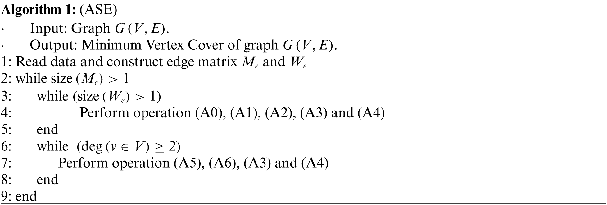
(A0) Evaluate We using matricesMe,Se and Te for tik≥2 or tik≥tmin+3

(A1) Find a vertex with highest degree fromWe and cover the vertex

(A2) Evaluate matrix F for the vertex found in step A1. Using Eq. (4) evaluate reduced matrix Se using matrixF and the matrices Me andSe from step A1. Reduce matrixMe.

(A3) Remove all leaves from the graph

(A4) Remove all isolated vertices from the graph

(A5) Find deg(u∈U), i.e., degree of vertex u in present set of vertices U

(A6) Find the vertex u that has the maximum degree in present graph, cover the selected vertex u and remove from the graph.

Complexity

Total complexity of the algorithm is (34nv3−99nv2+170nv−120)/24≅1.42nv3.

To reduce complexity of ASE a reduction strategy is proposed. The reduction strategy consists of splitting graph into two subgraphs and finding independent set of 1st subgraph and taking union of that independent set with 2nd subgraph and finding independent set of the union set. However, this graph splitting is not random. For splitting one can list the set of edges E={(λ,μ):μ∈N(λ),∀λ,μ∈E}. Construct two sets of vertices L={λ:∀(λ,μ)∈E} andR={μ:∀(λ,μ)∈E}. Find L∩⁡R. One can see that the set, IL=L∖L∩R is an independent set, because there are no two vertices in IL, that are neighbors of each other. Similarly, IR=R∖L∩⁡R is also an independent set.

Under normal circumstances the list of edges E may not provide reasonably large IL and IR, therefore, one may need to prepare the list the edges E so that IL and IR are sufficiently large. One may opt for an alternative strategy to find sufficiently largeIL, IR and a small Vres=L∩R by using a low-cost algorithm that can find an approximate minimum vertex cover. The low-cost algorithm outputs an independent set and residual set of vertices. Therefore, one can use the low-cost algorithm twice to find IL and (V∖IL) and again to find IR and (V∖IL)  ∖IR and remaining set of verticesVres=L∩R. Now one can construct a subgraph fromVres, that is Gres=Gres(Vres,Eres). An independent set Ires can be found using Algorithm 1 (ASE). A second subgraph can be constructed fromIs=IL∪IR∪Ires, that is GS=GS(IS,ES). Using Algorithm ASE again one can construct the final independent set. Complexity of this algorithm depends on the cardinality nL of IL and nR ofIR. The cardinality of set of vertices of the 1st subgraph is n1=nv−nL−nR and cardinality of set of vertices of 2nd subgraph isn2=nres+nL+nR, where nres is the cardinality of the setIres. The complexity of algorithm ASER is[34(n13+n23)−76(n12+n22)+170(n1+n2)−240]/24.

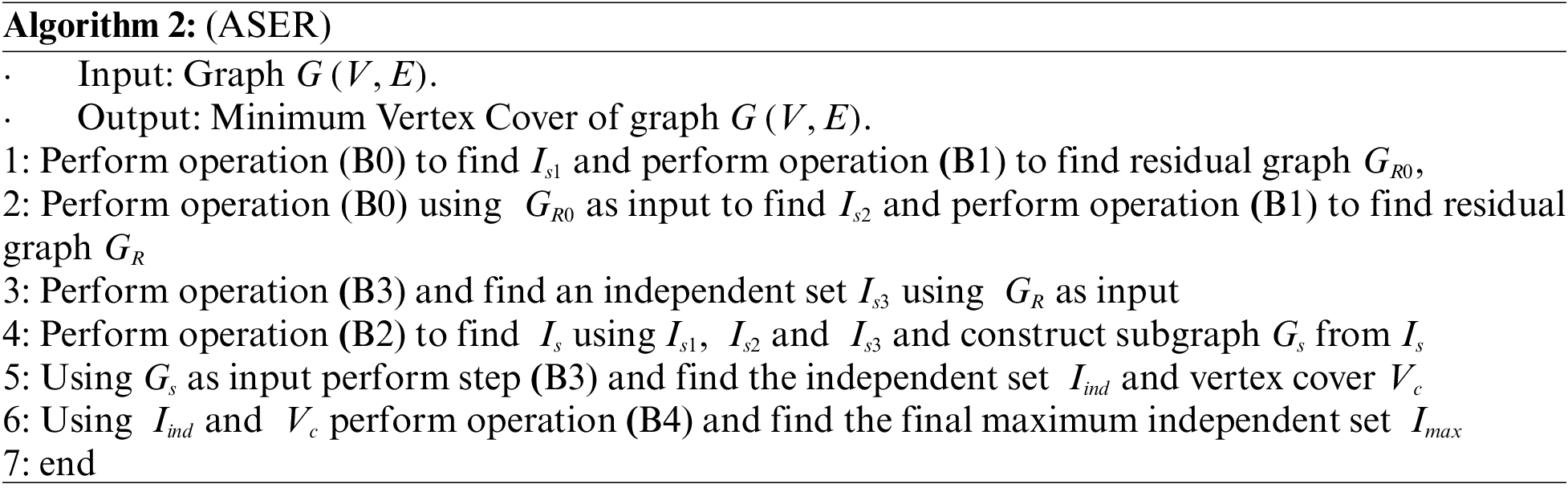
(B0) Find an independent set Is of a graph using a low-cost algorithm

(B1) Construct residual subgraph GR(VR,ER) fromVR=V−Is.

(B2) Construct a single set using three sets as; Is=Is1∪Is2∪Is3

(B3) Find maximum independent set of given subgraphs using algorithm 1

(B4) Find a subset Ic of the vertex coverVc, such that Ic contains vertices that individually can go to independent setIind. Find independent set of Ic using Algorithm1. Move all vertices of that independent set to Iind to construct the final independent set.

The low-cost algorithm simply selects and adds a vertex to an independent set followed by searching vertices that can be moved to the independent set. This algorithm has a complexity ofnv2/2. However, one is free to choose the low-cost algorithm in accordance with the suitability.

4  Results and Discussion

In this section both the algorithms are tested and analyzed for their accuracy and complexity for benchmark graphs taken from [31,32] and [33]. The simulations are performed on a computer with 1.61 GHz processor and 8.00 GB RAM using sequential programming.

The results from the 72 benchmark graphs referred above are organized in the form of three tables. Tabs. 1 and 2 contain optimum vertex cover and accuracy in the form of error ratios for the algorithms of respective graphs. Tab. 3 contains a comparison of results of the algorithm ASE with three well know algorithms. The error ratio is defined here as the value of minimum vertex cover for a given graph obtained from each algorithm divided by the optimum vertex cover(nO) of that graph. The condition  tik≥2 has been used to generate shared edges graph(GS) for 64 benchmark graphs. For some of the benchmark graph all the edges are shared edges, therefore, the condition  tik≥2 will yieldGS=G. For such graphs the condition is modified totik≥tmin+3, where tmin is minimum number of triangles sharing a single edge in that graph. This modification results in reduced shared edges graph. The conditiontik≥tmin+3 is used to generateGS for eight such graphs and their error ratios are given in Tab. 2.

Fig. 1 shows the error ratio (ϵr) obtained from both the algorithms plotted against the number of vertices for 67 benchmark graphs (excluding the graph with number of vertices greater than 2000 for better visibility of the figure). The solid line in Fig. 1 corresponds to the error ratio for optimum vertex cover. It can be seen that the error ratio for graphs with fewer number of vertices is less accurate compared with that of the higher number of vertices. This suggests that the algorithms get better and better with increased number of vertices. It can also be noted that the worst-case error ratio (ϵr) for algorithms ASE and ASER are 1.025 and 1.038 respectively. An interesting finding of this study is the reported optimum error ratio for few benchmark graphs in literature is found slightly less accurate compared to the value calculated in this work. This can be seen in Fig. 1 as ASE and ASER lies below the optimum error ratio line on six and three occasions, respectively.

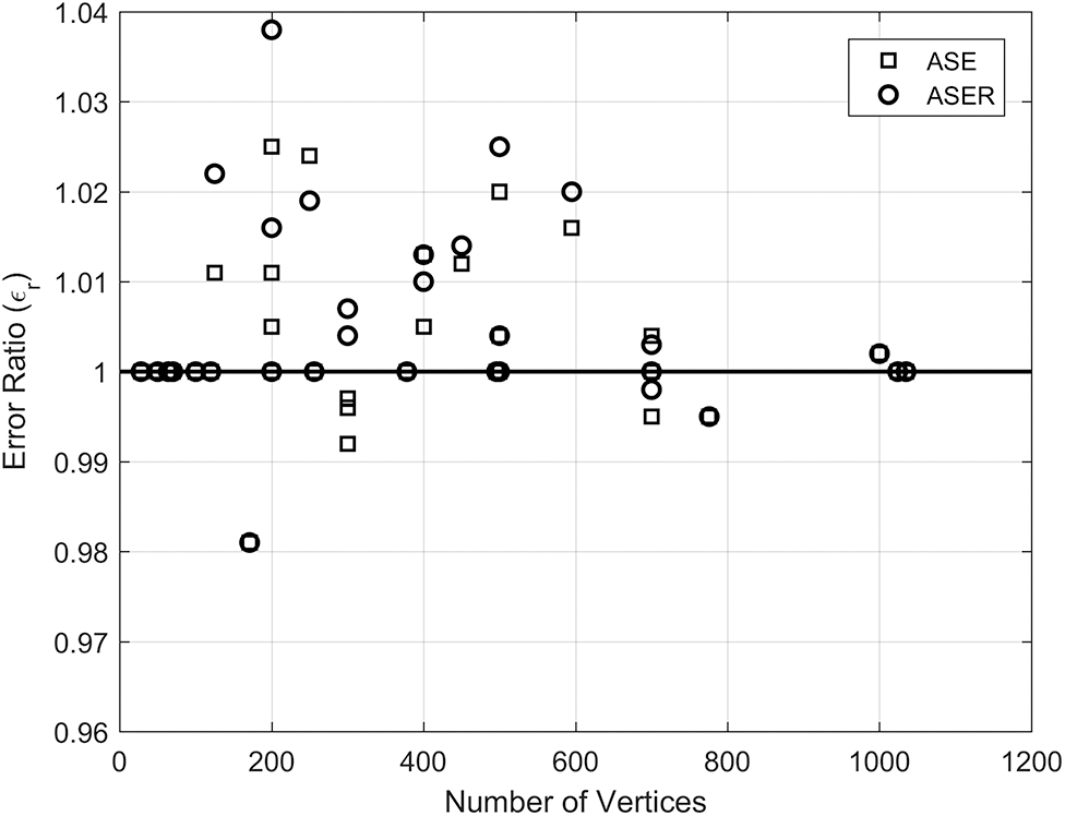
Figure 1: Accuracy of the suggested algorithms, solid line represents reported optimum values

As can be seen from the Tabs. 1 and 2 that out of 72 instances ASE and ASER both give an error ratio (ϵr=1) or better on 55 and 50 instances, respectively. The average error ratios (ϵr) for ASE and ASER are 1.0017 and 1.0030 respectively.

In ASE, since only edgesemn∈HT are covered, all edges satisfying emn∈HO are not covered with certainty. This may lead to erroneous results. After covering all edges from subgraphs of the formHT, shared vertices are selected with the priority of highest degree of the residual graph, and the vertices are moved to vertex cover one by one. The selection may not be accurate since it uses the greedy approach. However, the approach will produce exact minimum vertex cover for the residual graph that is left with isolated Hamiltonian cycles or paths.

Supplementary data describes the complexity of the proposed algorithms and contains two parametric numbers or reduction parameters p1 andp2. Supplementary data also contains time taken by each of the algorithm to find the minimum vertex cover. The reduction parameter is the ratio of approximate complexity of the form (≅1.41n1,23) of an algorithm with that of(≅1.41nv3), and can be is calculated asp1,2=n1,23/nv3, where n1 and n2 are defined in the previous section. These reduction parameters represent a time reduction of an algorithm with reduction strategy (ASER) to the same without reduction strategy (ASE).

The comparison between ASE and ASER is given in Fig. 2, which shows that if either p1→1 orp2→1, a difference between their simulation times approaches to zero. For graphs hamming6_2_clq_compliment, hamming8_2_clq_compliment and hamming10_2_clq_compliment, one can see that p1→1 andp2→0, hence no significant time difference is observed. Similarly, for graphs p_hat700_1, MANN_a27, MANN_a45 and C2000_9 reduction parameters p1→0 andp2→1, forcing the time difference to approach to zero. A noticeable difference in simulation time can be observed for the cases where neither p1→1 nor p2→1. The reduction parameters p1 and p2 for each of the benchmark graphs are plotted in Fig. 2.

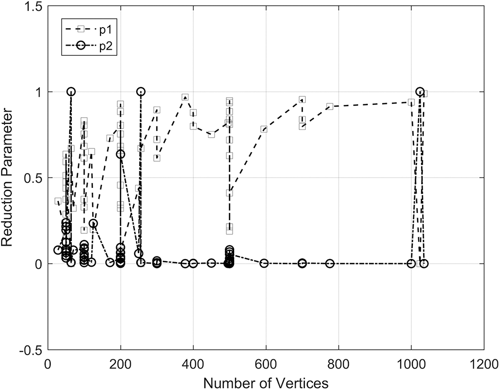
Figure 2: Reduction parameters p1 and p2 plotted against number of vertices

The simulation time for the proposed algorithms is plotted against the number of vertices in Fig. 3. A cubic fit function of the form f(nv)=Cnv3 is also plotted to show the complexity trend of both the algorithms. It can be seen that the algorithms (ASE and ASER) follow the cubic fit trend. Since computer takes a small amount of preprocessing time before each simulation, one can see that for low values ofnv the simulation time is large compared to f(nv), whereas for large values ofnv the simulation time matches withf(nv). One can also see that simulation time for ASER is occasionally smaller thanf(nv), reflecting a success in reduction strategy.

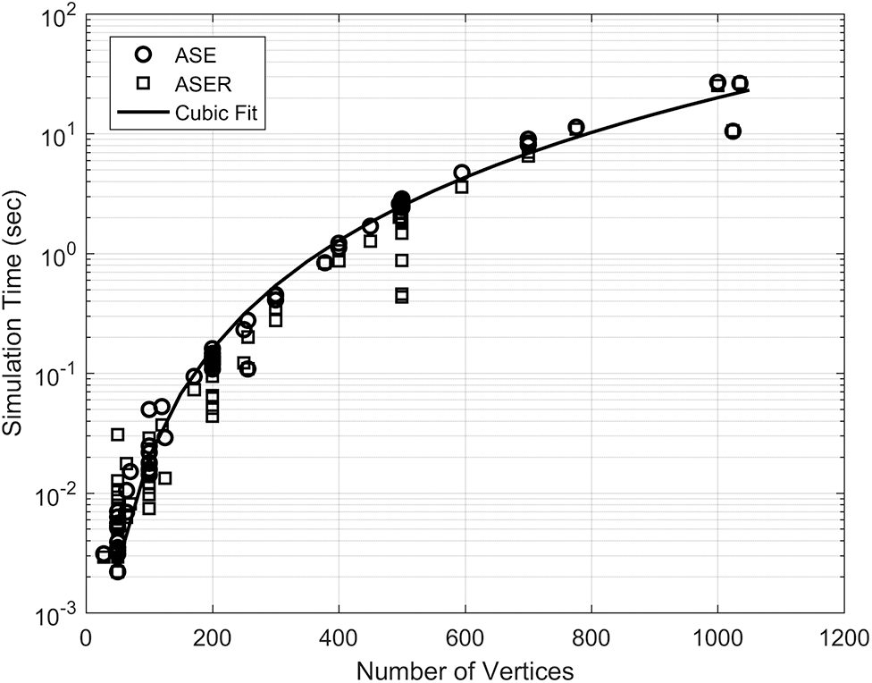
Figure 3: Simulation time vs. the number of vertices for the proposed algorithms

In Tabs. 1 and 2 the performance of the algorithm ASE is evaluated using 72 benchmark graphs. On 48 instances our algorithms yield optimal values. In Tab. 3 we have compared the results for 20 benchmark graphs for which ASE does not yield optimal values with three well known algorithms MDG (maximum degree greedy) [34], MVSA (modified vertex support algorithm) [35] and MtM (Min-to-Min) [36]. The average ratio error for these 20 benchmark graphs presented in the Tab. 3 for ASE, MDG, MVSA and MtM are, 1.005, 1.014, 1.015 and 1.012, respectively. This shows that the algorithm ASE clearly outperforms the three algorithms in comparison.

5  Practical Implementation

For step-by-step analysis of the algorithm a simple real-life example is selected. Crypto or digital currency market currently has a market capital of billions of US dollars. There are hundreds of crypto currencies with billions of USD daily volume. Market data analysis of these currencies is becoming harder and harder with growth in data. However, almost all of these currencies are paired with each other for trading. Therefore, any market fluctuation is coupled within these crypto currencies. In principle, one can represent these currencies and their trading pairs in the form of a graph and can find minimum vertex cover of the graph to select only few currencies for crypto market data analysis. We have selected ten crypto currencies and their trading pairs in order to simplify the problem. These crypto currencies and their trading pair are presented in the form of a graph is shown in Fig. 4a.

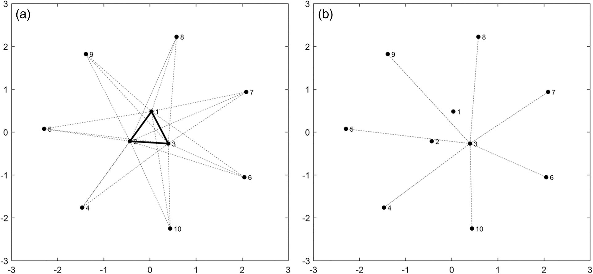
Figure 4: (a) Crypto currencies and their trading pair (b) Subgraph with no shared edge

The graph is decomposed in subgraphs with bold dark lines showing shared edges and dashed lines as the rest of the graph. The shared edge graph is simply a triangle in this case and each vertex has a degree 2 in the subgraph. A single vertex (in this case vertex 1) is covered, i.e., Vc={1} and we are left with only a single edge (e23) in the subgraph. One vertex (vertex 2) of the remaining edge (e23) is covered, yielding Vc={1,2}. Since there are no more shared edges in the graph, therefore we are left with the subgraph of the form shown in Fig. 4b. From here on ward the vertices are simply covered on the basis of their degree. Since the vertex 3 has the highest degree therefore, it is covered, yielding Vc={1,2,3} and hence the entire graph is covered. A conclusion of this process is that, only crypto currencies numbered 1, 2 and 3 represent the complete variation of the market for only these ten crypto currencies. However, in order to completely analyses the entire crypto market a minimum vertex cover of a graph representing entire market has to be found.

6  Summary

The proposed approach simplifies a graph to isolated paths or polygons (Hamiltonian cycles) by moving shared edges followed by shared vertices to the vertex cover. This process forms three subgraphs i.e., a subgraph containing shared edges, a subgraph with shared vertices and finally a simplified subgraph. The final simplified subgraph is either a single Hamilton cycle or path or a number of isolated Hamiltonian cycles or paths. The vertex cover of the simplified subgraph can be exactly found in a short time using maximum degree greedy approach. The accuracy of finding the first two subgraphs depends on the sequence of covering the vertices. The proposed strategies are capable to search for the sequence of selection of vertices to an approximate extent only. However, using this approach the problem can be broken successfully into three smaller problems, which are relatively easy to handle. The worst-case error ratio (ϵr) for algorithms ASE and ASER are 1.025 and 1.038, respectively. The average error ratios (ϵr) for ASE and ASER are 1.0017 and 1.0030 respectively. The algorithms have a maximum complexity of approximately 1.42nv3. Both the algorithms (ASE and ASER) improve optimum error ratio for few graphs compared to the values reported in literature [17,34–36].

7  Future Work

The proposed approach may work even better if all the edges shared by subgraphs of the form HO can be found and removed with certainty (i.e., in correct sequence) and if one may find a better strategy (or sequence) to remove shared vertices other than the greedy approach. A future work is suggested to find shared edges among all subgraphs of the formHO.

Funding Statement: The authors received no specific funding for this study.

Conflicts of Interest: The authors declare that they have no conflicts of interest to report regarding the present study.

References

 1.  S. Cook, “The complexity of theorem proving procedure,” Proceedings of the Third Annual ACM Symposium on Theory of Computing, pp. 151–158, 1971. [Google Scholar]

 2.  Z. Ullah, M. Fayaz and S. H. Lee, “An efficient technique for optimality measurement of approximation algorithms,” International Journal of Modern Education & Computer Science, vol. 11, pp. 11, 2019. [Google Scholar]

 3.  L. Wang, S. Hu, M. Li and J. Zhou, “An exact algorithm for minimum vertex cover problem,” Mathematics, vol. 7, no. 7, pp. 603, 2019. [Google Scholar]

 4.  S. R. Balachandar and K. Kannan, “A Meta-heuristic algorithm for vertex covering problem based on gravity,” International Journal of Mathematical and Statistical Sciences, vol. 1, no. 3, pp. 130–136, 2009. [Google Scholar]

 5.  J. Chen and I. A. Kanj, “Constrained minimum vertex cover in bipartite graphs: Complexity and parameterized algorithms,” Journal of Computer and System Sciences, vol. 67, no. 4, pp. 833–847, 2003. [Google Scholar]

 6.  M. Fayaz, S. Arshad, A. S. Shah and A. Shah, “Approximate methods for minimum vertex cover fail to provide optimal results on small graph instances: A review,” International Journal of Control and Automation, vol. 11, no. 2, pp. 135–150, 2018. [Google Scholar]

 7.  Z. Jin-Hua and Z. Hai-Jun, “Statistical physics of hard combinatorial optimization: Vertex cover problem,” Chinese Physics B, vol. 23, no. 7, pp. 078901, 2014. [Google Scholar]

 8.  M. Javad-Kalbasi, K. Dabiri, S. Valaee and A. Sheikholeslami, “Digitally annealed solution for the vertex cover problem with application in cyber security,” in ICASSP 2019–2019 IEEE Int. Conf. on Acoustics, Speech and Signal Processing (ICASSPpp. 2642–2646, 2019. [Google Scholar]

 9.  D. Zhao, S. Yang, X. Han, S. Zhang and Z. Wang, “Dismantling and vertex cover of network through message passing,” IEEE Transactions on Circuits and Systems II: Express Briefs, vol. 67, no. 11, pp. 2732–2736, 2020. [Google Scholar]

10. J. Chen, K. Lei and C. Xiaochuan, “An approximation algorithm for the minimum vertex cover problem,” Procedia Engineering, vol. 137, pp. 180–185, 2016. [Google Scholar]

11. J. Gu and P. Guo, “PEAVC: An improved minimum vertex cover solver for massive sparse graphs,” Engineering Applications of Artificial Intelligence, vol. 104, pp. 104344, 2021. [Google Scholar]

12. C. Quan and P. Guo, “A local search method based on edge age strategy for minimum vertex cover problem in massive graphs,” Expert Systems with Applications, vol. 182, pp. 115185, 2021. [Google Scholar]

13. S. Cai, J. Lin and C. Luo, “Finding a small vertex cover in massive sparse graphs: Construct, local search, and preprocess,” Journal of Artificial Intelligence Research, vol. 59, pp. 463–494, 2017. [Google Scholar]

14. C. Luo, H. H. Hoos, S. Cai, Q. Lin, H. Zhang et al., “Local search with efficient automatic configuration for minimum vertex over,” in IJCAI, Macau, pp. 1297–1304, 2019. [Google Scholar]

15. J. Chen, Y. Lin, J. Li, G. Lin, Z. Ma et al., “A rough set method for the minimum vertex cover problem of graphs,” Applied Soft Computing, vol. 42, pp. 360–367, 2016. [Google Scholar]

16. S. Cai, K. Su and Q. Chen, “EWLS: A new local search for minimum vertex cover,” in Proc. of the AAAI Conf. on Artificial Intelligence, Atlanta, Georgia, USA, vol. 24, no. 1, 2010. [Google Scholar]

17. I. Khan and N. Riaz, “A new and fast approximation algorithm for vertex cover using a maximum independent set (VCUMI),” Operations Research and Decisions, vol. 25, no. 4, pp. 5–18, 2015. [Google Scholar]

18. M. Åstrand, P. Floréen, V. Polishchuk, J. Rybicki, J. Suomela et al., “A local 2-approximation algorithm for the vertex cover problem,” in Int. Symp. on Distributed Computing, Springer, Berlin, Heidelberg, pp. 191–205, 2009. [Google Scholar]

19. R. Bar-Yehuda and S. Even, “A Linear-time approximation algorithm for the weighted vertex cover problem,” Journal of Algorithms, vol. 2, no. 2, pp. 198–203, 1981. [Google Scholar]

20. H. Bhasin and M. Amini, “The applicability of genetic algorithm to vertex cover,” International Journal of Computer Applications, vol. 123, no. 17, pp. 29–34, 2015. [Google Scholar]

21. S. Balaji, V. Swaminathan and K. Kannan, “An effective algorithm for minimum weighted vertex cover problem,” Int. J. Comput. Math. Sci, vol. 4, pp. 34–38, 2010. [Google Scholar]

22. O. Kettani, F. Ramdani and B. Tadili, “A heuristic approach for the vertex cover problem,” International Journal of Computer Applications, vol. 82, no. 4, pp. 9–11, 2013. [Google Scholar]

23. X. Xu and J. Ma, “An efficient simulated annealing algorithm for the minimum vertex cover problem,” Neurocomputing, vol. 69, no. 7–9, pp. 913–916, 2006. [Google Scholar]

24. R. Li, S. Hu, Y. Wang and M. Yin, “A local search algorithm with tabu strategy and perturbation mechanism for generalized vertex cover problem,” Neural Computing and Applications, vol. 28, no. 7, pp. 1775–1785, 2017. [Google Scholar]

25. E. Halperin, “Improved approximation algorithms for the vertex cover problem in graphs and hypergraphs,” SIAM Journal on Computing, vol. 31, no. 5, pp. 1608–1623, 2002. [Google Scholar]

26. S. Cai, K. Su, C. Luo and A. Sattar, “NuMVC: An efficient local search algorithm for minimum vertex cover,” Journal of Artificial Intelligence Research, vol. 46, pp. 687–716, 2013. [Google Scholar]

27. K. Onak and R. Rubinfeld, “Maintaining a large matching and a small vertex cover,” in Proc. of the Forty-Second ACM Symp. on Theory of Computing, New York, USA, pp. 457–464, 2010. [Google Scholar]

28. V. S. Gordon, Y. L. Orlovich and F. Werner, “Hamiltonian properties of triangular grid graphs,” Discrete Mathematics, vol. 308, no. 24, pp. 6166–6188, 2008. [Google Scholar]

29. Y. Orlovich, G. Valery and F. Werner, “Cyclic properties of triangular grid graphs,” IFAC Proceedings, vol. 39, no. 3, pp. 149–154, 2006. [Google Scholar]

30. R. Jothi and J. Mary, “Cyclic structure of triangular grid graphs using SSP,” International Journal of Pure and Applied Mathematics, vol. 109, no. 9, pp. 46–53, 2016. [Google Scholar]

31. CLIQUE Benchmark Instances. Available online: https://github.com. [Google Scholar]

32. Benchmark graphs. Available online: http://networkrepository.com/dimacs.php. [Google Scholar]

33. Benchmark graphs. Available online: Index of/pub/challenge/graph/benchmarks/clique–DIMAC. [Google Scholar]

34. S. Gajurel and R. Bielefeld, “A simple NOVCA: Near optimal vertex cover algorithm,” Procedia Computer Science, vol. 9, pp. 747–753, 2012. [Google Scholar]

35. I. Khan and K. Hasham, “Modified vertex support algorithm: A new approach for approximation of minimum vertex cover,” Research Journal of Computer and Information Technology Sciences ISSN 2320, 6527, vol. 1, no. 6, pp. 1–6, 2013. [Google Scholar]

36. J. Haider and M. Fayaz, “A smart approximation algorithm for minimum vertex cover roblem based on Min-to-min (MtM) strategy,” (IJACSA) International Journal of Advanced Computer Science and Applications, vol. 11, no. 12, pp. 250–259, 2020. [Google Scholar]

This work is licensed under a Creative Commons Attribution 4.0 International License, which permits unrestricted use, distribution, and reproduction in any medium, provided the original work is properly cited.