Computers, Materials & Continua DOI:10.32604/cmc.2022.027106
Article

Optimization of Channel Estimation Using ELMx-based in Massive MIMO

Apinya Innok1, Chittapon Keawin2 and Peerapong Uthansakul2,*

1Telecommunications Engineering, Rajamangala University of Technology Isan, Nakhon Ratchasima, 30000, Thailand
2School of Telecommunication Engineering, Suranaree University of Technology, Nakhon Ratchasima, 30000, Thailand
*Corresponding Author: Peerapong Uthansakul. Email: uthansakul@sut.ac.th
Received: 11 January 2022; Accepted: 30 March 2022

Abstract: In communication channel estimation, the Least Square (LS) technique has long been a widely accepted and commonly used principle. This is because the simple calculation method is compared with other channel estimation methods. The Minimum Mean Squares Error (MMSE), which is developed later, is devised as the next step because the goal is to reduce the error rate in the communication system from the conventional LS technique which still has a higher error rate. These channel estimations are very important to modern communication systems, especially massive MIMO. Evaluating the massive MIMO channel is one of the most researched and debated topics today. This is essential in technology to overcome traditional performance barriers. The better the channel estimation, the more accurate it is. This paper investigated machine learning (ML) for channel estimation. ML channel estimations based on the Extreme Learning Machine (ELMx) group are also implemented. These estimations, known as the ELMx group, include Regularized Extreme Learning Machine (RELM) and Outlier Robust Extreme Learning Machine (ORELM). Then, it was compared with LS and MMSE. The simulation results reveal that the ELMx group outperforms LS and MMSE in channel capacity and bit error rate. Additionally, this paper has proven complexity for verified computational times. The RELM method is less time consuming and has low complexity which is suitable for future use in large MIMO systems.

Keywords: Channel estimation; capacity; ELM; RELM; ORELM

1  Introduction

At present, wireless communication systems are constantly evolving and become one of the most important aspects of life in the field such as medicine, transportation, economy, and society [1,2]. Lots of people are more accessible. Nowadays the generation 5 (5G) has been achieved by providers, for service and support the use of many people [3]. We think about it in terms of massive MIMO systems with a lot of receiving and sending antennas. Massive MIMO has the advantage of being able to send extraordinarily rapid data. Spatial Diversity is the separation of the reception antennas to improve the radio signal’s reliability. Spatial multiplexing, on the other hand, permits numerous distinct data streams to be sent between the transmitter and the receiver. This significantly boosts throughput or capacity. It also enables numerous network users to be served by a single transmitter, thus the name MU-MIMO. Beamforming uses advanced antenna technology to focus a wireless signal in a specific direction researched to increase network speed and capacity rather than transmitting to a large area. Channel estimation can also be utilized as an improvement approach for massive MIMO. The frequently used channel estimation techniques, such as LS and MMSE channel estimation, are both fundamental techniques. The LS and MMSE, on the other hand, have low precision. Because it does not use a noise technique, LS channel estimation has a low computing complexity. The MMSE, on the other hand, includes noise in its calculations [4]. In communication scenarios, large-scale MIMO systems are a multitude of modeled case studies for optimization. Hybrid large-scale MIMO is an interesting scenario for many researchers [5,6]. However, we chose a large MIMO based system to generate simulation results to process machine learning datasets. In recent years, deep learning has made great progress in the field of big data feature learning. By integrating low-level input for big data with significant diversity and veracity, deep learning models can extract high-level features and build hierarchical representations more effectively. Deep learning for channel estimation has been used to solve nonlinear mapping and nonconvex problems [7,8]. Deep learning also has a high rate of convergence and good regression accuracy. The authors proposed deep learning for super-resolution channel estimation and DOA estimation based on massive MIMO systems in their research paper [9]. Moreover, Channel State Information Prediction for 5G Wireless Communications: A Deep Learning Approach is one to optimize in 5G typically and the result show interesting [10]. Although the deep learning technique performs better, it requires more network training time and is more difficult to calculate channel estimation. With the advancement of big data, optimization algorithm and increased computing resources in promoting enhanced ELM, it is now state-of-the-art (SOA) in areas including brain EEG classification [11]. As a result, we propose ELMx, which combines three machine learning algorithms for channel estimation such as ELM, RELM, and ORELM. The hidden layer bias and input weight are generated at random from distributions [12–14]. The ELMx can learn at a faster rate and perform well in regression. It is used to optimize the number of hidden neuron nodes during the training phase. The signal received is used as input. In terms of Mean Square Error (MSE), Bit Error Rate (BER), Channel Capacity, Outage Probability, Computational Time, and Computational Complexity, the simulation results show that channel estimation performs better. The results indicated that the proposed learning framework was comparable to SOA with less training time. which is important for continuous communication in data transmission.

The following is an overview of the paper’s structure. Section 2 describes the content and approach in-depth, including massive MIMO systems, fundamental channel estimate techniques, and offers machine learning for channel estimation, as well as the features of ELMx. The results are then discussed in Section 3. Finally, in Section 4, the paper’s conclusion is presented.

2  Material and Method

As a system model, we built a general communication system focused on massive MIMO to bring the resulting system to compute various results.

2.1 Massive MIMO Systems

First, as illustrated in Fig. 1, we investigate a typical massive MIMO systems. A block diagram is assumed for delivering data from the X (vector of transmitted signals) to the Y (vector of received signals) with MT transmitting antennas and MR receiving antennas.

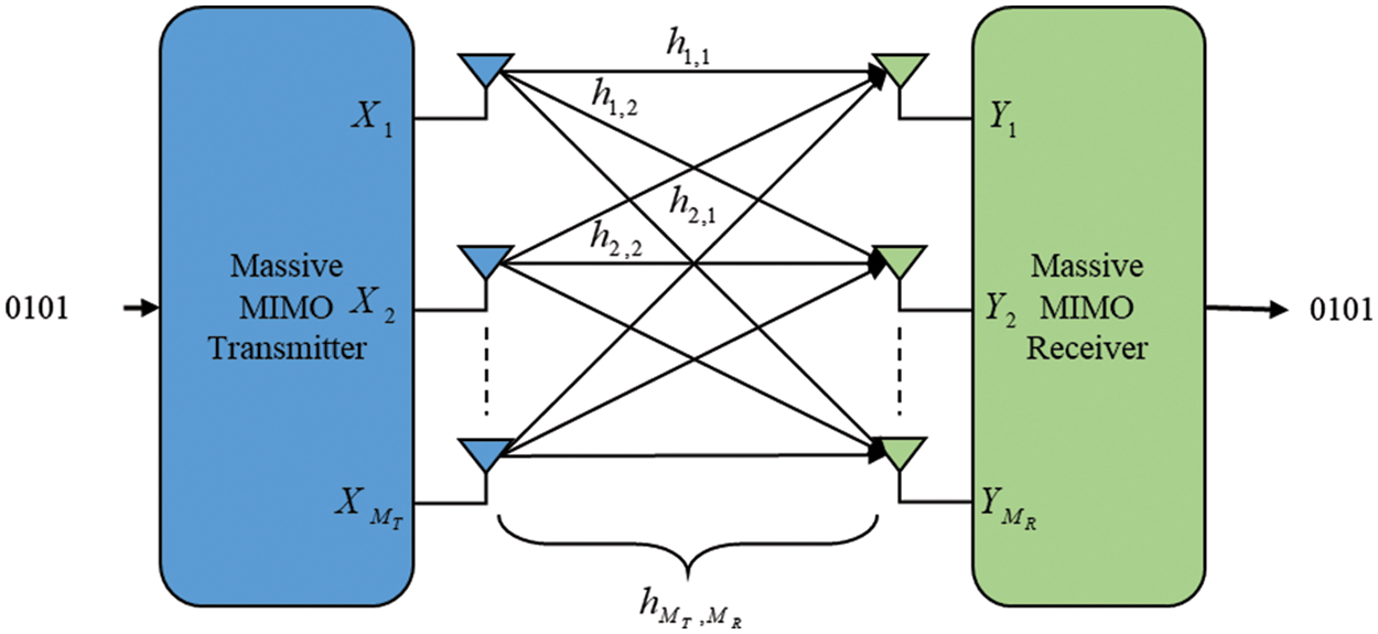
Figure 1: A block diagram of Massive MIMO Systems

The relation between transmitted and received signal is given by

Y=HX+n(1)

where H is a channel response matrix (MR ×MT) and n is an additive white complex Gaussian noise vector (MR × 1) is fundamental noise models used in data theory to mimic the effects of many random processes occurring in nature. The relationship between the transmitted and received signals can be represented by the matrix

[Y1Y2⋮YMR]=[h11h12⋯h1,MTh12h22⋯h2,MT⋮⋮⋱⋮hMR,1hMR,2⋯hMR,MT][X1X2⋮XMT]+[n1n2⋮nMR](2)

The channel estimation of massive MIMO systems is discussed in this part because it is important to communicate multiple sets of data using multiple transmitting antennas that deliver data in a matrix format, including interference signals. QPSK is ideal for simulating introductory and unnecessary complexity in massive MIMO systems. The modulation method is considered by the constellation mapping phase. Modulation takes binary bits as input, turns them to a complex value, and uses them as a symbol. With MT transmitting and MR receiving antennas, we investigate a flat fading MIMO wireless system. XN(p) represents the symbol for transmission by antenna MT at time instant p. The transmitted symbols are grouped in an MT length vector, which can be represented as

XN(p)=[X1(p),…,XMT(p)]T(3)

where (∗)T is the transpose operation of the matrix.

2.2 Channel Estimation

Channel estimation is one of the measures of the performance of today’s wireless communication systems. It plays an important role in a MIMO system. It is used for increasing the capacity by improving the system performance in terms of bit error rate. In this paper, we assume the most techniques in channel estimation such as LS and MMSE for comparing performance with ELM, RELM and ORELM based on ELMx algorithm.

2.2.1 LS Channel Estimation

For pilot-based channel estimation, least squares (LS) estimation is a popular method since it provides good performance with a low level of complexity. The goal of LS channel estimation [15,16] is to reduce the square error distance between the received and estimated signals as much as possible. As a result, it may find H^LS channel estimation by

H^LS=argH^LS⁡min‖Y−H~LS‖2(4)

The channel estimates of impulse responses between all transmitting antennas and receiving antennas are given by

H^NLS=YXH(XXH)−1(5)

where (∗)H is transpose conjugate reserved for the matrix and (∗)−1 is invert matrix

2.2.2 MMSE Channel Estimation

The MMSE channel estimation [15–17] is the second comparator we employ to estimate the channel because it is the most frequently used and sophisticated way of calculation. As a result, it is more precise than LS channel estimation, given by

H^MMSE=argH^MMSE⁡min‖Y−H^MMSEX‖2(6)

For the estimation approach, we consider noise at the computing time spent, which is provided by

H^(N)MMSE=YXH(XXH+σn2σh2I)−1(7)

where I is the size identity matrix (MT × MR), σn2 is variance noise inversely proportional to the SNR, and all channel response energies are normalized, such as

E{|hMR,MT|2}=σh2(8)

2.2.3 Machine Learning for Channel Estimation (ELMx)

Now, we present a lightning-fast learning approach for single hidden layer feedforward networks (SLFNs) with N~ hidden neuron nodes and N~<_N the number of training samples.

2.2.3.1 Extreme Learning Machine (ELM)

ELM is a machine learning algorithm that uses neural networks to learn. It has been theoretically established and confirmed to have a high regression efficiency and quick learning information. The structure of ELM is seen in Fig. 2.

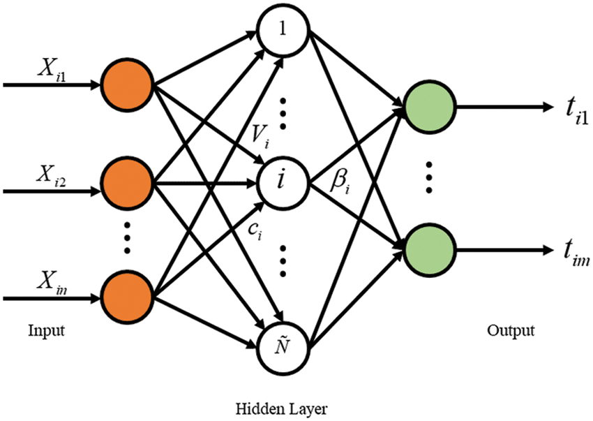
Figure 2: Structure of extreme learning machine

where n is the number of input data and m is the number of output data. The analysis is based on the ELM training process, with N training simples (Xi,ti), where Xi=[Xi1,Xi2,…,Xin]T is the input data and ti=[ti1,ti2,..,tim]T is the output data. The estimation of SLFNs is based on a mathematical model, given by

t^j=∑i=1N~βio(ci⋅Xj+Vi),j=1,2,…,N(9)

where ci=[ci1,ci2,..,cin]T is the input weight vector connecting of the i-th hidden and β=[βi1,βi2,…,βim]T is the output weight vector connecting of the i-th hidden neuron nodes, Vi is the bias of the i-th hidden neuron nodes, and o(∗) is the SLFNs’ activation function. In addition, unlike other machine learning algorithms, the ELM may create the input weight ci and bias Vi at random.

To increase regression performance, one of ELM’s abilities is to verify zero error, which may approximate all N simples as ∑i=1N‖t^j−tj‖=0, i.e. The N equations above can be expressed in a more compact form as

where β=[β1⋮βN~]N~×mT and T =[T 1⋮T N]N×mT(10)

=[o(c1⋅X1+V1)⋯o(cN~⋅X1+VN~)⋮⋯⋮o(c1⋅XN+V1)⋯o(cN~⋅XN+VN~)]N×N~(11)

where H is the neural network’s hidden layer output matrix and T is the training data target matrix.

β^ is the smallest norm least-square solution of the linear system provided by in the ELM solution.

β^=H P T (12)

where (∗)P is the Moore-Penrose pseudoinverse of H .

2.2.3.2 Regularized Extreme Learning Machine (RELM)

The ELM has performed well in a variety of applications; nonetheless, we believe that the method of N~ should be used to avoid overfitting and underfitting. Smaller norm parameters can provide higher generalization, according to the suggested RELM for SLFNs with sigmoid function detailed in the study. The equation may be used to many types of activation functions and hidden neuron nodes, such as kernels, to solve the issue in l2 norm of β.

As a consequence, RELM may be explained as a method by

minimize(β0,β)∈N~×1C2‖H β+β0−t‖22+(1−α)2‖β‖22+α‖β‖1,(13)

When just the l2 norm penalty (α=0) with β0=0 is considered, the RELM formula is given where C and β0 are regularization parameters.

β^=(H HH +IC)−1H Ht(14)

2.2.3.3 Outlier-Robust Extreme Learning Machine (ORELM)

The ORELM has recently been adjusted to increase performance in the l1 norm of techniques that create outliers. This may be accomplished using ELM, which is provided by

β^=argminβτ‖H β−t‖1,(15)

The solution to the following optimization is obtained by using the standard l2 norm.

β^=argminβτ‖H β−t‖1+12C‖β‖22(16)

Fig. 3 in the preparation process, information is essential for this work. This will divide the data preparation process. Two groups, the first group we call training data, are data preparation in massive MIMO systems with different values to require the algorithm to calculate and remember the values.

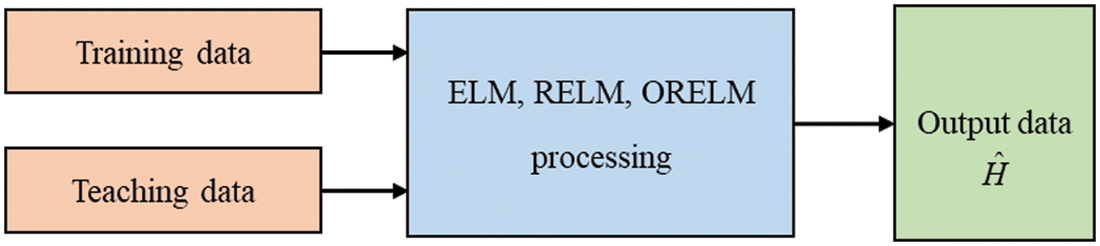
Figure 3: Preparation process for ELMx

The second group is called teaching data. In this group we want the algorithm to learn the desired value as a result. To distinguish the different values, we define it as the channel response of the massive MIMO communication system. After entering the data preparation process. In the workflow of the ELMx group’s algorithms, the steps are as follows

2.3 Mean Square Error

The performance of machine learning algorithms may be examined in a variety of ways. Consequently, we apply MSE in Performance Analysis to show a clear conclusion. This metric is widely used to evaluate performance and is based on the findings [9,10]. As a result, after computing all channel estimation algorithms, the error H^ is calculated, and the model forecasts the difference from the real H before finding the mean. We calculate the Gradient of Loss based on the difference and backpropagate the weight. Then, in the following training phase, we apply the Gradient Descent technique to decrease losses. The loss function in regression can given by

MSEN=∑i=1N‖H−H^‖2(17)

2.4 Estimated Channel Capacity

The theory of the data rate that can be accomplished over a certain bandwidth (BW) and at a specific signal to noise ratio is known as Shannon Capacity of a channel. It decreases the bit error rate (BER) that cannot be achieved in practice, but as link level design techniques improve, the data rate of noise channel approaches this theoretical bound [18]. The capacity in bps/Hz is expressed by

C=log2⁡det[IMR+PtPnMTHHH](18)

where IMR is identity matrix (MR × MR), H is channel response of size (MT × MR), (∗)H is transpose conjugate, and Pt/Pn is signal noise ratio (SNR).

To estimate the capacity of the channel, we looked at the channel responses obtained using LS, the popular MMSE method, and the other three based on the machine learning application is ELM, RELM, and ORELM techniques. The formula of estimated capacity is written by

Ces=log2⁡det[IMR+PtPnMTH^H^H](19)

where Ces is the estimated channel capacity, H^ is the estimated channel.

2.5 Outage Probability

The outage probability is another mostly performance index for communication techniques [19], in fading channel, can determines the probability of channel capacity under a certain rate which ensures data transmission without loss. The outage probability can be determined as

Pout(Ces<R)(20)

where R is the certain Rate of capacity.

As a result, the transmitter’s best option is to encrypt the data, given that the channel gain is sufficient to support the target rate R when this occurs, it is possible to achieve reliable communication, and otherwise an outage occurs. When the fading gain is h, think of the channel as allowing of information to pass through. As long as the amount of data exceeds the intended rate, reliable decoding is achievable. The outage probability of the Rayleigh channel given the transmission rate R is expressed by

Pout(R)=1−exp⁡(−2R−1SNR)(21)

where Pout denotes the outage probability of the system that the destination performs detection based only on the received signals from the relay node.

3  Result and Discussion

3.1 MSE and BER

In this section, we evaluate the mean square error (MSE) and bit error rate (BER), as well as the LS and MMSE channel estimates, to validate a group of ELMx algorithms. Massive MIMO systems use 128 transmitting and receiving antennas, each having its own QPSK modulation mapping and pilot number. Tab. 1 is explained the ELMx channel estimation technique. The result of MSE performance with all techniques as shown in Fig. 4. The LS technique was less effective than the 4 techniques presented. Since the method of obtaining the result is simple and uncomplicated, there is a large margin of error. MMSE technique, with the added complexity, makes it better than LS. Hence, we apply an approach to machine learning, a group we call ELMx, that outperforms LS and MMSE. This is because the ELMx base uses many datasets for training and testing to find results that are close to the target data.

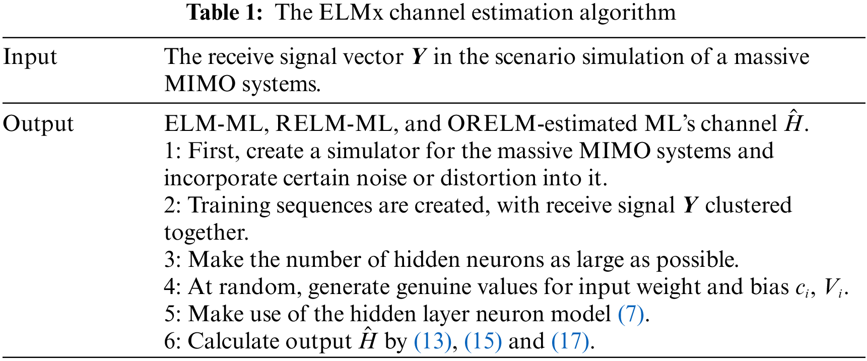
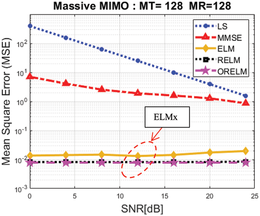
Figure 4: MSE performance in massive MIMO systems

Fig. 5. shows the BER performance results for all channel estimation. In a massive MIMO-based communication system, 128 transmitting antennas (MT) and 128 receiving antennas are considered (MR). The ELMx groups are better than the fundamental approaches of LS and MMSE channel estimation. The result reveal that BER performance of ORELM in ELMx group is the best performance.

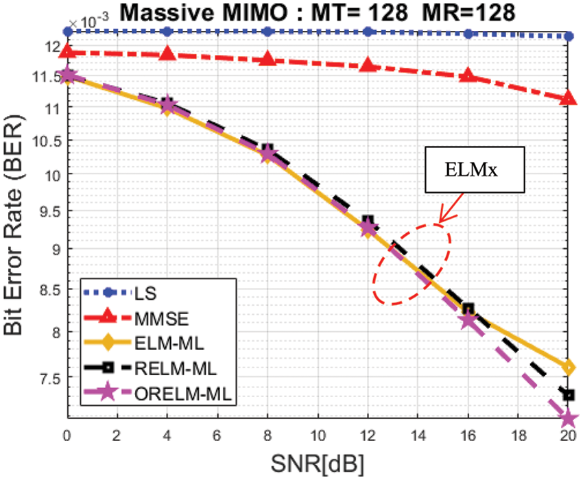
Figure 5: BER performance in Massive MIMO systems

3.2 Channel Capacity and Outage Probability

In this section, another measure of performance is channel capacity and outage probability in massive MIMO systems. Then we use Eq. (19) to process and comparing channel capacity, as shown in Figs. 6 and 7., use Eqs. (20) and (21) to process and finding outage probability.

The test result for channel capacity vs. SNR is shown that the traditional channel estimation LS and MMSE provides less channel capacity than ELM, RELM, and ORELM techniques. The group of ELMx is the best of channel capacity

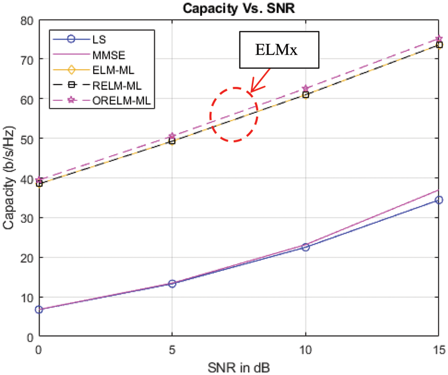
Figure 6: Channel capacity performance in massive MIMO systems

It is obvious that there is a very high probability that the capacity obtained for the massive MIMO channel is significantly higher than that obtained for an AWGN channel. The capacitance is insufficient compared to LS and MMSE, with a probability of 90% there is a capacity of 26 bps/Hz for LS and a capacity of 28 bps/Hz for MMSE. Therefore, we show the finding of high channel probability compared to LS and MMSE, with 90% of the probability. It has a capacity of 62 bps/Hz for ELM and RELM, with a capacity spacing of 34 bps/Hz for MMSE, so a good result and consistent with the method is ORELM as shown in Fig. 7.

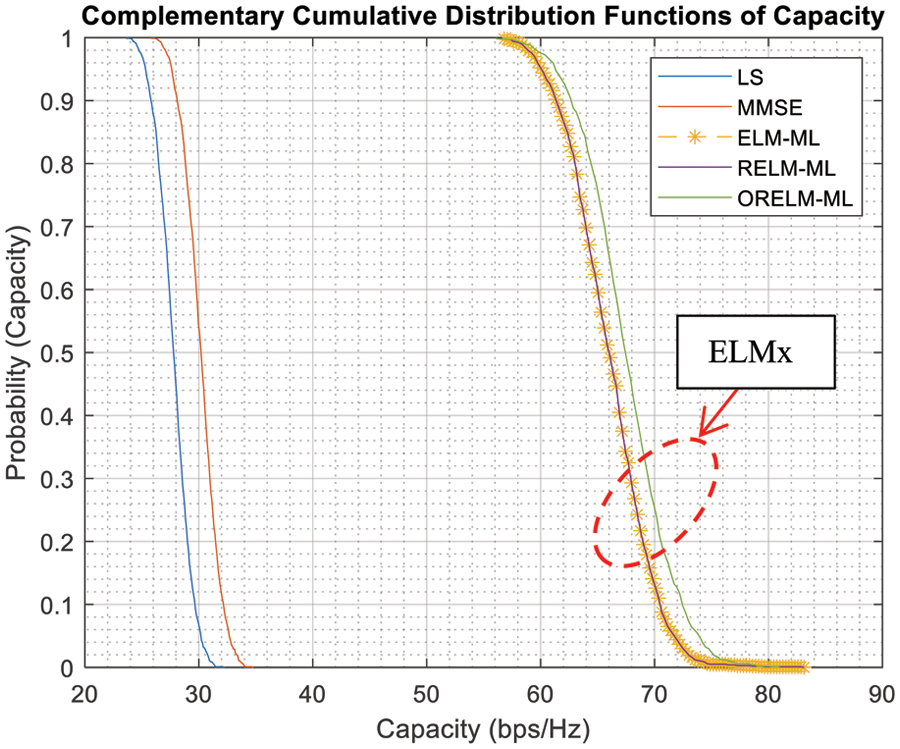
Figure 7: Outage probability performance of LS, MMSE and ELMx

3.3 Computational Complexity

In this section, many ways for defining complexity with the big O notation are covered in this section [20,21]. In terms of simpler functions, the big O notation indicates a function’s limiting behavior when its arguments go towards a given value. It’s part of a wider group of notices. The big O notation considers the largest of parameters, although some parameters cannot be cut off in this paper. Because the complexity in this work is dependent on a lot of variables, it aims to examine the delicate nature of the data by using the number of floating-point operations (flops) to substitute big O notations. A flop is here defined as one addition, subtraction, multiplication, or division of two floating-point numbers. It can be analyzed and shown in Tabs. 2–6.

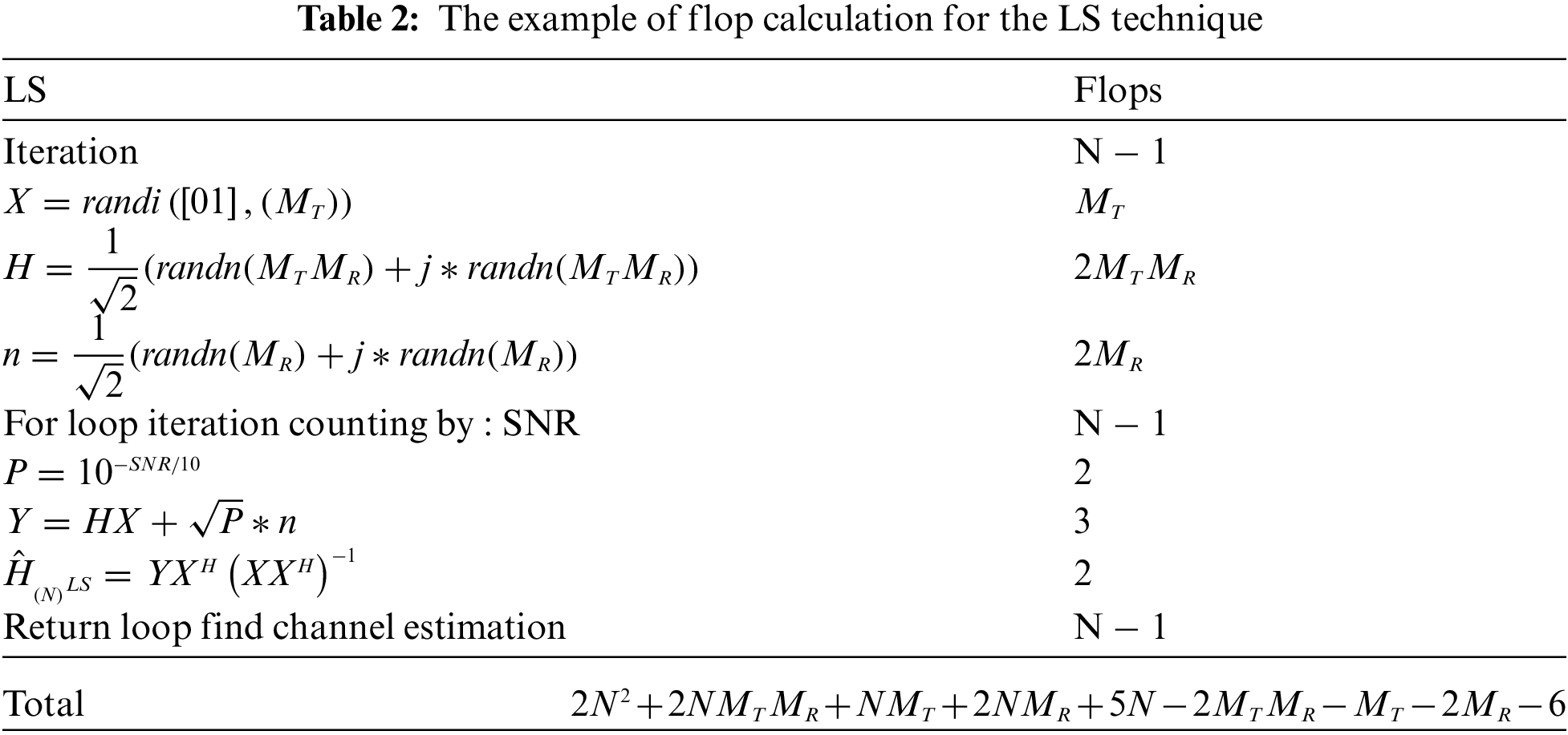
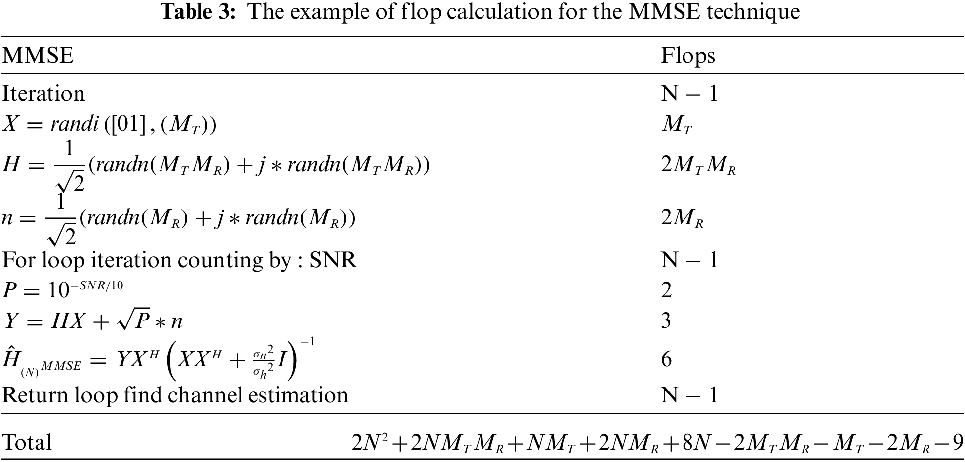
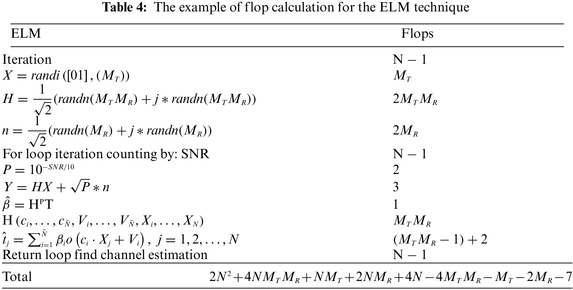
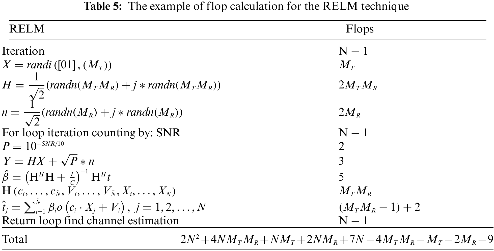
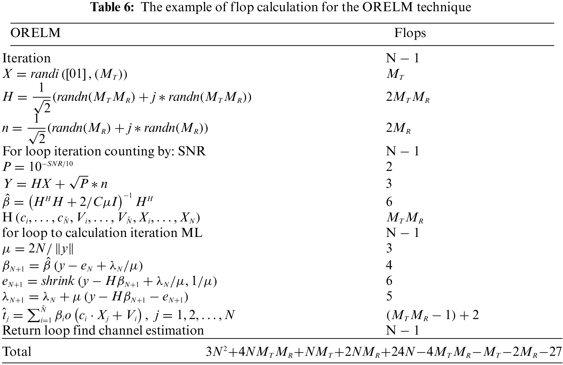
We took the total flops of each algorithm to calculate the number of bits of feedback and determined the number of massive MIMO antennas to determine the difference in flops and adjusted the number of loops. Another method for evaluating performance is computational time by using time as a measure of calculating various values to find the appropriateness of choosing to use as a result, we may be able to deploy and optimize or compare performance with other methods.

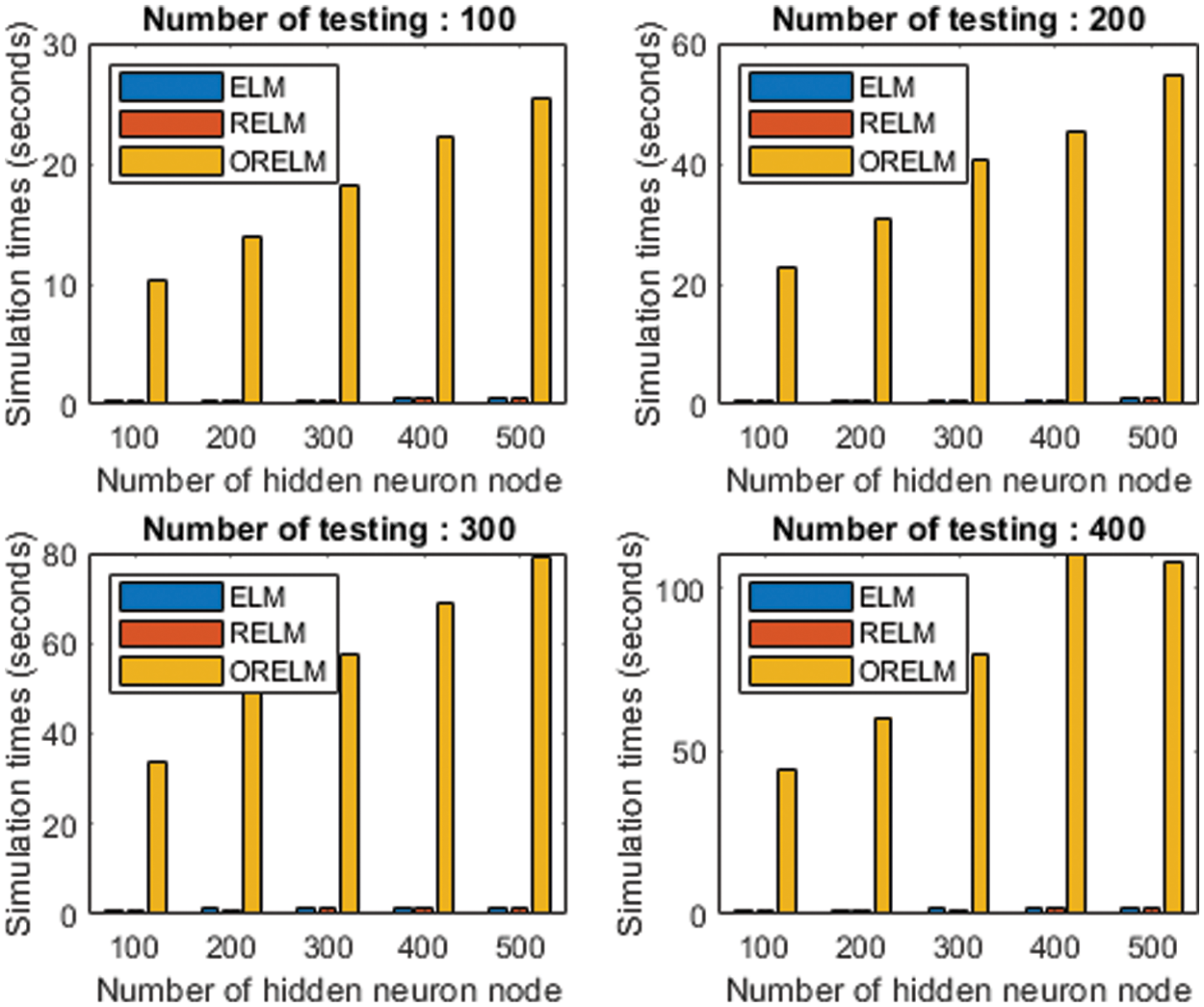
Figure 8: Computational time of ELMx

Fig. 8 shows that computational comparison between ELM and RELM, thus corresponding to the computational complexity for the number of nodes from 100 to 500 nodes, the computation time is clearly increased. The result of ORELM reveal that the computational time higher than ELM and RELM when the number of tests increases. Therefore, it make more clear in Fig. 9, we show the comparison between ELM and RELM in terms of computational time.

In terms of computational time, considering performance during the ELM and RELM algorithms, the RELM has a lower computational time than the ELM for all number of testing so, RELM is the best choice for future massive MIMO deployments.

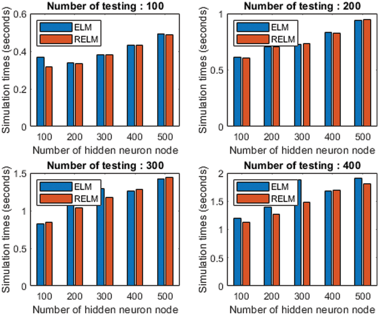
Figure 9: Computational time of ELM and RELM

4  Conclusion

In massive MIMO systems, adding more communication antennas and learning new techniques or procedures can help to improve the system or solve the problem. However, the problem may not be solved because there are multiple channels sent from the base station in the communication system. Therefore, this paper presented channel estimation techniques with machine learning based on massive MIMO systems. The authors apply various techniques to compare with LS, MMSE and ELMx groups. Three algorithms as ELM, RELM and ORELM are studied to test the efficiency of channel estimation. All results in terms of MSE, BER, Capacity, Outage Probability, analysis of computational time and analysis flop are confirmed that RELM was the best. This is because algorithm ORELM consumed longer data learning and testing time, while RELM algorithm spent lower data overfitting time. Therefore, in the future massive MIMO systems with ML, RELM is the best choice for channel estimation.

For future work, we plan to use the auxiliary information-aware ELM where phase [22], empirical mode decomposition [23], peak value of meditation [24], and wavelet transform decomposition [25,26] may be used as addition information to improve the performance of conventional ELM methods.

Funding Statement: This work was supported by Suranaree University of Technology (SUT) and Thailand Science Research and Innovation (TSRI).

Conflicts of Interest: The authors declare that they have no conflicts of interest to report regarding the present study.

References

 1.  N. C. Luong, P. Wang, D. Niyato, Y. Liang, Z. Han et al., “Applications of economic and pricing models for resource management in 5G wireless networks: a survey,” IEEE Communications Surveys & Tutorials, vol. 21, no. 4, pp. 3298–3339, 2019. [Google Scholar]

 2.  C. -L. I. C. Rowell, S. Han, Z. Xu, G. Li and Z. Pan, “Toward green and soft: A 5G perspective,” IEEE Communications Magazine, vol. 52, no. 2, pp. 66–73, 2014. [Google Scholar]

 3.  E. J. Oughton, K. Katsaros, F. Entezami, D. Kaleshi and J. Crowcroft, “An open-source techno-economic assessment framework for 5G deployment,” IEEE Access, vol. 7, pp. 155930–155940, 2019. [Google Scholar]

 4.  A. Zaib and S. Khattak, “Structure-based low complexity MMSE channel estimator for OFDM wireless systems,” Wireless Pers, vol. 97, no. 4, pp. 5657–5674, 2017. [Google Scholar]

 5.  A. F. Molisch, V. V. Ratnam, S. Han, Z. Li, L. Li et al., “Hybrid beamforming for massive MIMO: a survey,” IEEE Communications Magazine, vol. 55, no. 9, pp. 134–141, 2017. [Google Scholar]

 6.  J. Zhang, X. Yu and K. B. Letaief, “Hybrid beamforming for 5G and beyond millimeter-wave systems: a holistic view,” IEEE Open Journal of the Communications Society, vol. 1, pp. 77–91, 2020. [Google Scholar]

 7.  Q. Zhang, L. T. Yang, Z. Chen and P. Li, “A survey on deep learning for big data,” Information Fusion, vol. 42, no. 9, pp. 146–157, 2018. [Google Scholar]

 8.  Y. LeCun, Y. Bengio and G. Hinton, “Deep learning,” Nature, vol. 521, no. 7553, pp. 436–444, 2015. [Google Scholar]

 9.  H. Huang, J. Yang, H. Huang, Y. Song and G. Gui, “Deep learning for super-resolution channel estimation and DOA estimation based massive MIMO system,” IEEE Transactions on Vehicular Technology, vol. 67, no. 9, pp. 8549–8560, 2018. [Google Scholar]

10. C. Luo, J. Ji, Q. Wang, X. Chen and P. Li, “Channel state information prediction for 5G wireless communications: a deep learning approach,” IEEE Transactions on Network Science and Engineering, vol. 7, no. 1, pp. 227–236, 2020. [Google Scholar]

11. Z. Lian, L. Duan, Y. Qiao, J. Chen, J. Miao et al., “The improved ELM algorithms optimized by bionic WOA for EEG classification of brain computer interface,” IEEE Access, vol. 9, pp. 67405–67416, 2021. [Google Scholar]

12. W. Deng, Q. Zheng and L. Chen, “Regularized extreme learning machine,” in 2009 IEEE Symp. on Computational Intelligence and Data Mining, Nashville, TN, pp. 389–395, 2009. [Google Scholar]

13. G. Huang, H. Zhou, X. Ding and R. Zhang, “Extreme learning machine for regression and multiclass classification,” IEEE Transactions on Systems, Man, and Cybernetics, Part B (Cybernetics), vol. 42, no. 2, pp. 513–529, 2012. [Google Scholar]

14. K. Zhang and M. Luo, “Outlier-robust extreme learning machine for regression problems,” Neurocomputing, vol. 151, pp. 1519–1527, 2015. [Google Scholar]

15. G. R. Gaspar, M. Paulo and D. Rui, “Channel estimation in massive MIMO systems,” in FCT: DEE-Dissertações de Mestrado, pp. 28–30, 2016. [Google Scholar]

16. N. Promsuvana and P. Uthansakul, “Feasibility of adaptive 4×4 MIMO system using channel reciprocity in FDD mode,” in 14th Asia-Pacific Conf. on Communications, APCC, Akihabara, Japan, pp. 1–6, 2008. [Google Scholar]

17. P. Uthansakul and M. E. Bialkowski, “Multipath signal effect on the capacity of MIMO MIMO-OFDM and spread MIMO-OFDM,” in 15th Int. Conf. on Microwaves, Radar and Wireless Communications, MIKON, Warsaw, Poland, pp. 989–992, 2004. [Google Scholar]

18. A. Innok, P. Uthansakul and M. Uthansakul, “Angular beamforming technique for MIMO beamforming system,” in 9th Int. Conf. on Electrical Engineering/Electronics, Computer, Telecommunications and Information Technology, Phetchaburi, Thailand, pp. 245–248, 2012. [Google Scholar]

19. G. J. Foschini and M. J, Gans, “On limits of wireless communications in a fading environment when using multiple antennas,” Wireless Personal Communications, vol. 6, no. 3, pp. 311–335, 1998. [Google Scholar]

20. A. Innok, “Angular beamforming technique for mimo systems,” Diss. School of Telecommunication Engineering Institute of Engineering Suranaree University of Technology, 2013. [Google Scholar]

21. G. H. Golub and C. F. van Loan, Matrix computations. Oxford: North Oxford Academic, 1983. [Google Scholar]

22. K. Phapatanaburi, P. Buayai, W. Naktong and J. Srinonchat, “Exploiting magnitude and phase aware deep neural network for replay attack detection,” ECTI-EEC, vol. 18, no. 2, pp. 89–97, 2020. [Google Scholar]

23. K. Phapatanaburi, K. Kokkhunthod, L. Wang, T. Jumphoo and Uthansakul, “Brainwave classification for character-writing application using emd-based gmm and kelm approaches,” Computers Materials & Continua, vol. 66, no. 3, pp. 3029–3044, 2021. [Google Scholar]

24. T. Jumphoo, M. Uthansakul, P. Duangmanee, N. Khan and P. Uthansakul, “Soft robotic glove controlling using brainwave detection for continuous rehabilitation at home,” Computers, Materials & Continua, vol. 66, no. 1, pp. 961–976, 2021. [Google Scholar]

25. T. Jumphoo, M. Uthansakul and P. Uthansakul, “Brainwave classification without the help of limb movement and any stimulus for character-writing application,” Cognitive Systems Research, vol. 58, no. 1, pp. 375–386, 2019. [Google Scholar]

26. K. Kokkhunthod, T. Jumphoo and P. Uthansakul, “Improving brainwave classification for character-writing application using single effective EEG channel in SUT,” in Int. Virtual Conf. on Science and Technology. Nakhon Ratchasima, Thailand, 142–148, 2020. [Google Scholar]

This work is licensed under a Creative Commons Attribution 4.0 International License, which permits unrestricted use, distribution, and reproduction in any medium, provided the original work is properly cited.