DOI:10.32604/cmc.2022.027142
| Computers, Materials & Continua DOI:10.32604/cmc.2022.027142 | |
| Article |
Diabetes Prediction Using Derived Features and Ensembling of Boosting Classifiers
1School of Computing, SRM Institute of Science and Technology, Kattankulathur, Chennai, India
2School of Computing, Bharat Institute of Higher Education and Research, Chennai, India
3School of Computing, University of Eastern Finland, Kuopio, Finland
*Corresponding Author: R. Rajkamal. Email: rajkamar@srmist.edu.in
Received: 11 January 2022; Accepted: 04 March 2022
Abstract: Diabetes is increasing commonly in people’s daily life and represents an extraordinary threat to human well-being. Machine Learning (ML) in the healthcare industry has recently made headlines. Several ML models are developed around different datasets for diabetic prediction. It is essential for ML models to predict diabetes accurately. Highly informative features of the dataset are vital to determine the capability factors of the model in the prediction of diabetes. Feature engineering (FE) is the way of taking forward in yielding highly informative features. Pima Indian Diabetes Dataset (PIDD) is used in this work, and the impact of informative features in ML models is experimented with and analyzed for the prediction of diabetes. Missing values (MV) and the effect of the imputation process in the data distribution of each feature are analyzed. Permutation importance and partial dependence are carried out extensively and the results revealed that Glucose (GLUC), Body Mass Index (BMI), and Insulin (INS) are highly informative features. Derived features are obtained for BMI and INS to add more information with its raw form. The ensemble classifier with an ensemble of AdaBoost (AB) and XGBoost (XB) is considered for the impact analysis of the proposed FE approach. The ensemble model performs well for the inclusion of derived features provided the high Diagnostics Odds Ratio (DOR) of 117.694. This shows a high margin of 8.2% when compared with the ensemble model with no derived features (DOR = 96.306) included in the experiment. The inclusion of derived features with the FE approach of the current state-of-the-art made the ensemble model performs well with Sensitivity (0.793), Specificity (0.945), DOR (79.517), and False Omission Rate (0.090) which further improves the state-of-the-art results.
Keywords: Diabetes prediction; feature engineering; highly informative features; ML models; ensembling models
A person who lives longer with undiagnosed diabetes leads to damage of nerves, kidneys, blood vessels, eyes, and heart [1]. Therefore, It is essential for living well with diabetes is early detection which is the key to managing diabetes potentially and early preventing or delaying the serious health complications that can decrease quality of life. It is highlighted by researchers that data of the healthcare sector is growing faster than the data in financial services, manufacturing, and media industries. A compound annual growth rate (CAGR) of 36% will be experienced through 2025 is reported in [2].
Increased amounts of healthcare data and the availability of historical healthcare data naturally ease the process of early detection of diseases with the help of ML techniques. Numerous data sources are available for diabetes-related data. Government healthcare organizations of several countries made the diabetes-related data available for open access. In addition to that, UCI ML repository [3], Kaggle [4], Data world [5], Amazon’s data sets [6], Google’s data sets [7] are the sources where diabetes-related data are available. Different data sets (historic data) have different attributes (features) which are recorded manually or by electronic equipment. In recent years, various ML models have been developed around the available datasets for diabetes prediction. Decision Trees [8] Random Forest (RF) [9], Logistic Regression (LR) [10], Naive Bayes (NB) [11], Support Vector Machine (SVM) [12], Artificial Neural Network (ANN) & Deep Learning [13] and AB [14] are few notable models using various dimensionality reduction and cross-validation techniques were proposed. Authors of [8–14] used various data sets for preparing and analyzing the performance of ML models. PIDD is a widely used dataset by several researchers in model developments of early prediction of diabetes. It has 8 features. However, real-time diabetes databases have more features on diabetes. Few notable state-of-the-art works of FE applied on the diabetes dataset are reviewed in Tab. 1.
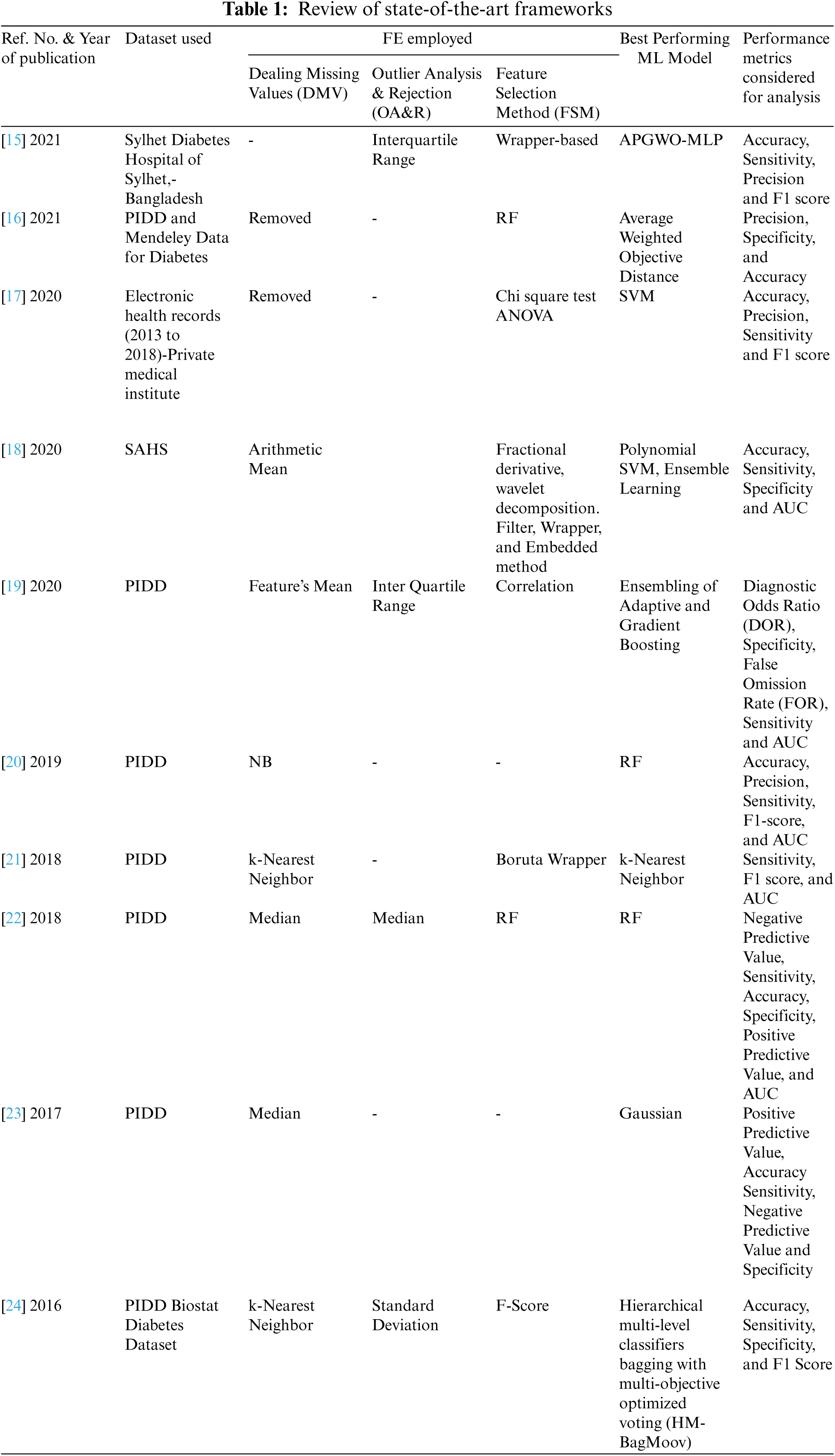
From Tab. 1, it is clear that FE techniques take a seat between data and ML models and it is given more importance in refining the performance of ML models in the detection of diabetes. Several researchers thrived to advance the performance of the ML models with different combinations of techniques of FE. From the listed state-of-the-art frameworks listed in Tab. 1, it is clear that the taxonomy of FE includes dealing with MV, pervading domain knowledge, introducing/removing dummy attributes, dealing with categorical attributes, creating interactive and new attributes from the existing raw attributes, and removal of unused/unwanted attributes. State-of-the-art results, particularly demonstrated [15] that an ensemble of ML models with suitable FE techniques are having the ability to outperform the standalone ML models. Different performance metrics are used to assess the ML models and also the entire framework (ML pipeline) for the accurate detection of diabetes. The most widely used metrics are accuracy, F1 score, precision, sensitivity (or recall), False Positive Rate (FPR), specificity, ROC-AUC, and True Positive Rate (TPR). In addition to these parameters, FOR and DOR is pivotal metric needed to be used to evaluate the classifier in disease diagnosis-related problems. However, only a few parameters are used to evaluate the models’ performance in any of the tabulated (Tab. 1) state-of-the-art frameworks.
From the above discussion, it is clear that though several state-of-the-art frameworks were available on the detection of diabetes at the primary stage, improvements are still required in terms of performance to bring the robustness of the ML models. A novel FE framework with an ensemble model is proposed in this work, to push on the models’ performance in diabetes diagnosis. The novelty and the contributions of this proposed framework are as follows.
• Imputation of MV is carried out based on mean or median or regression to preserve the Gaussian distribution of individual features. This process of imputation varies with the features and its impact on the performance measures of the ML model are analyzed.
• Permutation importance and partial dependence are used to calculate the relative importance scores that are independent of the models. Experiments were carried out extensively to identify the highly informative features. The highly informative features are examined with DT and RF models to analyze its dominance on the outcome of the model.
• Experiments are conducted on ensemble classifiers (AB and XB) with and without derived features (in addition to existing features of PIDD). Results are compared with the existing state-of-the-art works.
The organization of this paper is that the detailed study of the dataset, proposed framework, analysis of the impact of the imputation of MV, and dealing of outliers are discussed in Section 2.1. The impact analysis of derived features, permutation importance, and partial dependence analysis is discussed in Section 2.2. The details of the experimental results obtained to analyze the performance of the different ML classifiers and the comparative study of the proposed framework with state-of-the-art frameworks are discussed in Section 3 followed by the conclusion & future work in Section 4.
2.1 Dataset, Imputation of MV and Dealing Outliers
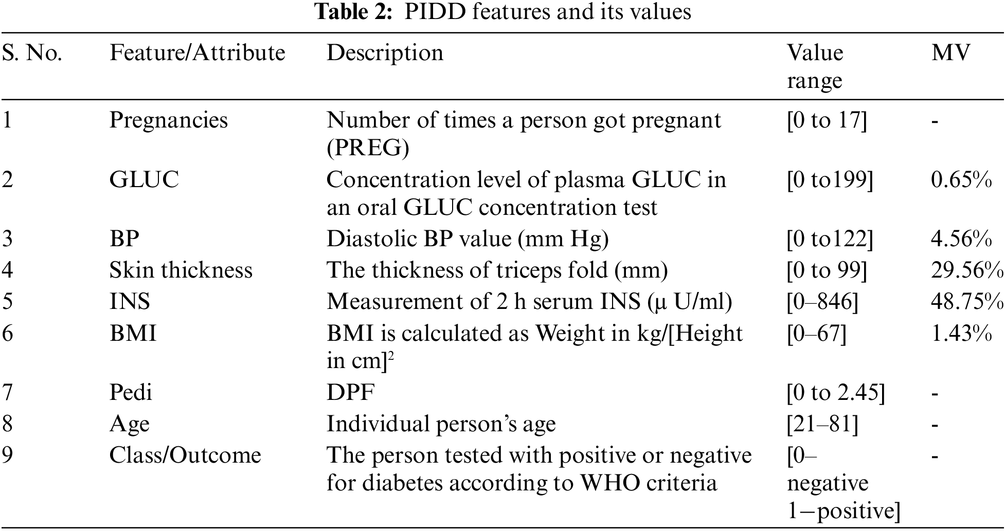
The central data repositories of the National Institute of Diabetes and Digestive and Kidney Diseases (NIDDK) [25] enable the researchers to carry out several studies to test many new hypotheses with the available data collection. PIDD is originally derived from the central data repository of NIDDK. After applying several constraints on the database of people living near Phoenix, Arizona of the Pima Indian population, PIDD is curated to have females of 21 years old at least, from Pima Indian heritage. Healthcare variables namely Pregnancy, GLUC, Skin Thickness, Blood Pressure (BP), INS, BMI, and Diabetes Pedigree function (DPF) are present in the dataset. In addition to the healthcare variables, there is a class variable (outcome) describing whether the patient tested for diabetes is positive or negative based on the World Health Organization (WHO) criteria. The range of values of class variables with the description of the variables of PIDD is given in Tab. 2. 768 instances were considered in the PIDD. The data set contains 34.9% (i.e., 268-number of diabetic patients) instances of diabetic people’s data and 65.1% (i.e., 500-number of non-diabetic patients) instances of non-diabetic (healthy) people’s data.
The proposed FE pipeline is summarized and illustrated in Fig. 1.

Figure 1: Proposed FE pipeline
Tab. 2 illustrates the percentage of MV for all features in the dataset. INS and skin thickness features are having the highest percentage (48.75% and 29.56% respectively) of MV. MV for each feature required to be dealt with different strategies as it has its impact on the outcome (healthy or diabetic). Treatment and Diagnosis for the patient are truly carried out based on the data. Missing data may end up drawing an inaccurate inference about the data and it may affect the process of the curative and findings that the patient should get [26]. In general, the minimum value for most predictors is zero, and it doesn’t make any sense in the healthcare domain. Therefore, zero is also considered as an indicator of absent values. In this FE pipeline, MV (zeros) are considered as Not a Number (NaN) for further processing of data. To address this problem of MV imputation, several techniques have been impelled in statistics and ML. Literature [27–30] discloses that the nature of variables, number of variables, and number of cases in the problem domain result in the effectiveness of the proposed methods and thus there is no straightforward strategy that guarantees one method over the others. Therefore, it is essential to have statistical insight into features before performing the imputation process.
From Tab. 3 minimum and maximum parameters indicate the low and high values in the data set of the corresponding medical predictor features respectively. The range is the measure of dispersion, which gives the difference between the maximum and minimum value of the variable. Further, Median Q1, Q3, and IQR (Q3–Q1) values of each feature are providing meaningful insights into data. Box plot represents the statistical values (Maximum, Minimum, First Quartile, Median (Second Quartile), and Third Quartile values) of each feature. Fig. 2 shows the box plot representation for each of the features available in the PID. For each feature, the name of the feature is mentioned in the x-axis and its statistical five summary values on the y-axis. Fig. 2, highlights the outliers (exists in skin thickness, BP, and BMI) existing in each feature to be dealt with using feature engineering. Based on IQR the identified outliers are removed. This process yields 636 instances of the dataset (132 instances are removed from 768 instances).
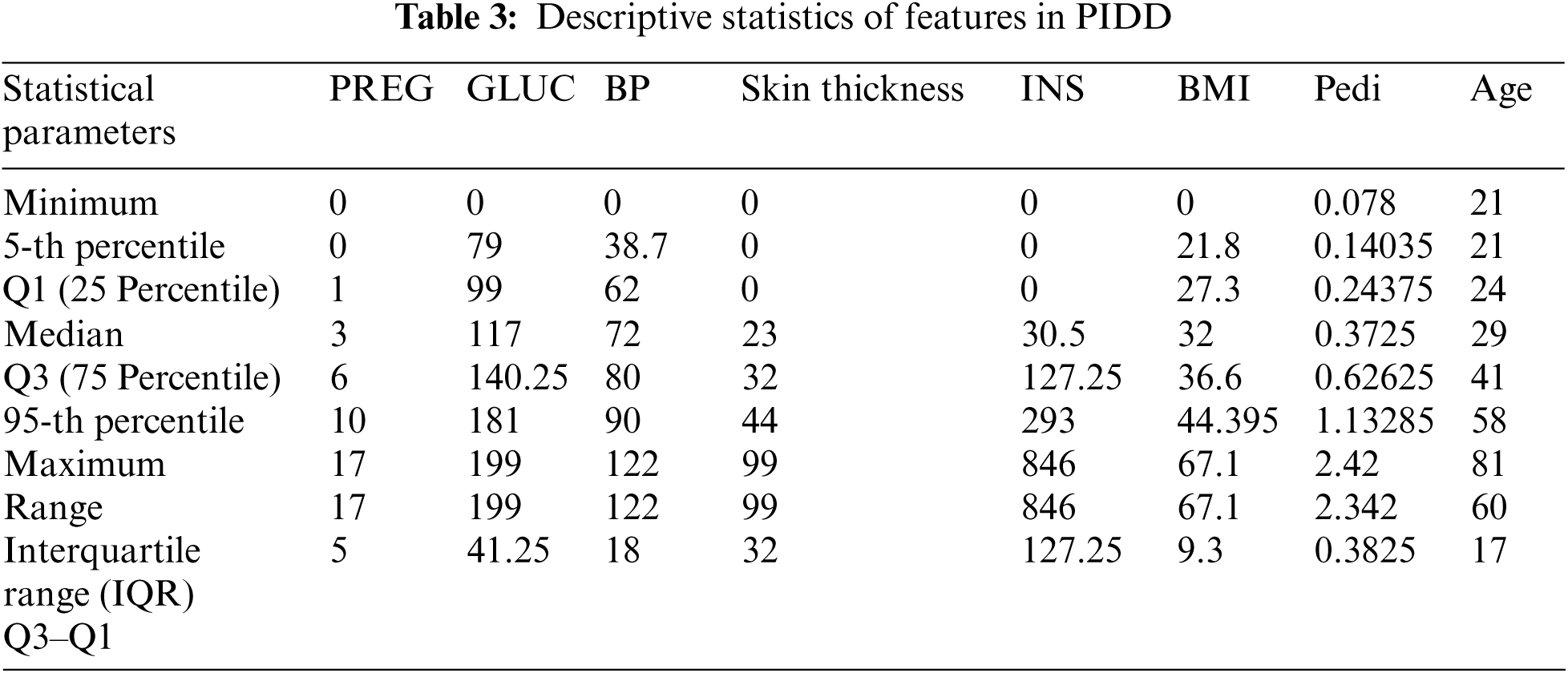

Figure 2: Outlier analysis of PIDD features
In general, when outliers are present in the features, imputation of missing value is carried out with the median value of the respective feature. Therefore, Skin thickness, BP, and BMI are imputed with the respective features’ median value and other features (GLUC and INS) are imputed with mean values. This imputation technique works better when the data size is small. However, for the larger dataset, imputing MV with central tendencies like mean, the median will add variance and bias in the dataset. This leads to overfitting or underfitting during the training phase of the ML model. In this scenario, the ML model itself is used here to impute the MV. The features of PIDD with MV are considered as target variables and the other features with no MV are considered as predictor variables. The choice of ML model for predicting the MV is decided based on the relationship exhibited between features.
The following relationship evinces among the features of PIDD from Fig. 3,
• GLUC manifests a positive weak linear association with all other features. This indicates an increase in the GLUC level of patients will lead to an increase of all other features’ value.
• BP manifests a positive weak linear association with all other features. This indicates an increase in the BP level of patients will lead to an increase of all other features’ value.
• Skin thickness manifests a positive weak linear association with all other features except Age. Skin thickness with Age manifests a weak negative correlation. This indicates that an increase in skin thickness leads to an increase of all other features value and a decrease in Age.
• INS manifests a positive weak linear association with all other features except Age. INS with Age manifests a weak negative correlation. This indicates that an increase in INS leads to an increase of all other features value and a decrease in Age.
• BMI and DPF also manifest a positive weak linear association with all other features.

Figure 3: Correlation (relation) exist among the features
From the above discussion, it is evident that all features (except Age) exhibit linear relation with other features in the dataset. This gives an intuition to use multi-variable linear regression to impute the MV. In PIDD, GLUC, INS, BP, skin thickness, and BMI are the features having MV. Using a regression model, to impute a feature using other features (having MV) is not possible. Therefore, all the features having MV are imputed with random values (by ignoring all other features) then the regression model is applied for imputation iteratively. This procedure is repeated for all the features having MV by considering the imputed feature as a predictor to evaluate the other features. Initially, the random values are imputed (without considering other features) which will not help to improve the ML model performance in the training phase. To overcome this, instead of imputing random values initially, Gaussian noise (with mean = 0) is added. This imputes negative values and zeros due to the nature of data distribution. In PIDD, features like GLUC and INS having negative values would be meaningless. For such values alone, random imputation is performed. Though this process reduces the spread of data distribution, it is essential to impute meaningful values in real-time for the features like INS and GLUC.
Fig. 4 shows the data distribution (before and after imputation with different mean, median, and regression) of PIDD features. Features with MV (INS, GLUC, skin thickness, BP, and BMI) are imputed with their respective mean/median and random regression values to demonstrate the impact of imputation to explore whether the features exhibit Gaussian distribution. Median value imputation is only to be considered for the features having outliers. It is observed from Fig. 4 (ref col 2 and 3) the variance of feature reduces after imputing median values of respective features. Imputed median values are mere estimates and it does not indicate any relation with any other features of the dataset. Further, from Fig. 4, it is clear that INS, GLUC, and skin thickness features are not yielding Gaussian distribution for the features after median imputation. So the regression imputation method is considered for INS, GLUC, and skin thickness and examined for Gaussian distribution, even though for INS, Gaussian distribution is not perfectly achieved through Regression Imputation, as the feature is missing the majority of its data. From the above analysis, it is concluded that BP and BMI are imputed with median values, INS, GLUC, and skin thickness are imputed with regression values.
Fig. 5 shows the variance measured for PIDD features. From Figs. 4 and 5, it is clear that the chosen independent features are having a high correlation with dependent features in regression imputation. Also, this results in considering the linear relationship between the features. This may not hold in reality. Particularly, the relationship between INS and GLUC is different for healthy and diabetic patients. Since the relationship between each feature is known from correlation, this problem is addressed by derived features from one or more available high-quality informative features.
2.2 Impact Analysis of Derived Features
The derived feature is more useful and it can add more information than using the feature in its raw form. The process of deriving features from the existing features of the dataset is performed to add important features to the dataset to discover effective information from different perspectives. Feature importance is the method to understand the relative significance of the features in the model’s performance. Feature importance [31] is used to examine the change in out-of-sample predictive accuracy when each one of the features is changed. Feature importance score is obtained using decision tree (Fig. 6a) and RF (Fig. 6b) models. From Fig. 6, it is clear that the GLUC feature is having high feature importance scores when compared with the other features of PIDD, the second important feature is the BMI feature and the third is the INS.
Since the size of the selected important input feature set is small, the partial dependence analysis is carried out to justify the selected important features’ interaction with the target (outcome). The partial dependence of the features is the result of the computation of integral of various data. The target at any point is given in terms of the partial dependence of the features. This shows the effect of features in prediction. In this work, two non-linear ML models, the DT classifier and RF classifier are considered for the impact evaluation analysis of selected features. The selected features are GLUC, BMI, and INS.
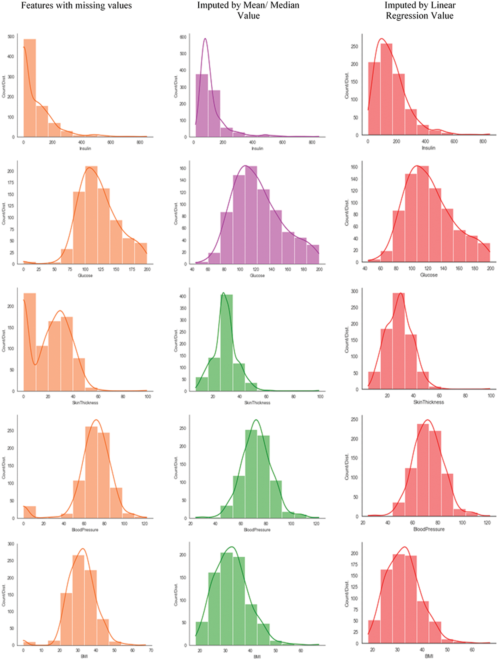
Figure 4: Data distribution of PIDD features having MV (before and after imputation using mean/median and regression techniques)

Figure 5: Data distribution (before and after imputation) of PIDD features

Figure 6: Feature importance score of PIDD feature used with (a) DT (b) RF
Fig. 7a shows the level of confidence of the decision tree classifier in predicting diabetes. It is observed that increasing the level of GLUC substantially increases the chances of having Diabetes but GLUC levels beyond 160 appear to have little impact on predictions. From Fig. 7b, it is evident that when the BMI value is between 28 and 42 it has a very little impact on predictions. But when BMI value is beyond 42, it substantially increases the chance of diabetes. From Fig. 7c, it is evident that the INS less than 140 on average indicates no diabetes, and its value after 200 has no impact on predictions.

Figure 7: Partial dependence of GLUC, BMI, and INS in DT classifier’s outcome (healthy/diabetic)
In Fig. 8, the predicted outcome of the model is given against the feature and the shaded area indicates the level of confidence of the RF classifier in predicting diabetes. From Fig. 8a, it is observed that the increase in GLUC level substantially increases the chances of having diabetes, also it is observed that the GLUC level > 160 appears to have less impact on the RF classifier model predictions.
It is evident from Fig. 8b that for BMI values between 28 and 42, very little impact in improving the confidence level of predictions of the RF classifier predictions. However, for BMI > 42, it substantially increases the confidence level of prediction of diabetes. From Fig. 8c, it is evident that the INS less than 140 on average indicates no diabetes, and its value after 200 has no impact on predictions.


Figure 8: Partial dependence of GLUC, BMI, and INS in RF classifier’s outcome (healthy/diabetic)
From both Figs. 7 and 8, it is clear that the selected features (GLUC, BMI, and INS) show a dominant impact in the prediction of healthy/diabetic irrespective of the choice of ML model. GLUC feature is categorized as a high-quality informative feature and therefore, BMI and INS are considered for deriving the features to add more information.
2.2.1 Case 1: Derived Feature 1-BMI
The healthy range for BMI [32] is between 18.5 and 24.9. BMI value under 18.5 is considered underweight and possibly malnourished; 25.0 to 29.9 are considered as overweight and over 30 are considered as obese. By keeping the WHO’s guideline, the BMI feature in PIDD is analyzed and the following are observed in the PIDD and shown in Tab. 4.

The BMI feature is synthesized into 4 categories namely underweight, healthy, overweight, and obese, and the number of patients falling under each category is shown in Tab. 4. A new set of derived features are formed based on the synthesized 4 categories and named BM_Desc_under, BM_Desc_healthy, BM_Desc_over, and BM_Desc_obese. BM_Desc_under has only 4 instances. Therefore, it is not considered for further analysis. In [32], the authors reported the causal result of a rise in the BMI on the likelihood of being diabetic and also described the relation between BMI and diabetes.
2.2.2 Case 2: Derived Feature 2-INS
Generally, the INS level is assessed after fastening for a considerable duration. INS feature in PIDD is the measurement taken against 2-h serum INS (mU/ml). INS value between 16 and 166 is considered as normal INS level for 2-h after GLUC. Based on this value, INS features are analyzed and the following are observed in the dataset. The INS feature is synthesized into 2 categories namely normal and abnormal. The number of patients falling under each category is shown in Tab. 5. A new feature is formed based on these 2 categories and named Insulin _Desc_normal and Insulin _Desc_abnormal. The level of INS in the bloodstream will vary following the level of GLUC.


Figure 9: (a) & (b) Effect of derived features of INS (in relation with other features) on the outcome (healthy = 0/diabetic = 1)
The derived features, Insulin _Desc_normal and Insulin _Desc_abnormal are directly related to outcome (target). Since INS is highly rated in feature importance, the relationship of the derived features with other features (BP and GLUC, BP and DPF) concerning outcome is analyzed. Figs. 9a & 9b clearly depicts this scenario. From Fig. 9a, for the BP (value between 70 and 120), It is seen that the Insulin _Desc_normal (values between 50 and 170) and GLUC level (between 100 and 190) results in the outcome of 0 (healthy). Similarly Insulin_Desc_abnormal (values between 100 and 180) and GLUC level (between 100 and 190) results in the outcome of 1 (diabetic). Fig. 9b depicts the derived features. Insulin_Desc_normal and Insulin_Desc_abnormal impact in the outcome for the other features BP and DPF. For the BP (value between 70 and 120), it is seen that the Insulin_Desc_normal (values between 50 and 170) and DPF (< 1) results in the outcome of 0 (healthy). Similarly, Insulin_Desc_abnormal (values between 100 and 180) and DPF (>0.5) results in an outcome of 1 (diabetic). This clearly shows the direct impact of Insulin_Desc_normal and Insulin_Desc_abnormal on the outcome. From the above discussion, it is evident that the derived features are not only providing insights into the respective features but also have a direct relationship with the outcome. However, irrespective of feature or derived feature, it is vital to evaluate the features for their impact on the ML model in the early prediction of diabetes
Identifying the quality features and adding more information with the existing features using derived features are described in the previous section. In this section, to show the importance of the features including derived features, the permutation importance of features of PIDD is calculated using an RF classifier. With multiple shuffles, the permutation importance calculation is achieved and the amount of randomness is measured. The importance of features is listed in Tab. 6 in the order from top to bottom. The first decimal in each row indicates how much model performance is decreased with a random shuffling. The number after the ± measures indicates the variation in model performance in one-reshuffling to the next. In shuffling a respective feature, randomness is involved in exact performance change. Negative values are occasionally seen for permutation importance where the predictions on the shuffled feature happened to be more accurate than the real data. The randomness produced the predictions on the shuffled feature and the feature with importance close to 0 is to be more perfect.

In Tab. 6, the feature shown in green indicates that it has a positive impact on prediction and subsequently the change in green color indicates less impact than the dark green marked feature (GLUC). The feature (BM_DESC_obese) shown in white indicates that it doesn’t have any effect on our prediction. The permutation feature importance technique is biased for unrealistic instances of features in the case where features are more correlated with another feature.
The attributes mean/median/regression imputation for missing value imputation, IQR for outlier rejection, and permutation importance weight for feature selection are considered in the proposed FE. As a result of the process discussed in the previous sections, there are 7 actual features and 6 derived features from PIDD are obtained with positive weights of permutation (Tab. 6). Skin Thickness is the feature having a negative weight of −0.021 ± 0.0169. It is dropped from the dataset as it is not having much impact on diabetes prediction. The proposed FE is applied on the PIDD and 7 features (except Skin Thickness) and 5 derived features (except BM_Desc_under) with 636 instances are obtained. Further, the PIDD is divided into training and testing samples using 5 fold stratified K-fold cross-validation, where each fold is preserving the percentage of data samples from healthy and diabetic classes. The authors of [19], conducted experiments on different ensemble models for increasing the performance of the prediction of diabetes. From the experiments, the authors reported that the AB and XB model combination provides the supreme prediction of diabetes when compared with the other state-of-the-art methods. Therefore, the same ensemble model combination (i.e., AB + XB) is considered with the model regulating parameters as shown in Tab. 7.

The diabetes prediction results obtained for the combination of AB and XB are shown in Figs. 9a and 9b. Sensitivity, Specificity, DOR, FOR, and AUC are considered as key evaluation metrics for assessing the performance of the classification of ML models. AUC is the metric that is unbiased to the class distribution. Therefore, AUC is given more importance rather than accuracy. However, all the other metrics can also be obtained from the confusion matrix (Fig. 10b). The performance evaluation of the ensemble model is analyzed for 7 features + 1 derived feature (Insulin_Desc_Normal (or) Insulin_Desc_Abnormal), 7 features + 2 derived features (Insulin_Desc_Normal and Insulin_Desc_Abnormal), and 7 features + 4 derived features (Insulin_Desc_Normal, Insulin_Desc_Abnormal, BM_Desc_healthy, and BM_Desc_over) and the respective key performance metrics are obtained and tabulated in Tab. 8.
The combination of the ensemble model (AB + XB) with the proposed FE method, particularly with 4 derived features (ref Tab. 8, row 4) shows the dominance in 3 metrics out of five. The best values (each metric) are highlighted with an underline. From Fig. 10a, AUC-ROC Curve, It is observed that the False Positive Rate (FPR) of 0.043 is leading to the possibility of getting True Positive Rate (TPR) of 0.793 (indicated with a red star in the AUC-ROC curve) in model’s accuracy. Though the AUC for the combination of 2 derived features (ref Tab. 8, row 3) is equal, the DOR of 117.694 is high by the margin of 8.2%. DOR is the prevalence measure and it is considered as one of the best metrics in disease diagnosis (diabetes prediction). The inclusion of more highly weighed permutated derived features leads to an increase in the DOR which demonstrates the impact of derived features in model performance. Not only the DOR but the specificity and AUC also show good impact (increasing) for the inclusion of derived features (ref Tab. 8, columns Specificity and AUC).
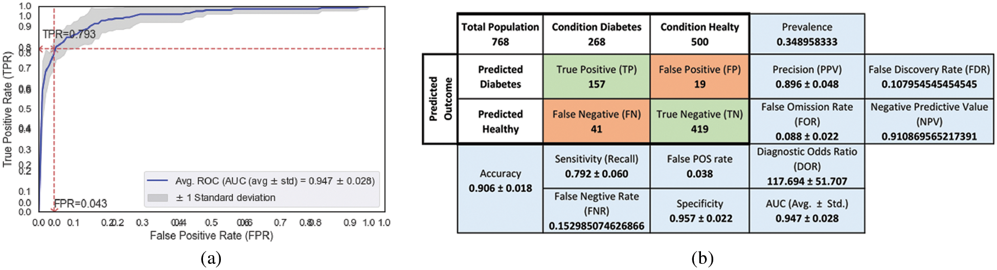
Figure 10: Performance metrics of ensemble (AB + XB) model with 7 features obtained from the proposed FE (for Tab. 8, row 4) (a) AUC-ROC (b) Confusion matrix

Further, to demonstrate the impact of derived features in the model’s performance; an experiment is carried out with the prevailing state-of-the-artwork reported in [19]. In [19], the attribute’s mean for missing value imputation, IQR for outlier rejection, and correlation for feature reduction are reported as FE. After this process, the authors arrived with 6 features with 636 instances arriving from PIDD. The values of the 3 performance metrics (Sensitivity, FOR, and AUC) (out of five metrics) are reported as better than the other combination of ensemble models. These values are reported in Tab. 9 (row 1). In this work, the derived features are included and their impact on model performance is analyzed with the ensembling model (AB + XB) performance for the FE reported in [19].
The performance evaluation of the ensemble model is analyzed for 6 features + 1 derived feature (Insulin_Desc_Abnormal (or) Insulin_Desc_Normal), 6 features + 2 derived features (Insulin_Desc_Normal Insulin_Desc_Abnormal) and 6 features + 4 derived features (Insulin_Desc_Normal Insulin_Desc_Abnormal, BM_Desc_healty, BM_Desc_over, and the respective key performance metrics are obtained and reported in Tab. 9.

From Fig. 11a, AUC-ROC Curve, It is observed that the FPR of 0.055 is leading to the likelihood of getting TPR of 0.793 (indicated with a red star in the AUC-ROC curve) in model’s accuracy. The combination of the ensemble model (AB + XB) with the FE method reported in [19], particularly the inclusion of 1 derived feature (ref Tab. 9, row 2) shows the dominance in 4 metrics out of five. Though the AUC is less when compared with the inclusion of no derived features (ref Tab. 9, row 1), the Sensitivity, Specificity, and DOR are high by the margin of 0.4%, 0.1%, and 13.9% respectively. The less FOR value (0.090 ± 0.017) (ref Tab. 9, row 2, column FOR) yielded by the high negative prediction values (predicted healthy), which leads to less Type-2 error in diabetes prediction.

Figure 11: Performance metrics of ensemble (AB + XB) model with 6 features obtained as reported in [19] + 1 derived feature (for Tab. 9, row 2) (a) AUC-ROC (b) Confusion matrix
From the above discussions, It is conclusive that the inclusion of high weighted permuted derived features is making an impact in providing the better performance of the ensembling model (AB + XB) as the model has the advantage of both sequential boosting (AB) and parallel boosting (XB). From the above discussion, it is clear that the inclusion of derived features is certainly increasing the performance of current state-of-the-artwork as well. Further, to validate the projected ML pipeline and classifiers performance on diabetes prediction are compared with a few other state-of-the-art works.
From Tab. 10, it is observed that all the state-of-the-art frameworks (used PIDD) are not considered all the 6 metrics (except [19]) though they treated the prediction of heart disease problem as a binary classification problem. In [23] and [20] the information on outlier analysis/rejection and FSM are not reported. From Tab. 10, it is clear that all the models’ accuracy looks improved in the prediction of diabetes. The FE pipeline proposed with the ensembling model is outperformed other works with improvement in terms of accuracy or AUC or both. The inclusion of the derived features in the feature selection stage of the ML pipeline ensures the addition of more information with the existing features leads to improved accuracy and AUC when compared with other state-of-the-art works. The high value of DOR shows the discriminative power of the ML model in the prediction of diabetes. The inclusion of derived features with the existing state-of-the-art FE approach [19] made the ensemble model performs well with Sensitivity (0.793), Specificity (0.945), DOR (79.517), and FOR (0.090) which improved the state-of-the-art results.

FE has its impact on healthcare domain data particularly in the diagnosis and prognosis of diseases. The importance of exploratory data analysis in terms of concluding on MV, imputing MV, the effect of imputation in diabetes prediction are discussed. It is shown that the imputation process is helping ML models in early prediction by changing the distribution of data. The effect of constructing new features from the existing features and their importance in the ML model is analyzed. The impact of GLUC, INS, and BMI features are studied with DT classifier and RF classifier models. Irrespective of the choice of the ML model, the selected quality features (GLUC, INS, and BMI) showed their dominant impact on the outcome (diabetes/healthy). The impact analysis of the derived features with the ensembling model (AB + XB) demonstrates that the inclusion of the derived features outperforms the model with no inclusion of derived features and also advances the state-of-the-art results. The proposed method shall be used in other diagnosis problems as well in the healthcare domain.
Funding Statement: The authors received no specific funding for this study.
Conflicts of Interest: The authors declare that they have no conflicts of interest to report regarding the present study.
1. J. Fisher-Hoch, S. P. Vatcheva, K. P. Rahbar and H. McCormick, “Undiagnosed diabetes and pre-diabetes in health disparities,” Plos One, vol. 10, no. 7, pp. e0133135, 2015. [Google Scholar]
2. F. Donovan, “Organizations see 878% health data growth rate since 2016,” https://hitinfrastructure.com/news/organizations-see-878-health-data-growth-rate-since-2016. 2019. [Google Scholar]
3. UCI machine learning repository, https://archive.ics.uci.edu/ml/index.php. [Google Scholar]
4. Kaggle, https://www.kaggle.com/datasets. [Google Scholar]
5. Data world, https://data.world/. [Google Scholar]
6. Amazon’s datasets, https://registry.opendata.aws/. [Google Scholar]
7. Google’s datasets, https://datasetsearch.research.google.com/. [Google Scholar]
8. I. Jenhani, N. B. Amor and Z. Elouedi, “Decision trees as possibilistic classifiers,” International Journal of Approximate Reasoning, vol. 48, no. 3, pp. 784–807, 2008. [Google Scholar]
9. L. Breiman, “Random forests,” Machine Learning, vol. 45, pp. 5–32, 2001. [Google Scholar]
10. B. P. Tabaei and W. H. Herman, “A multivariate logistic regression equation to screen for diabetes: Development and validation,” Diabetes Care, vol. 25, no. 11, pp. 1999–2003, 2002. [Google Scholar]
11. G. Webb, J. Boughton and Z. Wang, “Not so Naive Bayes: Aggregating one-dependence estimators,” Machine Learning, vol. 58, pp. 5–24, 2005. [Google Scholar]
12. H. Nahla Barakat, P. Andrew Bradley and H. Mohamed Nabil Barakat, “Intelligible support vector machines for diagnosis of diabetes mellitus,” IEEE Transactions on Information Technology in Biomedicine, vol. 14, no. 4, pp. 1114–1120, 2010. [Google Scholar]
13. H. Naz and S. Ahuja. “Deep learning approach for diabetes prediction using PIMA Indian dataset,” Journal of Diabetes Metabolic Disorders, vol. 19, no. 1, pp. 391–403, 2020. [Google Scholar]
14. B. Kégl, “The return of AdaBoost. MH: Multi-class hamming trees. CoRR,” arXiv, 2013. [Google Scholar]
15. T. M. Le, T. M. Vo, T. N. Pham and S. V. T. Dao, “A novel wrapper–based feature selection for early diabetes prediction enhanced with a metaheuristic,” IEEE Access, vol. 9, pp. 7869–7884, 2021. [Google Scholar]
16. P. Nuankaew, S. Chaising and P. Temdee, “Average weighted objective distance-based method for type 2 diabetes prediction,” IEEE Access, vol. 9, pp. 137015–137028, 2021. [Google Scholar]
17. H. M. Deberneh and I. Kim, “Prediction of type 2 diabetes based on machine learning algorithm,” International Journal of Environmental Research and Public Health, vol. 18, no. 6, pp. 3317, 2021. [Google Scholar]
18. M. S. Islam, M. K. Qaraqe, S. B. Belhaouari and M. A. Abdul-Ghani, “Advanced techniques for predicting the future progression of type 2 diabetes,” IEEE Access, vol. 8, pp. 120537–120547, 2020. [Google Scholar]
19. M. K. Hasan, M. A. Alam, D. Das, E. Hossain and M. Hasan, “Diabetes prediction using ensembling of different machine learning classifiers,” IEEE Access, vol. 8, pp. 76516–7653, 2020. [Google Scholar]
20. Q. Wang, W. Cao, J. Guo, J. Ren, Y. Cheng et al., “DMP_MI: An effective diabetes mellitus classification algorithm on imbalanced data with missing values,” IEEE Access, vol. 7, pp. 102232–102238, 2019, https://doi.org/10.1109/ACCESS.2019.2929866. [Google Scholar]
21. H. Kaur and V. Kumari, “Predictive modelling and analytics for diabetes using a machine learning approach,” Applied Computing and Informatics, vol. 18, no. 1/2, pp. 90–100, 2022. [Google Scholar]
22. M. Maniruzzaman, M. J. Rahman, M. Al-MehediHasan, H. S. Suri, M. M. Abedin et al., “Accurate diabetes risk stratification using machine learning: Role of missing value and outliers,” Journal of Medical Systems, vol. 42, no. 92, pp. 1–17, 2018. [Google Scholar]
23. M. Maniruzzaman, N. Kumar, M. Abedin, M. S. Islam, H. S. Suri et al., “Comparative approaches for classification of diabetes mellitus data: Machine learning paradigm,” Computer Methods and Programs in Biomedicine, vol. 152, pp. 23–34, 2017. [Google Scholar]
24. S. Bashir, U. Qamar and F. H. Khan, “IntelliHealth: A medical decision support application using a novel weighted multi-layer classifier ensemble framework,” Journal of Biomedical Informatics, vol. 59, pp. 185–200, 2016. [Google Scholar]
25. NIDDK, https://repository.niddk.nih.gov/home/. [Google Scholar]
26. M. F. Dzulkalnine and R. Sallehuddin, “Missing data imputation with fuzzy feature selection for diabetes dataset,” SN Applied Sciences, vol. 1, no. 362, pp. 1–12, 2019. [Google Scholar]
27. J. G. Ibrahim, M. H. Chen, S. R. Lipsitz and A. H. Herring, “Missing-data methods for generalized linear models: A comparative review,” Journal of the American Statistical Association, vol. 469, no. 100, pp. 332–346, 2005. [Google Scholar]
28. R. J. A. Little and D. B. Rubin, “Statistical Analysis with Missing Data,” 2nd ed., Hoboken, New Jersey: John Wiley & Sons, 2002. [Google Scholar]
29. D. B. Rub Multiple Imputations for Nonresponse in Surveys, Hoboken, New Jersey: John Wiley & Sons, 1987. [Google Scholar]
30. C. F. Manski, “Partial identification with missing data: Concepts and findings,” International Journal of Approximate Reasoning, vol. 39, no. 2–3, pp. 151–165, 2005. [Google Scholar]
31. A. Fisher, C. Rudin and F. Dominici, “All models are wrong, but many are useful: Learning, a variable’s importance by studying an entire class of prediction models simultaneously,” arXiv, 2018. [Google Scholar]
32. S. Gupta and S. Bansal, “Correction: Does a rise in BMI cause an increased risk of diabetes? evidence from India,” Plos One, vol. 16, no. 2, pp. e0247537, 2021. [Google Scholar]
 | This work is licensed under a Creative Commons Attribution 4.0 International License, which permits unrestricted use, distribution, and reproduction in any medium, provided the original work is properly cited. |