DOI:10.32604/cmc.2022.027214
| Computers, Materials & Continua DOI:10.32604/cmc.2022.027214 | |
| Article |
Review of Nodule Mineral Image Segmentation Algorithms for Deep-Sea Mineral Resource Assessment
1School of Information and Engineering, Minzu University of China, Beijing, 100081, China
2Key Laboratory of Marine Environmental Survey Technology and Application, Ministry of Natural Resource, Guangzhou, 510300, China
3National Language Resource Monitoring & Research Center of Minority Languages, Minzu University of China, Beijing, 100081, China
4School of Ocean Science, China University of Geosciences, Beijing, 100191, China
5Department of Buoy Engineering, South China Sea Marine Survey and Technology Center of State Oceanic Administration, Guangzhou, 510310, China
6Department of Electrical and Computer Engineering, New Jersey Institute of Technology, Newark, NJ, 07102, USA
*Corresponding Author: Jianxin Xia. Email: jxxia@vip.sina.com
Received: 12 January 2022; Accepted: 10 March 2022
Abstract: A large number of nodule minerals exist in the deep sea. Based on the factors of difficulty in shooting, high economic cost and high accuracy of resource assessment, large-scale planned commercial mining has not yet been conducted. Only experimental mining has been carried out in areas with high mineral density and obvious benefits after mineral resource assessment. As an efficient method for deep-sea mineral resource assessment, the deep towing system is equipped with a visual system for mineral resource analysis using collected images and videos, which has become a key component of resource assessment. Therefore, high accuracy in deep-sea mineral image segmentation is the primary goal of the segmentation algorithm. In this paper, the existing deep-sea nodule mineral image segmentation algorithms are studied in depth and divided into traditional and deep learning-based segmentation methods, and the advantages and disadvantages of each are compared and summarized. The deep learning methods show great advantages in deep-sea mineral image segmentation, and there is a great improvement in segmentation accuracy and efficiency compared with the traditional methods. Then, the mineral image dataset and segmentation evaluation metrics are listed. Finally, possible future research topics and improvement measures are discussed for the reference of other researchers.
Keywords: Polymetallic nodule; deep-sea mining; image segmentation; deep learning
The ocean area accounts for more than 70% of the Earth’s total area and contains rich mineral resources. The proven deep-sea mineral reserves are as high as 10 billion tons, which is a hundred times that on land [1]. The reserves in the Clarion Clipperton Fracture Zone (CCZ) of the Pacific Ocean alone are many times larger than the reserves of economically exploitable minerals on land today [2]. If substantial mineral resources such as sulfides, manganese, and cobalt-rich nodules in the deep sea can be explored and effectively exploited, the plight of terrestrial resource scarcity can be alleviated to a certain extent.
At present, the methods of seabed resource assessment mainly rely on three methods: sampler sampling, multibeam echo reflection, and underwater high-definition (HD) cameras. The three methods complement each other. The sampler (e.g., box corer, multicorer, gravity corer) can directly obtain the mineral morphology and accurately calculate the mineral abundance and additional information through sampling. However, due to the limited number of samples and high sampling cost, this method is not suitable for resource assessment of minerals on a large scale. Multibeam echo reflection enables the evaluation of mineral resources by constructing relationships between multibeam echo intensity and polymetallic nodules with different coverage, and abundance at different incidence angles, but the evaluation results lack individual mineral information. The deep towing system uses captured images for mineral resource analysis by setting up visual sensors on the vessel’s bottom, which has the advantages of high efficiency, accuracy, and low cost. On the one hand, the fast-towing high-speed camera can acquire an extensive range of near-continuous deep-sea mineral images. On the other hand, high-quality deep-sea mineral images combined with well-performing image processing algorithms can quickly acquire mineral distribution information in mining areas. The underwater HD camera system can be combined with sampling results and multibeam reflection data for mining use, accurate sampling data to correct the image assessment data, and sub-accurate image assessment data to correct the mine data obtained from multibeam reflection. By combining points, lines, and surfaces to build a mathematical model between the three, the accuracy of the resource assessment is further improved.
Deep-sea mineral resource assessment needs to obtain the abundance, coverage, and grain size of the mineral area for deep-sea mining service, so the mineral boundary needs to be determined by accurate segmentation of deep-sea mineral images, i.e., to obtain the important mineral boundary map from the large number of images collected by the deep towing system. Therefore, we need to study the deep-sea mineral segmentation algorithm. The segmentation algorithm is defined as adding labels (e.g., nodule minerals, seafloor organisms, and sediment) to each pixel in the seafloor mineral image to separate the foreground minerals from the background. This process makes the pixels with the same label have some common visual characteristics, as shown in Fig. 1.
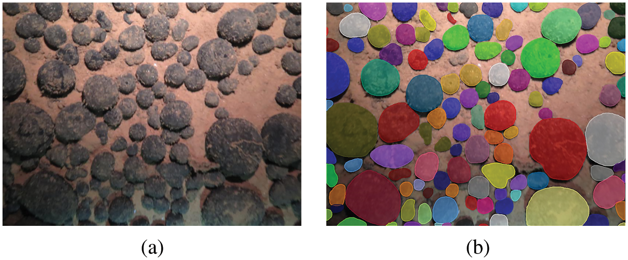
Figure 1: An example of deep-sea mineral image segmentation results. (a) Original image. (b) Image segmentation result
Due to the harsh working environment on the seafloor, there are many technical difficulties in the segmentation of deep-sea mineral images. First, the light sources of acquisition robots (i.e., autonomous underwater vehicles (AUVs) and remotely operated vehicles (ROVs)) are of various forms. Meanwhile, image capture is affected by light reflection, scattering, absorption, and attenuation due to the tendency of seawater to absorb suspended particulate matter [3]. Therefore, deep-sea imaging suffers from low contrast, overexposure, blurring, and color distortion. Second, some minerals may be obscured by mud and sand or marine organisms. In addition, pores may exist on the mineral surface, which makes it challenging to obtain the actual boundaries effectively. Finally, due to the complex type of seafloor geomorphology, seafloor minerals are attached to different topographies, which makes the distance between the deep towing system and minerals near and far, resulting in errors in laser scale imaging and difficulties in constructing a relationship model between the physical distance and the digital distance of the image, as shown in Fig. 2.
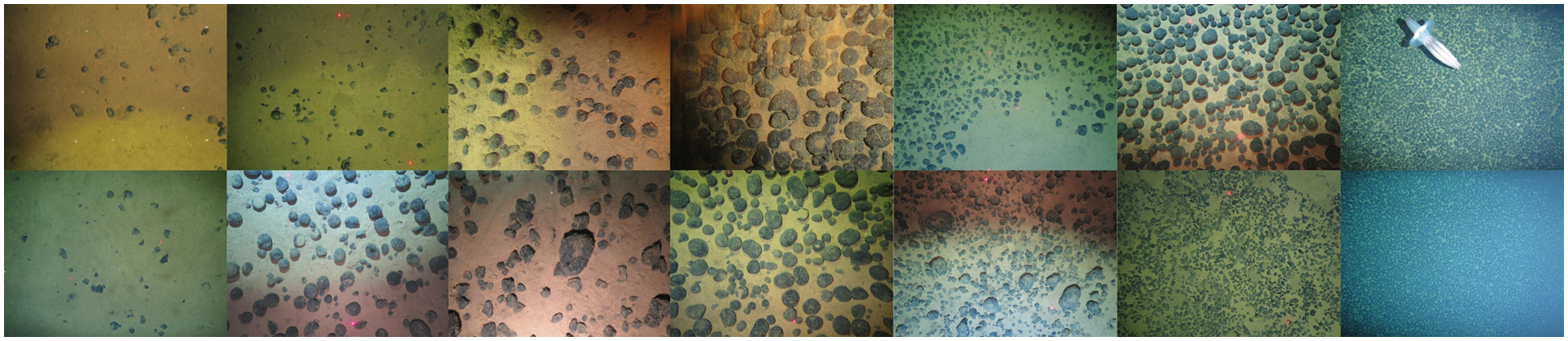
Figure 2: Images of seabed minerals under different areas, illuminations and depths
Several factors mentioned above make deep-sea mineral image segmentation difficult, and many natural image segmentation methods cannot be directly migrated to deep-sea nodule mineral image segmentation. At present, the research on deep-sea mineral image segmentation methods lags behind that of terrestrial mineral image segmentation. In this paper, a comprehensive description of representative deep-sea mineral image segmentation methods is given, traditional methods and deep learning methods for deep-sea nodule mineral image segmentation are compared and analyzed, and their performance and efficiency are discussed. Finally, the future trend of the development of deep-sea mineral image segmentation methods is foreseen.
2 Deep-Sea Nodule Mineral Segmentation Algorithm
Based on the current research on deep-sea nodule mineral image segmentation methods, this paper divides deep-sea mineral image segmentation algorithms into traditional segmentation methods and deep learning segmentation methods.
2.1 Traditional Segmentation Methods
2.1.1 Threshold-based Segmentation Methods
Threshold segmentation is the simplest image segmentation method, which divides the gray levels of an image into parts with one or more thresholds, considering pixels of the same gray level as belonging to the same class of objects [4]. Only a single threshold value is selected for deep-sea mineral images if the mineral type is not considered.
Park et al. [5] first segmented mineral images collected in the KODOS (Korean Deep Ocean Study) zone of the North Pacific Ocean by repeatedly performing contrast enhancement and median filtering to clarify the image edges and separated the minerals using threshold segmentation. Then, Park et al. [6] compensated for illumination by modeling depth information and grayscale variation, and then automatically classified the images into four categories, very sparse, sparse, medium, and dense based on the variance of the mineral images, and limited the threshold search range in the Otsu algorithm according to the nodule abundance. This method relies too much on the a priori characteristics of the image, does not generalize well, and is prone to under segmentation if the grayscale range spans a wide range.
Zhang et al. [7] proposed removing the pitch-black areas on both sides of the original image that could not be analyzed and processed to solve the illumination inhomogeneity problem. Then, the Niblack local binarization method was used instead of the global thresholding method to obtain the preliminary segmented images. Finally, the results were obtained by processing the pores within the mineral particles through morphological operations. However, this method directly discards the regions with poor brightness that will lose many details, and the choice of neighborhood size has a large impact on the Niblack thresholding segmentation results.
Schoening et al. [8] proposed the compact-morphology-based polymetallic nodule delineation (CoMoNoD) method, which dynamically determines thresholds based on heuristic ideas. In the image preprocessing stage, the contrast between nodule minerals and sediments is improved using median filtering, cubic difference scaling of the image, Gaussian filtering, and feature-space-based illumination and color enhancement (fSpice). In the segmentation stage, the image is converted into a grayscale image, and then a binary image is obtained by applying a compactness heuristic to determine the threshold dynamically; in the image postprocessing stage, by determining the nodule mineral centroid and using their convex hull to determine the contours, and finally ellipse fitting of the contours, the whole algorithm can achieve fast processing of deep-sea mineral images with GPU (graphics processing unit) boosting. This method shows comparable coverage results compared with three other clustering segmentation methods, PCCA [9], Rapid PCCA [10,11], and ES4C [12]. In contrast, CoMoNoD does not require training and runs the fastest, satisfying the requirement to complete quantitative analysis of nodule mineral abundance over several square kilometers within the cruise period. However, the algorithm is prone to misclassify other objects as nodule minerals, and the accuracy of resource assessment is limited.
Ma et al. [13] proposed using the MSR (multiscale retinex) enhancement algorithm for preprocessing. MSR [14] draws on the idea that the human visual system perceives the color and luminance of the target object to enhance the gray level of the RGB channel, thereby reducing the effect of color fading and making the image more consistent with human visual characteristics. The algorithm sets the ROI (region of interest) region for grayscale processing, uses bilateral filters to eliminate noise, equalizes the average image brightness by window histogram, and finally obtains the segmented image by window binarization. Window histogram equalization can effectively improve the global brightness of the image compared with global histogram equalization, and window binarization can obtain more details of the nodule boundary than global binarization. The segmentation results are more consistent with the morphological characteristics of the minerals.
Mao et al. [15] proposed a local threshold segmentation method based on the calculation of background gray values to solve the problem of morphological defects caused by factors such as uneven illumination and sediment coverage. Compared with the direct use of morphology to repair the object shape, this method repeatedly performs subtraction of the image background gray value and adjustment of the background gray value without the problem of disappearing the gap between nodule individuals and subsequent difficulty in segmenting them apart. However, the segmented morphology of nodule minerals can be distorted to some extent and does not correspond well to the actual nodule minerals morphology.
2.1.2 Clustering-based Segmentation Methods
Clustering is an algorithm that combines pixels with similar features such as texture, color, or grayscale values into the same class.
To solve the blurring problem arising from factors such as poor focus and sediment churning in deep-sea nodule mineral images. Zhang et al. [16] borrowed the idea of the image restoration technique [17] and argued that the seafloor light-sensitive intensity distribution is the essence of the degradation problem. The algorithm obtains an image of the seafloor light intensity distribution by fast Fourier transform and exponential filtering. It subtracts it from the original image by a certain percentage to eliminate the effect of distortion. After preprocessing, the nodule minerals are classified into three categories: bare nodules, shallowly buried nodules, and deeply buried nodules by clustering. The segmentation result is obtained by neighborhood filtering. This method can remove the interference caused by uneven illumination and enhance the sharpness of the image, increasing the contrast between the foreground and background.
To solve the problem of difficulty in establishing mapping relationships between feature vectors and classes directly, Schoening et al. [9] proposed the pixel-classification by cluster annotation (PCCA) based on hierarchical hyperbolic self-organizing map (H2SOM) [18], which introduces cluster prototypes based on the original mapping of feature vectors to classes to form a mapping of feature vectors to cluster prototypes and then to classes. The algorithm is divided into three stages. Gaussian filtering and histogram equalization are used in the first stage to correct the image brightness and contrast. In the second stage, unsupervised training is performed, and the color histogram of each pixel neighborhood is represented as a 48-dimensional feature vector. The feature vectors are mapped to 161 cluster prototypes by H2SOM. The feature vectors are mapped to the best-matching unit (BMU) using a beam search algorithm based on the Euclidean distance. Pattern recognition experts assigned 161 clusters to nodule minerals or backgrounds for image binarization. In the third stage, individual nodules were delineated by using blob detection and shape analysis. In terms of efficiency, the whole algorithm is inefficient, taking 3 s for image preprocessing, 3 s for feature extraction, and 18 s for H2SOM mapping, which makes this algorithm only available in the laboratory and does not meet the demand for real-time segmentation.
Schoening et al. [10,11] proposed Rapid PCCA by refactoring the PCCA code. It cuts the image into blocks that can be processed independently and places each block in GPU registers for parallel processing to achieve GPU acceleration in the fSpice color normalization, Gaussian filtering, feature extraction, and H2SOM mapping stages. In addition, parallel optimization improves CPU (central processing unit) and GPU utilization by refactoring the code to assign the three steps of preprocessing, H2SOM mapping, and postprocessing to three threads, which communicate through work queues. Cache efficiency has also been improved. These optimizations have reduced the time to rapidly segment a single image from 24 s to 0.3 s, making it possible to segment nodule mineral images on a research vessel.
Schoening et al. [12] proposed the evolutionary tuned segmentation using cluster co-occurrence and a convexity criterion (ES4C) to achieve fully automated image segmentation. The feature vector extraction and the H2SOM mapping in the ES4C algorithm are similar to the PCCA method, rather a compactness function is constructed, and the function value is maximized using a genetic algorithm. The compactness function combines the morphological compactness of the nodules and feature similarity in different parts of nodules to indicate the degree of segmentation quality. The algorithm applies to different datasets and clustering methods. However, the algorithm still has shortcomings. On the one hand, the heuristic algorithm implies that the optimal solution may not be found, and on the other hand, the compactness formula is prone to assign half of the clusters to a class, which can result in incorrect segmentation if multiple clusters form a single class of clustering results.
2.1.3 Spectral Information Based Segmentation Methods
Multispectral or hyperspectral images record the feedback information of spectral reflectance and spectral values of various objects under different bands of spectral irradiation. The segmentation algorithm based on spectral information uses the spectral features, spectral angles and other information of deep-sea mineral images at different wavelength bands to perform segmentation.
Sharma et al. [19] segmented deep-sea mineral images using ERDAS software, which provides a neural network-like approach. First, there is an unsupervised segmentation process where the algorithm assigns categories and gray levels to each pixel based on the similarity of the spectral features, and then the results are processed for supervised segmentation. In the supervised segmentation process, the expert creates polygonal selections around a portion of targets with typical features (e.g., manganese nodules and sediments), assigns different labels to different selections, merges targets belonging to the same category, and then chooses one of three algorithms, maximum likelihood (ML), Mahalanobis distance (MHD), or minimum distance (MD), to extend the type information of the labeled area of the image extrapolated to the unknown area of the whole image. The shortcomings of this method are that it requires an expert to create the category templates in the image. Furthermore, low-contrast regions and pixel-crossing regions are often not subdivided.
Dumke et al. [20] performed image segmentation on deep-sea hyperspectral image data by using two supervised classification methods, support vector machine (SVM) and spectral angle mapper (SAM) on ENVI software. The SVM takes the features of the target object as training samples and minimizes the empirical training error to achieve image segmentation. SAM performs the MNF transform on the spectral features to obtain spectral vectors by dimensionality reduction, matches them according to the reference spectra. Finally, it calculates the angle between the wave spectra to identify the feature regions and obtains the segmentation results. Both methods require labeled data for training, and the results show that SVM segmentation outperforms SAM since SVM allows for errors in training, thus improving generalization to unknown data. However, the segmentation results of both methods are poorly connected and are less effective for segmenting nodule minerals on the side of the back to the hyperspectral imager.
Lu et al. [21] used an improved active contour model to segment multispectral images of deep-sea nodule minerals at different wavelengths after noise reduction, smoothing, and erosion. It was demonstrated that this method could effectively segment low-contrast images. Among them, the spectrum at 650 nm wavelength performs the best. The whole algorithm does not require manual operation and can run in real-time on an ordinary computer.
2.2 Deep Learning Segmentation Methods
Convolutional neural networks (CNNs) [22] are the basis for which deep learning has achieved dominance in the image domain. It usually consists of four types of construction layers, convolutional (Conv), nonlinear, pooling, and fully connected (FC) layers. A loss function is used to calculate the model’s performance with specific weights by forward propagation on the training dataset. The weights are updated based on the loss values by backpropagation using a gradient descent optimization algorithm. A CNN is shown in Fig. 3. The Conv layer plays a key role in the CNN, consisting of many mathematical operations. The nonlinear layer, also called the activation layer, enhances the expressiveness of the model and enables it to learn more complex patterns. The classical activation functions [23] are sigmoid, tanh, ReLU, Leaky ReLU, etc. The function of the pooling layer is to remove the redundant part of the input features and reduce the size of the represented space to reduce the parameters and computation and control overfitting. The neurons in the fully connected layer are fully connected to all neurons in the previous layer, and it will finally spread them into a single vector that can be used as input for the next stage. Classical CNNs include LeNet [24], AlexNet [25], ZFNet [26], GoogLeNet [27], VGGNet [28] and ResNet [29].
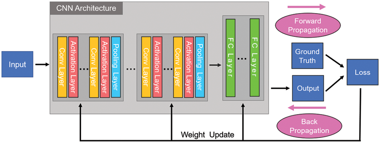
Figure 3: The architecture and training process of a CNN
Ciresan [30] started to use CNN to challenge the semantic segmentation task by using a sliding window approach, taking small image chunks (i.e., patches) centered on each pixel and feeding them into CNN to predict the semantic label. This approach breaks the precedent that CNN is only used for object classification. However, the disadvantage of this approach is that it needs to traverse each pixel point to extract patches for training and prediction, so it is time-consuming. Long et al. [31] proposed the fully convolutional network (FCN). The FC layer in the traditional CNN is replaced with a Conv layer to achieve end-to-end semantic segmentation. Compared with the traditional CNN, one replaces the FC with a Conv layer, allowing the model to derive scores for multiple input regions in a single forward calculation. Second, the FCN avoids the drawback that the input image size must be fixed in the FC layer and can handle inputs of arbitrary size. Third, after replacing the FC layer with the fully Conv layer, the output feature map is upsampled using deconvolution, so that the output prediction map and the input map have the same size. Ronneberger et al. [32] proposed a U-Net model based on CNN, which has achieved remarkable success in the field of biological image segmentation. The model does not require much data size for the training set, and the authors achieved good results using 30 images. The U-Net is also inspired by the FCN structure, which starts the upsampling after the Conv layer in stage 5, fuses the high-level and low-level features. Finally, the output prediction map is compared with the input map to calculate the loss of pixel semantic classification. U-Net is an encoder-decoder model, the first left half of the model is called the contracting path, which is a process of downsampling. The second right half is called the expanding path, which involves upsampling to expand the feature map. Finally, the feature map between each symmetric path is fused. However, the semantic segmentation models such as U-Net cannot solve the problem of segmenting different individuals of the same type of object. He et al. [33] proposed the Mask R-CNN instance segmentation model, which can solve the problem. It is a milestone in the R-CNN family of models, combining instance segmentation with Faster R-CNN and replacing ROI Pooling with ROI Align. The model achieves excellent results in instance segmentation, object detection, and keypoint detection tasks.
Song et al. [34] designed an improved segmentation algorithm based on the U-Net [32] network for deep-sea mineral images, in which the encoder part is consistent with the U-Net network and the decoder part is modified. In the decoder part, the features are fused by upsampling at different scales, and this method can identify more mineral particles and smooth the edges compared with U-Net.
Dong et al. [35] used Mask R-CNN for deep-sea nodule mineral image segmentation and compared it with three other deep learning segmentation networks U-Net [32], improved U-Net [34], and conditional generative adversarial network (CGAN) [36] on the same dataset. The results show that the segmentation effect of Mask R-CNN outperformed the other three networks with fewer missed objects.
3 Comparison of Deep-Sea Nodule Segmentation Algorithms
This section first describes the dataset of deep-sea nodule mineral images, introduces the evaluation metrics used for nodule mineral image segmentation methods, and finally compares these methods.
Due to the confidentiality of geological data and other reasons, many datasets are not publicly available. Most of the publicly available datasets do not have names and are only identified by the name of the research vessel and its voyage. Therefore, the datasets appearing in subsequent sections are replaced by the name and voyage of the research vessel. Tab. 1 lists the datasets used for the deep-sea nodule image segmentation.
(1) The R/V SONNE cruise SO205 [37] dataset was taken by the German research vessel SONNE in the German License Area (BGR) of the CCZ. The investigation focused on the formation of manganese nodules through microbial and abiotic early diagenetic processes. The filming was carried out with the OFOS, a towed underwater camera system that descends to approximately 2 m above the seafloor to take images. Since there is no light in the deep ocean, the light in the images is provided by a flash on the OFOS, with three laser pointers for calibration and a distance of 20 cm between each pair of laser points.
(2) The R/V SONNE cruise SO239 [38] dataset consists of 12 small datasets with a total of 198,322 images taken in four exploration contract areas of the CCZ (BGR, IOM, GSR, and IFREMER) and the Areas of Particular Environmental Interest (APEI) number 3. The International Seabed Authority (ISA) has defined nine APEI areas within the CCZ, intending to protect representative species and habitats within the CCZ. The scientific research studied the biodiversity and geochemical environment in the CCZ and examined the recovery time of benthic organisms after sediment changes.

(3) The R/V SONNE cruise SO242/1 [40] datasets consist of nine small datasets with a total of 190,697 seafloor images taken in the “disturbance and recolonization experimental” area (DEA) in the Peru Basin of the South Pacific Ocean. SO61 conducted a plow experiment in 1989 to simulate the environmental impacts of deep-sea mining of manganese nodules in this area. Between 1989 and 1997, SO64, SO70, and SO106 conducted several investigations to study the environmental impacts of the seafloor mechanical disturbance and to assess the extent of seafloor environmental recovery. SO242/1 resampled the DEA based on previous investigations to generate high-resolution bathymetric and optical maps for SO242/2.
(4) The R/V SONNE cruise SO242/2 [41] studied the recovery of ecosystem function and the state of re-equilibration of surface sediments in the experimental area after mechanical disturbance of the seafloor. SO242/2 consists of 20 small datasets with a total of 17,923 images of seafloor minerals.
(5) The R/V SONNE cruise SO268/1 + 2 [43] consists of 12 small datasets with a total of 41,088 seafloor images taken in the BGR and the Belgian license area (DEME). SO268 is designed to assess the environmental impacts of deep-sea mining of polymetallic nodules in the CCZ. The main goal is to study the potential long-term ecological impact of mining polymetallic manganese nodules on the CCZ.
(6) The RRS James Cook Cruise JC120 [45] dataset was taken during the first UK scientific cruise to the APEI area in the northeastern CCZ. The cruise was the first to sample benthic species and environments in the APEI area, and the survey acquired acoustic and visual image datasets using the Autosub6000 AUV, which was equipped with a variety of instrument modules. The survey also used the towed camera system HyBIS to provide detailed high-definition video and underwater photography. In addition, a large number of sediment samples, water samples, and biological samples were collected during the entire cruise.
(7) The 36th scientific research of Ocean Six used China’s self-developed 4500 m-class Seahorse ROV to obtain a large amount of comprehensive geophysical survey data from the contract area of the West Pacific seamount, collected much high-definition video data, and cobalt-rich crust samples.
3.2 Comparison of Evaluation Metrics and Different Methods
The evaluation metrics of the seabed mineral image segmentation methods can be divided into the following three aspects by compiling the existing literature: time-based evaluation metrics, segmentation degree-based evaluation metrics, and pixel-based evaluation metrics.
Before introducing the evaluation metrics of deep-sea mineral image segmentation specifically, several segmentation cases are introduced: true positive (TP) indicates pixels that determine minerals as foreground (minerals); false negative (FN) indicates pixels that minerals are incorrectly determined as background (nonmineral); false positive (FP) indicates pixels that incorrectly segment background as foreground; and true negative (TN) indicates pixels that correctly segment background as background, as shown in Fig. 4.
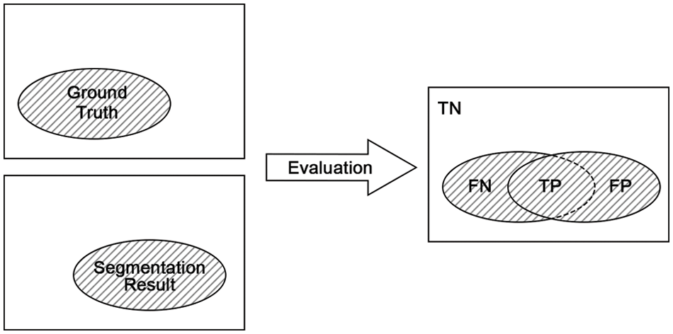
Figure 4: Schematic representation of the meaning of TP, TN, FP and FN
3.2.1 Time-based Evaluation Metrics
The easiest and most effective way to evaluate different segmentation methods is to compare their running speed, i.e., the speed can be quantified by time, which can be divided into training (if needed), preprocessing, segmentation, and postprocessing time, and we use the term “time” uniformly here.
3.2.2 Segmented Degree Based Evaluation Metrics
Some nodule mineral image segmentation methods do not directly use evaluation metrics but use the Coverage and Abundance in the mineral evaluation to support the accuracy of the segmentation. The Coverage refers to the coverage area of nodules in a specific area of the seafloor surface. The Abundance is the weight of polymetallic nodules per square meter area.
Compactness is used to measure the correlation between cluster objects, and it is a metric to evaluate the regularity of the shape, area size, compactness and smoothness of the segmented boundary of each segmented region. It is an unsupervised evaluation performed by directly computing the feature parameters of the resulting image without relying on the reference image.
3.2.3 Pixel-based Evaluation Metrics
The Intersection over Union (IoU) [31]/Jaccard Index (JI) is a commonly used evaluation metric in image segmentation, which refers to the ratio of the intersection of two sets
Accuracy [30] refers to the percentage of correctly predicted pixel results to the total sample pixels, assuming Total Samples is the total image space,
Precision [46] is the proportion of pixels predicted to be minerals that are actually minerals. It can be calculated using Eq. (3).
Sensitivity/Recall/True Positive Rate (TPR) [46], which refers to the proportion of pixels that are actually minerals that are predicted to be correct, the Sensitivity formula is given in Eq. (4).
Specificity/True Negative Rate (TNR) refers to the proportion of actual nonmineral pixels that are correctly predicted, and the Specificity calculated using Eq. (5).
We summarize the abovementioned deep-sea nodule mineral segmentation methods in Tab. 2. The threshold segmentation method can be effective when the grayscale difference between the foreground and background is large, and it directly uses the grayscale characteristics of the image, so it is computationally simple, more efficient, and faster. However, it is sensitive to noise, and the segmentation effect is average when the grayscale difference is not obvious or different object grayscale values have overlap, so a combination of other methods is needed. A suitable threshold value is also the key to threshold segmentation. Clustered segmentation is suitable for situations where uncertainty and ambiguity exist in the image and is easily affected by the initial parameters, so manual intervention is required to initialize the parameters to approach the global optimal solution and improve the segmentation speed. In addition, it takes little account of spatial information and is more sensitive to noise and inhomogeneity of grayscale variations.

The spectral segmentation method utilizes the multidimensional spectral information of the image, which has high spatial correlation and rich texture details, but its processing data volume is large and slow, and the segmentation accuracy is low. The deep learning approach can suppress noise and better recover the natural form of minerals, but their model structure is complex and requires a large amount of data training, and the segmentation accuracy is related to the amount of data. Semantic segmentation cannot distinguish different instances of the same class, while instance segmentation can. Instance segmentation models tend to be more complex and slightly slower than semantic segmentation models, but their segmentation performance is better. We use different deep learning models to segment the seabed images, and the visualization results are shown in Fig. 5.
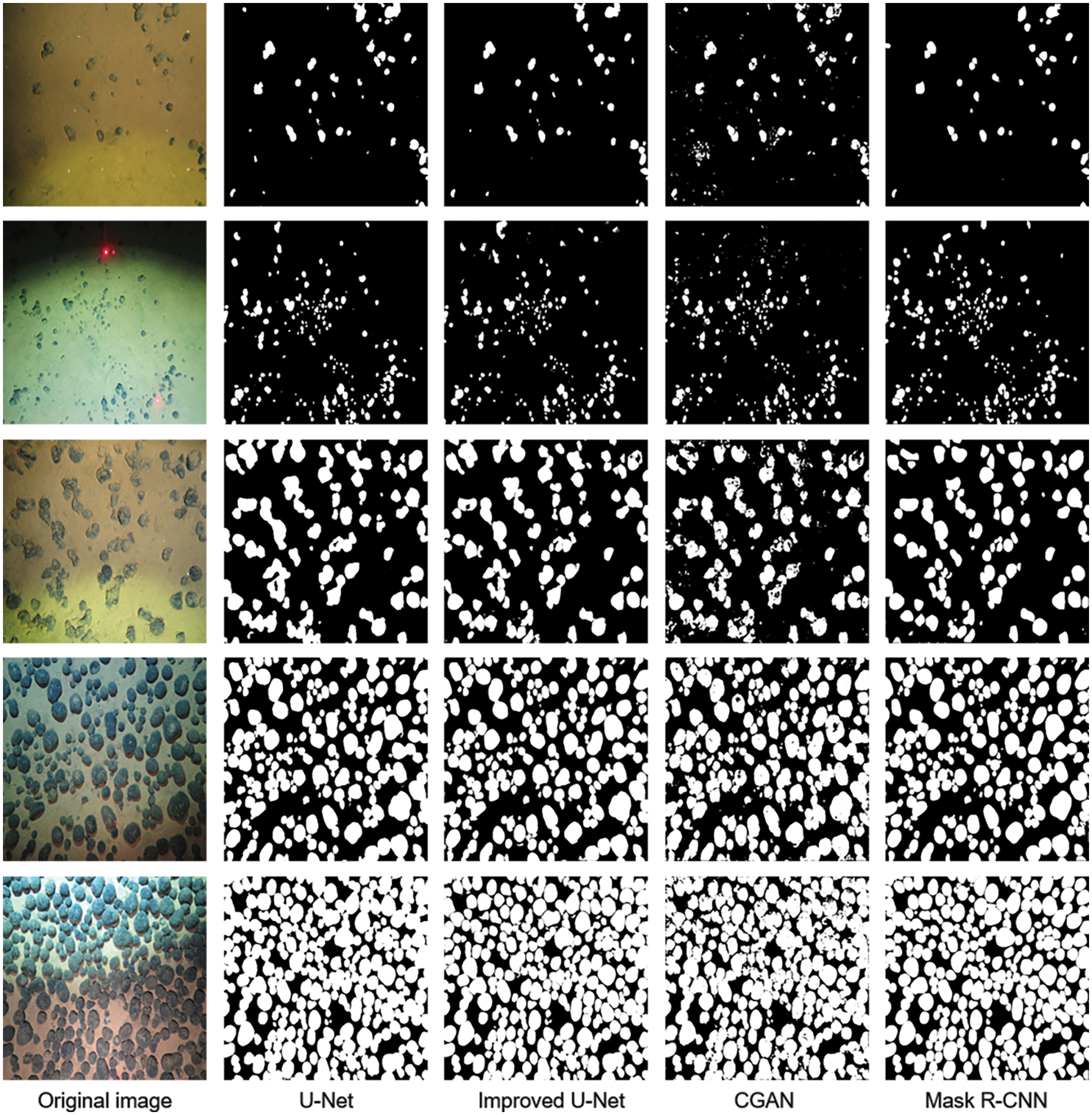
Figure 5: Comparison of visualization results of deep learning methods for mineral image segmentation
4 Future Research Methods and Open Questions
4.1 Establishing a Public Dataset of Deep-sea Mineral Images
Most deep-sea nodule image datasets are not publicly available due to the expensive acquisition of deep-sea nodule images and the high confidentiality of geographic information. The publicly available datasets contain only nodule minerals with specific characteristics, so there is a need to build a deep-sea mineral image dataset that provides deep-sea mineral images with different sea areas, depths, abundances, and brightnesses. In addition, as the 3D image segmentation model becomes increasingly mature, the segmentation of deep-sea mineral images also needs to establish a complete 3D image dataset.
4.2 Improvement of the Segmentation Model Based on Deep Learning
In recent years, image segmentation algorithms based on deep learning have achieved results better than traditional segmentation algorithms and have excellent prospects to develop. Among them, the Mask R-CNN model has achieved great results for deep-sea mineral image segmentation. However, balancing segmentation accuracy and real-time is still a long way from industrial applications. To improve the speed of the segmentation algorithm, many recent studies have improved segmentation models from some new aspects, such as the anchor-free instance segmentation algorithm FAPIS [47] with the abandonment of generating anchor and YOLACT++ [48] with the abandonment of feature localization. Future research should considers applying these models for deep-sea nodule mineral image segmentation to assist in real-time assessment of deep-sea nodule mineral resources to help explore and research the deep ocean.
Nodule minerals in the deep sea show a wide variety of obscuring structures. Some nodule minerals are partially or entirely covered by sediment, while some are covered by flora and fauna. Organisms such as sponges, aphids, octopuses, and soft corals obscure the nodule edges’ high-frequency information and increase segmentation difficulty. We can learn from the methods of object segmentation for obscured objects in other fields. Rizon et al. [49] used texture analysis and the Hough transform to identify the objects and performed ellipse fitting and centering location. Zhan et al. [50] proposed a framework for self-supervised scene de-occlusion with some effectiveness. Moreover, for the case of semitransparent biological occlusion, an image defogging algorithm can be used to reduce the impact caused by the occlusion before further segmentation. Inspired by contrast learning, Wu et al. [51] proposed a contrast regularization mechanism combined with an autoencoder network, which showed some effectiveness in image defogging.
4.4 Subpixel Level Segmentation
With the increasing requirement of segmentation accuracy in deep-sea resource assessment, pixel-level segmentation can hardly meet the needs of actual accurate resource assessment. The subpixel-level segmentation method should also be applied to deep-sea nodule mineral images. There exist pixels between two pixels on the imaging surface, i.e., subpixels, which are affected by the hardware system, only lacking a more accurate sensor to detect them, as shown in Fig. 6. A feasible way to address the subpixels is to approximate them using interpolation, which will give a more accurate segmentation result.
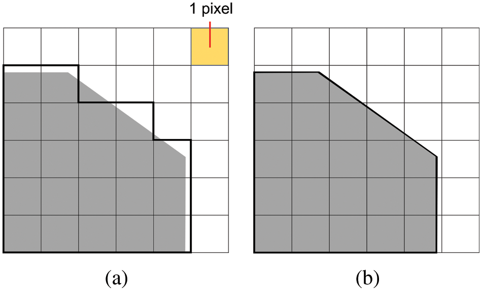
Figure 6: (a) Pixel-level segmentation. (b) Subpixel-level segmentation
4.5 Combination of Multiple Segmentation Methods
Traditional image segmentation methods based on artificial cognitive drive are not end-to-end processing and require more complex image preprocessing. However, traditional segmentation methods also have advantages, such as better maturity, speed, less code, and great interpretability. Data-driven deep learning methods have the following limitations. First, the results are not fully controllable. CNNs often have hundreds of convolutional layers, and the total number of automatically learned parameters can reach millions. Second, it easily leads to overfitting, and generalization is challenging in different seas. Third, image annotation is very costly. The manual annotation workload depends on the number of objects in each image, the object species, and the resolution of individual images. In addition, as the labellers have different knowledge about the geological structure of the deep sea, different labellers will mark the same object with different labels [52]. Fourth, the segmentation effect of small objects is not good, and when the original image is downsampled several times, the extracted feature map will disappear. Fifth, the computer computing power, memory capacity and energy consumption requirements are high.
To solve these problems, one idea is to fuse traditional and deep learning methods, use deep learning methods to adjust the results of traditional segmentation methods, and use traditional segmentation methods to increase the recall of deep learning results. Bringing out the advantage of the nonlinear structure of neural networks in deep learning that can fit complex higher-order nonlinear relationships in degenerate models, the results of traditional segmentation methods are adjusted using deep learning models. In turn, the results of traditional segmentation methods are used to complement the recall of deep learning results.
4.6 Interpretability of Deep Learning Models
Recent papers have shown that deep learning-based image segmentation methods perform better than traditional methods in terms of accuracy, generalization, and robustness. Deep learning-based segmentation methods often do not require morphological operations to fill the interior of minerals and do not generate much noise. However, deep learning-based methods suffer from the problem that the model is difficult to interpret, i.e., it is difficult to interpret the meaning of the parameters in the middle layers of the model, leading researchers to often rely only on experience to optimize the neural network. Currently, more commonly used methods use a combination of different model frameworks and components to improve model performance. For example, attention mechanisms [53,54], residual networks [29,55,56], hidden layer analysis methods [26,57], prior knowledge [58,59], simulation model methods [60], and transformers [61,62], etc. are added to the original framework to test their rise points for evaluation metrics. Most of these methods obtain the rise points and then return to analyze the principles behind the network. Establishing a perfect mechanism to improve the interpretability of the model is the future direction to be considered and studied.
Deep-sea nodule minerals are a particular class of objects in computer vision, and whether they can be segmented correctly is the key to achieving mineral evaluation. At present, there has been some progress in research on deep-sea mineral image segmentation. However, limited by the seafloor environment, nodule minerals themselves, and the diversity of mineral forms in different seas, so the features extracted in one sea are often inconsistent with those in another. In addition, problems such as occlusion and real-time have not been fundamentally solved.
This paper provides a comprehensive description of deep-sea nodule mineral image segmentation methods, including traditional and deep learning-based mineral segmentation methods. We emphasize algorithms, datasets and evaluation metrics and summarize the classes to which different segmentation methods belong and their important features. The traditional image segmentation methods are slightly less effective and rely on expertise and experience. Deep learning methods have improved in terms of robustness, accuracy and generalization, but further improvements are needed in terms of interpretability, hardware requirements and real-time performance, and the accuracy of its segmentation results still does not meet the requirements in practical deep-sea resource assessment. Finally, we discuss the future challenges and development directions of image segmentation of deep-sea nodule minerals. We believe that combining multiple segmentation methods and utilizing multidomain knowledge is a key point to be explored in solving the bottleneck that currently exists, which is also our current work in progress. We hope that this paper will provide a quick introduction for newcomers to the field and inspiration for related researchers.
Acknowledgement: Thanks to other students in the Media Computing Laboratory of the Minzu University of China and anonymous reviewers for their valuable comments and contributions to this research.
Funding Statement: This work was supported in part by the National Science Foundation Project of P.R. China under Grant No.52071349, No.U1906234, partially supported by the Open Project Program of Key Laboratory ofMarine Environmental Survey Technology and Application, Ministry of Natural Resource MESTA-2020-B001, Young and Middle-aged Talents Project of the State Ethnic Affairs Commission, the Crossdisciplinary Research Project of Minzu University of China (2020MDJC08), and the Graduate Research and Practice Projects of Minzu University of China (SZKY2021039).
Conflicts of Interest: The authors declare that they have no conflicts of interest to report regarding the present study.
1. M. Lodge, “Deep sea mining: The new resource frontier?,” in Outlook on the Global Agenda 2015, Cologny, Geneva, Switzerland: World Economic Forum, pp. 73–74, 2015. [Online]. Available: https://www.weforum.org/reports/outlook-global-agenda-2015 [Accessed Jan. 12, 2022]. [Google Scholar]
2. J. R. Hein, K. Mizell, A. Koschinsky and T. A. Conrad, “Deep-ocean mineral deposits as a source of critical metals for high and green-technology applications: Comparison with land-based resources,” Ore Geology Reviews, vol. 51, pp. 1–14, 2013. [Google Scholar]
3. D. Kyryliuk and S. Kratzer, “Summer distribution of total suspended matter across the baltic sea,” Frontiers in Marine Science, vol. 5, pp. 504, 2019. [Google Scholar]
4. S. Mahajan, N. Mittal and A. K. Pandit, “Image segmentation using multilevel thresholding based on type II fuzzy entropy and marine predators algorithm,” Multimedia Tools and Applications, vol. 80, no. 13, pp. 19335–19359, 2021. [Google Scholar]
5. C. Y. Park, H. T. Chon and J. K. Kang, “Correction of nodule abundance using image analysis technique on manganese nodule deposits,” Economic and Environmental Geology, vol. 29, no. 4, pp. 429–437, 1996. [Google Scholar]
6. C. Y. Park, S. H. Park and C. W. Kim, “An image analysis technique for exploration of manganese nodules,” Marine Georesources and Geotechnology, vol. 17, no. 4, pp. 371–386, 1999. [Google Scholar]
7. D. X. Zhang, B. Li, M. J. Li, L. L. Qiu and H. D. Zhao, “Camera system in deep sea and image processing system for seabed mineral resources (In Chinese),” Science Technology and Engineering, vol. 16, no. 34, pp. 1671–1815. 2016. [Google Scholar]
8. T. Schoening, D. O. B. Jones and J. Greinert, “Compact-morphology-based poly-metallic nodule delineation,” Scientific Reports, vol. 7, no. 1, pp. 1–12, 2017. [Google Scholar]
9. T. Schoening, “Automated detection in benthic images for megafauna classification and marine resource exploration: Supervised and unsupervised methods for classification and regression tasks in benthic images with efficient integration of expert knowledge,” Ph.D. dissertation, Bielefeld University, Germany, 2015. [Google Scholar]
10. T. Schoening, D. Langenkämper, B. Steinbrink, D. Brün and T. W. Nattkemper, “Rapid image processing and classification in underwater exploration using advanced high performance computing,” in 2015 MTS/IEEE OCEANS, Washington, DC, USA, pp. 1–4, 2015. [Google Scholar]
11. T. Schoening, B. Steinbrink, D. Brün, T. Kuhn and T. W. Nattkemper, “Ultra-fast segmentation and quantification of poly-metallic nodule coverage in high-resolution digital images,” in Proc. of the 2013 42th Underwater Mining Institute (UMI), Rio de Janeiro and Porto de Galinhas, Brazil, pp. 1–10, 2013. [Google Scholar]
12. T. Schoening, T. Kuhn, D. O. B. Jones, E. Simon-Lledo and T. W. Nattkemper, “Fully automated image segmentation for benthic resource assessment of poly-metallic nodules,” Methods in Oceanography, vol. 15, pp. 78–89, 2016. [Google Scholar]
13. X. L. Ma, Z. W. He, J. Y. Huang, Y. H. Dong and C. F. You, “An automatic analysis method for seabed mineral resources based on image brightness equalization,” in Proc. of the 2019 3th Int. Conf. on Digital Signal Processing (ICDSP), Jeju Island, South Korea, pp. 32–37, 2019. [Google Scholar]
14. S. Zhang, T. Wang, J. Y. Dong and H. Yu, “Underwater image enhancement via extended multi-scale retinex,” Neurocomputing, vol. 245, pp. 1–9, 2017. [Google Scholar]
15. H. D. Mao, Y. L. Liu, H. Z. Yan, C. Qian and J. Xue, “Image processing of manganese nodules based on background gray value calculation,” Computers, Materials & Continua, vol. 65, no. 1, pp. 511–527, 2020. [Google Scholar]
16. Y. J. Zhang and J. W. Shi, “A study of image reconstruction and image processing techniques for photos of deep-sea polymetallic nodules (In Chinese),” Geophysical and Geochemical Exploration, vol. 13, no. 6, pp. 435–441, 1989. [Google Scholar]
17. M. Cannon, A. Lehar and F. Preston, “Background pattern removal by power spectral filtering,” Applied Optics, vol. 22, no. 6, pp. 777–779, 1983. [Google Scholar]
18. J. Ontrup and H. Ritter, “A hierarchically growing hyperbolic self-organizing map for rapid structuring of large data sets,” in Proc. of the 2005 5th Workshop on Self-Organizing Maps (WSOM), Paris, France, pp. 471–478, 2005. [Google Scholar]
19. R. Sharma, S. J. Sankar, S. Samanta, A. A. Sardar and D. Gracious, “Image analysis of seafloor photographs for estimation of deep-sea minerals,” Geo-Marine Letters, vol. 30, no. 6, pp. 617–626, 2010. [Google Scholar]
20. I. Dumke, S. M. Nornes, A. Purser, Y. Marcon, M. Ludvigsen et al., “First hyperspectral imaging survey of the deep seafloor: High-resolution mapping of manganese nodules,” Remote Sensing of Environment, vol. 209, pp. 19–30, 2018. [Google Scholar]
21. H. M. Lu, Y. Q. Zheng, K. Hatanom, Y. J. Li, S. Nakashima et al., “Hyperspectral images segmentation using active contour model for underwater mineral detection,” in 2018 3th Int. Symp. on Artificial Intelligence and Robotics (ISAIR), Nanjing, China, pp. 513–522, 2018. [Google Scholar]
22. Y. Lecun and Y. Bengio, “Convolutional networks for images, speech, and time series,” in The Handbook of Brain Theory and Neural Networks, Cambridge, MA, USA: MIT Press, pp. 255–258, 1998. [Google Scholar]
23. C. E. Nwankpa, W. Ijomah, A. Gachagan and S. Marshall, “Activation functions: Comparison of trends in practice and research for deep learning,” arXiv preprint arXiv: 1811.03378v1, pp. 1–20, 2018. [Google Scholar]
24. Y. Lecun, L. Bottou, Y. Bengio and P. Haffner, “Gradient-based learning applied to document recognition,” Proc. of the IEEE, vol. 86, no. 11, pp. 2278–2324, 1998. [Google Scholar]
25. A. Krizhevsky, I. Sutskever and G. E. Hinton, “ImageNet classification with deep convolutional neural networks,” in 2012 Advances in Neural Information Processing Systems (NIPS), Lake Tahoe, NV, USA, vol. 25, pp. 1097–1105, 2012. [Google Scholar]
26. M. D. Zeiler and R. Fergus, “Visualizing and understanding convolutional networks,” in Proc. of the 2014 European Conf. on Computer Vision (ECCV), Zurich, Switzerland, pp. 818–833, 2014. [Google Scholar]
27. C. Szegedy, W. Liu, Y. Q. Jia, P. Sermanet, S. Reed et al., “Going deeper with convolutions,” in Proc. of the 2015 IEEE Int. Conf. on Computer Vision and Pattern Recognition (CVPR), Boston, MA, USA, pp. 1–9, 2015. [Google Scholar]
28. K. Simonyan, and A. Zisserman, “Very deep convolutional networks for large-scale image recognition,” in 2015 3th Int. Conf. on Learning Representations (ICLR), San Diego, CA, USA, pp. 1–14, 2015. [Google Scholar]
29. K. M. He, X. Y. Zhang, S. Q. Ren and J. Sun, “Deep residual learning for image recognition,” in Proc. of the 2016 IEEE Int. Conf. on Computer Vision and Pattern Recognition (CVPR), Las Vegas, NV, USA, pp. 770–778, 2016. [Google Scholar]
30. D. Ciresan, A. Giusti, L. Gambardella and J. Schmidhuber, “Deep neural networks segment neuronal membranes in electron microscopy images,” in Proc. of the 2012 25th Advances in Neural Information Processing Systems (NIPS), Lake Tahoe, NV, pp. 2843–2851, 2012. [Google Scholar]
31. J. Long, E. Shelhamer and T. Darrell, “Fully convolutional networks for semantic segmentation,” in Proc. of the 2015 IEEE Int. Conf. on Computer Vision and Pattern Recognition (CVPR), Boston, MA, USA, pp. 3431–3440, 2015. [Google Scholar]
32. O. Ronneberger, P. Fischer and T. Brox, “U-Net: Convolutional networks for biomedical image segmentation,” in 2015 18th Int. Conf. on Medical Image Computing and Computer Assisted Intervention (MICCAI), Munich, Germany, pp. 1–8, 2015. [Google Scholar]
33. K. M. He, G. Gkioxari, P. Dollár and R. Girshick, “Mask R-CNN,” in Proc. of the 2017 IEEE Int. Conf. on Computer Vision and Pattern Recognition (CVPR), Honolulu, HI, USA, pp. 2961–2969, 2017. [Google Scholar]
34. W. Song, N., Zheng, X. C. Liu, L. R. Qiu and R. Zheng, “An improved U-net convolutional networks for seabed mineral image segmentation,” IEEE Access, vol. 7, pp. 82744–82752, 2019. [Google Scholar]
35. L. H. Dong, H. L. Wang, W. Song, J. X. Xia and T. M. Liu, “Deep sea nodule mineral image segmentation algorithm based on mask R-CNN,” in 2021 4th ACM Turing Award Celebration Conf. (ACM TURC), Hefei, China, pp. 278–284, 2021. [Google Scholar]
36. M. Mirza and S. Osindero, “Conditional generative adversarial nets,” arXiv preprint arXiv: 1411.1784v1, pp. 1–7, 2014. [Google Scholar]
37. C. Rühlemann, L. Baumann, M. Blöthe, A. Bruns, A. Eisenhauer et al., Cruise Report SO-205 Mangan—Microbiology, Paleoceanography and Biodiversity in the Manganese Nodule Belt of the Equatorial NE Pacific—Papeete, Tahiti-Manzanillo, Mexico, 14 April—21 may 2010, Hannover, Germany: Bundesanstalt für Geowissenschaften und Rohstoffe, pp. 1–114, 2010. [Google Scholar]
38. P. M. Arbizu and M. Haeckel, RV SONNE Fahrtbericht/Cruise Report SO239: EcoResponse Assessing the Ecology, Connectivity and Resilience of Polymetallic Nodule Field Systems, Balboa (Panama)–Manzanillo (Mexico) 11.03.-30.04. 2015, Kiel, Germany: Helmholtz-Zentrum für Ozeanforschung, pp. 1–204, 2015. [Google Scholar]
39. J. Greinert, T. Schoening, K. Köser and M. Rothenbeck, “Seafloor images and raw context data along AUV tracks during SONNE cruises SO239 and SO242/1,” in Pangaea Data, Germany, Pangaea, 2017. [Online]. Available: https://doi.pangaea.de/10.1594/PANGAEA.882349. [Accessed Jan. 12, 2022]. [Google Scholar]
40. J. Greinert, RV Sonne Fahrtbericht/Cruise Report SO242-1: JPI OCEANS Ecological Aspects of Deep-Sea Mining, DISCOL Revisited, Guayaquil—Guayaquil (Equador28.07.-25.08.2015, Kiel, Germany: Helmholtz-Zentrum für Ozeanforschung, pp. 1–290, 2015. [Google Scholar]
41. A. Boetius, RV SONNE Fahrtbericht/Cruise Report SO242-2 [SO242/2]: JPI OCEANS Ecological Aspects of Deep-Sea Mining, DISCOL Revisited, Guayaquil - Guayaquil (Equador28.08.-01.10.2015, Kiel, Germany: Helmholtz-Zentrum für Ozeanforschung, pp. 1–552, 2015. [Google Scholar]
42. A. Purser, Y. Marcon and A. Boetius, “Seafloor images from the Peru Basin Disturbance and Colonization (DISCOL) area collected during SO242/2,” in Pangaea Data, Germany, Pangaea, 2018. [Online]. Available: https://doi.pangaea.de/10.1594/PANGAEA.890634. [Accessed Jan. 12, 2022]. [Google Scholar]
43. P. Linke and M. Haeechel, Short Cruise Report RV SONNE SO268/1 + 2, Manzanillo–Manzanillo–Vancouver, 17.02.2019 – 27.05.2019, Kiel, Germany: Helmholtz-Zentrum für Ozeanforschung, pp. 1–20, 2015. [Google Scholar]
44. A. Purser, Y. Bodur, S. Ramalo and T. Stratmann, “Seafloor images of undisturbed and disturbed polymetallic nodule province seafloor collected during RV SONNE expeditions SO268/1 + 2,” in Pangaea Data, Germany, Pangaea, 2021. [Online]. Available: https://doi.pangaea.de/10.1594/PANGAEA.935856. [Accessed Jan. 12, 2022]. [Google Scholar]
45. D. O. B. Jones, RRS James Cook Cruise JC120 15 Apr-19 may 2015. Manzanillo to Manzanillo, Mexico. Managing Impacts of Deep-sea Resource Exploitation (MIDASClarion-Clipperton Zone North Eastern Area of Particular Environmental Interest, Southampton, UK: National Oceanography Centre, pp. 1–117, 2015. [Google Scholar]
46. Y. Tan, L. Tan, X. Y. Xiang, H. Tang, J. H. Qin et al., “Automatic detection of aortic dissection based on morphology and deep learning,” Computers, Materials & Continua, vol. 62, no. 3, pp. 1201–1215, 2020. [Google Scholar]
47. K. Nguyen and S. Todorovic, “FAPIS: A Few-shot anchor-free part-based instance segmenter,” in Proc. of the 2021 IEEE/CVF Int. Conf. on Computer Vision and Pattern Recognition (CVPR), Nashville, TN, USA, pp. 11099–11108, 2021. [Google Scholar]
48. D. Bolya, C. Zhou, F. Y. Xiao and Y. J. Lee, “Yolact++: Better real-time instance segmentation,” in Proc. of the 2019 IEEE/CVF Int. Conf. on Computer Vision (ICCV), Seoul, South Korean, pp. 9157–9166, 2019. [Google Scholar]
49. M. Rizon, N. A. N. Yusri, M. F. A. Kadir, A. R. Mamat, A. Z. A. Aziz et al., “Determination of mango fruit from binary image using randomized hough transform,” in 2015 8th Int. Conf. on Machine Vision (ICMV), Barcelona, Spain, vol. 9875, pp. 9–13, 2015. [Google Scholar]
50. X. H. Zhan, X. G. Pan, B. Dai, Z. W. Liu, D. H. Lin et al., “Self-supervised scene de-occlusion,” in Proc. of the 2020 IEEE/CVF Int. Conf. on Computer Vision and Pattern Recognition (CVPR), Seattle, WA, USA, pp. 3784–3792, 2020. [Google Scholar]
51. H. Y. Wu, Y. Y. Qu, S. H. Lin, J. Zhou, R. Z. Qiao et al., “Contrastive learning for compact single image dehazing,” in Proc. of the 2021 IEEE/CVF Int. Conf. on Computer Vision and Pattern Recognition (CVPR), Nashville, TN, USA, pp. 10551–10560, 2021. [Google Scholar]
52. J. M. Durden, B. J. Bett, T. Schoening, K. J. Morris, T. W. Nattkemper et al., “Comparison of image annotation data generated by multiple investigators for benthic ecology,” Marine Ecology Progress Series, vol. 552, pp. 61–70, 2016. [Google Scholar]
53. Y. Y. Liu, S. Zhang, H. Y. Yue, Y. Y. Wang, Y. H. Feng et al., “Straw segmentation algorithm based on modified UNet in complex farmland environment,” Computers, Materials & Continua, vol. 66, no. 1, pp. 247–262, 2021. [Google Scholar]
54. G. Hou, J. Qin, X. Xiang, Y. Tan and N. N. Xiong, “AF-Net: A medical image segmentation network based on attention mechanism and feature fusion,” Computers, Materials & Continua, vol. 69, no. 2, pp. 1877–1891, 2021. [Google Scholar]
55. J. Tahir, S. R. Naqvi, K. Aurangzeb and M. Alhussein, “A saliency based image fusion framework for skin lesion segmentation and classification,” Computers, Materials & Continua, vol. 70, no. 2, pp. 3235–3250, 2022. [Google Scholar]
56. S. Mahajan, A. Raina, X. Z. Gao and A. K. Pandit, “COVID-19 detection using hybrid deep learning model in chest x-rays images,” Concurrency and Computation-Practice and Experience, vol. 34, no. 5, pp. e6747, 2022. [Google Scholar]
57. W. Samek, A. Binder, G. Montavon, S. Bach and K. Robert, “Evaluating the visualization of what a deep neural network has learned,” IEEE Transactions on Neural Networks and Learning Systems, vol. 28, no. 11, pp. 2660–2673, 2016. [Google Scholar]
58. W. C. Kuo, A. Angelova, J. Malik and T. Y. Lin, “Shapemask: Learning to segment novel objects by refining shape priors,” in Proc. of the 2019 IEEE/CVF Int. Conf. on Computer Vision (ICCV), Seoul, South Korean, pp. 9207–9216, 2019. [Google Scholar]
59. K. Khan, R. U. Khan, J. Ali, I. Uddin, S. Khan et al., “Race classification using deep learning,”, Computers, Materials & Continua, vol. 68, no. 3, pp. 3483–3498, 2021. [Google Scholar]
60. B. J. Hou and Z. H. Zhou, “Learning with interpretable structure from gated RNN,” IEEE Transactions on Neural Networks and Learning Systems, vol. 31, no. 7, pp. 2267–2279, 2020. [Google Scholar]
61. Z. L. Deng, B. Zhou, P. He, J. F. Huang, O. Alfarraj et al., “A Position-aware transformer for image captioning,” Computers, Materials & Continua, vol. 70, no. 1, pp. 2065–2081, 2021. [Google Scholar]
62. G. N. Chandrika, K. Alnowibet, K. S. Kautish, E. S. Reddy, A. F. Alrasheedi et al., “Graph transformer for communities detection in social networks,” Computers, Materials & Continua, vol. 70, no. 3, pp. 5707–5720, 2022. [Google Scholar]
 | This work is licensed under a Creative Commons Attribution 4.0 International License, which permits unrestricted use, distribution, and reproduction in any medium, provided the original work is properly cited. |