DOI:10.32604/cmc.2022.027345
| Computers, Materials & Continua DOI:10.32604/cmc.2022.027345 | |
| Article |
An Efficient Ensemble Model for Various Scale Medical Data
Information System Department, Faculty of Computers and Information, Mansoura University, Mansoura, 35516, Egypt
*Corresponding Author: Heba A. Elzeheiry. Email: hebaaly@mans.edu.eg
Received: 15 January 2022; Accepted: 12 April 2022
Abstract: Electronic Health Records (EHRs) are the digital form of patients’ medical reports or records. EHRs facilitate advanced analytics and aid in better decision-making for clinical data. Medical data are very complicated and using one classification algorithm to reach good results is difficult. For this reason, we use a combination of classification techniques to reach an efficient and accurate classification model. This model combination is called the Ensemble model. We need to predict new medical data with a high accuracy value in a small processing time. We propose a new ensemble model MDRL which is efficient with different datasets. The MDRL gives the highest accuracy value. It saves the processing time instead of processing four different algorithms sequentially; it executes the four algorithms in parallel. We implement five different algorithms on five variant datasets which are Heart Disease, Health General, Diabetes, Heart Attack, and Covid-19 Datasets. The four algorithms are Random Forest (RF), Decision Tree (DT), Logistic Regression (LR), and Multi-layer Perceptron (MLP). In addition to MDRL (our proposed ensemble model) which includes MLP, DT, RF, and LR together. From our experiments, we conclude that our ensemble model has the best accuracy value for most datasets. We reach that the combination of the Correlation Feature Selection (CFS) algorithm and our ensemble model is the best for giving the highest accuracy value. The accuracy values for our ensemble model based on CFS are 98.86, 97.96, 100, 99.33, and 99.37 for heart disease, health general, Covid-19, heart attack, and diabetes datasets respectively.
Keywords: Electronic health records (EHRs); Random forest (RF); Decision tree (DT); linear model (LR); Multi-layer Perceptron (MLP); MDRL; correlation feature selection (CFS)
EHRs make medical data available for authorized uses. It contains patient’s reports, history, diagnoses, x-rays, and medications. The developed medical approaches in critical care field make the patients protected from future critical situations. Several infections, such as pneumonia, bloodstream infection, and catheter-associated urinary tract infections, may be associated with persistent devices used in intensive care units (ICUs). Infections due to previous procedures undertaken are also possible, such as surgical site infection. All of the previous collected data from different sources and in different structures forms what is called medical data. Searching for medical information without a classification is the same as searching for a needle in a haystack. The haystack is huge with big data. Big data sources are not obvious, so the data forms are difficult to predict [1–3].
Analytics of big data needs complicated structures and complex methods for obtaining good output information from raw data. Analyzing this data required accurate techniques and technologies [4]. The ascending gap between the costs and benefits of healthcare leads to poor patient diagnosis and treatment. Fig. 1 shows the different sources of collecting what is called big data. It also shows the different forms of medical data or EHRs. It may come in a report, fingerprints, images as x-rays or scans, and face recognition form. The National Institute of Health (NIH) suggested for all US citizens to collect and store patients’ data in a computerized form as EHR. The EHR includes medical images, diagnoses, healthcare reports, and treatments. EHRs provide fast restoring for medical data, make medical reports easier, and enhance health inspection by reporting the disease outbreak directly [5].
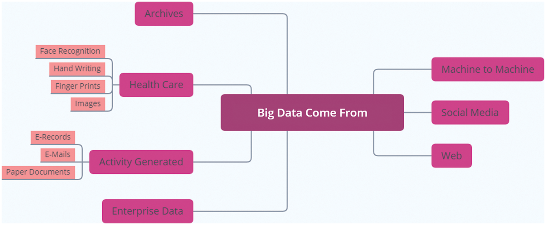
Figure 1: The variant sources of big data
The EHRs have many challenges we explain it as follows:
Quality: The underlying difficulty of receiving high-quality, reliable data in support of public health functions is not solved by just reporting laboratory data online rather than on paper. According to several researches, EHR does not increase data completeness. These findings show that there are still significant problems for the public health monitoring and informatics community to overcome beyond EHR implementation [6]. Improving poor data quality is one of these issues. Poor data quality is a widespread problem that affects all businesses and organizations that rely on information technology. Inaccurate data, inconsistencies between data sources, and inadequate or missing data necessary for operations or decisions are all common data quality challenges. The completeness of data in EHR systems has been shown to range from 30.7 percent to 100.0 percent in health care [7].
Costs and Time: Both the practices and the providers are burdened by the implementation of EHRs. EHRs are costly for practitioners, particularly individual practices that do not have the same resources as bigger health systems. Practices must not only purchase EHR software, but they must also hire professional IT personnel to provide support and training [8]. Training and the learning curve associated with EHR adoption consume a significant amount of time from physicians and personnel, time that could be spent on patient care. Errors are more likely to occur when employees are having difficulty adapting to or comprehending the system [9].
Accessibility: Because EHRs are kept electronically, they can be accessed at any time by different providers from various places. Providers can see a patient’s whole medical history, track treatment plans, and plan the course of care more efficiently. The accessibility of EHRs in a life-threatening situation can be lifesaving. Treatment decisions can be determined swiftly by reviewing a patient’s complete medical history, including allergies, blood type, and previous medical issues [10].
There are many methods for analyzing medical big data. These compile massive volumes of health and medical data in order to compare treatment efficiency, identify medicine and device safety issues, speed up medical research, and study shifting trends of patient features and diseases. Machine learning can be used to help automatic data inconsistency correction and data extraction from images, numeric, and textual data, such as reading text and extracting quality metrics or problems that were not previously on a patient’s problem list [11].
Our proposed method achieves a better result in comparison with other algorithms, which has two benefits, the reduction of data by decreasing the number of features and enhancing the classification accuracy. The goals of this paper are:
• Prediction and classification of different diseases occurrence using the proposed method.
• Using feature selection algorithm in combination with MDRL proposed algorithm to increase the accuracy.
• Presenting an ensemble approach with higher accuracy.
The rest of this paper is as follows: Section 2 shows the related work, Section 3 discusses the used methodologies, Section 4 displays our proposed ensemble model, Section 5 discusses the results and evaluation of our model and Section 6 includes the conclusion of our work.
Disease prediction is an important issue so, many researchers did their best to enhance the classification or prediction of medical data, we review it as follows. Subasi et al. [12] proposed a model using the M-health dataset. The Results explained that the proposed model with RF and SVM classification algorithms has the highest accuracy and is highly effective. The RF algorithm is most efficient with a high amount of data. The RF algorithm results in a high accuracy value. The resulted accuracy is 86%.
Baitharua et al. [13] experimented with many decision detection algorithms on liver disease dataset to predict decisions. They concluded Naïve Bayes is the least classifier algorithm and the Multilayer perceptron is the largest classifier algorithm with a 71.59% accuracy value. The MLP is good with a low volume of data but with big data, it is not efficient. Hafeez et al. [14] used the COVID-19 dataset. The prediction is performed by a classifier. They implemented a new classifier based on DT for enhancing performance accuracy and time. The supervised machine learning techniques including TSODT were developed to diagnose the COVID-19 illness victimization using the clinical information of the patients. The results expose that the suggested classifier algorithm provides the highest performance for medical applications with a 98% accuracy value.
Musa [15] applied the LR algorithm for different datasets. The LR classification algorithm is used to deal with the data with a single data point and expand to deal with data whose parameters are numbers and uncertain. The accuracy measurements vary from 76.3 to 95.2 by percent.
Botalb et al. [16] applied the MLP algorithm. The model was implemented on the EMNIST dataset which was used as 50% and 100% of its size. The models were trained with a fixed and flexible number of epochs in two runs. Using 100% of the dataset; for the fixed run, MLP achieved test accuracy of 31.43%, whereas the flexible run the MLP with 89.47% accuracy. Using 50% of the dataset; the accuracy for the MLP was 33.75%, wherein the flexible run of MLP was 88.20%.
Ramadhan et al. [17] applied a comparative analysis of accuracy for different algorithms using the K-Nearest Neighbor (KNN) and DT algorithms for the detection of the DDoS attacks dataset. The results explained that the accuracy of DT was higher than the KNN value, the accuracy of DT was 99.91%, and KNN has 98.94% of accuracy. KNN is not efficient with big data, the DT is more efficient.
Sathiyanarayanan et al. [18] used the DT algorithm under the supervised learning mechanism to detect breast cancer. Breast cancer recognition is conducted, which splits the data for the preparation and testing process. The result is compared between the algorithms KNN and DT. The results showed that the accuracy of KNN is 97%, while DT reaches the maximum accuracy of 99%. Therefore, a DT algorithm can predict the type of cancer efficiently.
Also, Osi et al. [19] examined and evaluated the execution of three various supervised machine learning techniques which are Linear Discriminant Analysis (LDA), RF, and Support Vector Machine (SVM) on the COVID-19 dataset. The best accuracy between these three algorithms was compared by some metrics for predictive performance such as accuracy, sensitivity, specificity, and F-score. The results showed that RF was the best algorithm with a 100% accuracy value in comparison with LDA and SVM with 95.2% and 90.9% respectively.
Benjamin et al. [20] executed three extremely general data mining techniques which are RF, NB, and DT to make a prediction system to predict the opportunity of heart diseases. Their basic aim was to detect the best classification algorithm which provides maximum accuracy. The UCI dataset of VA Long beach includes 270 instances and 13 heart disease attributes were used for training and testing processes. The dataset was split into 80% and 20% for training and testing respectively. Their results displayed that the RF classifier achieved better than NB and DT in the heart disease prediction. The RF is an efficient classification algorithm for medical big data.
Sridhar et al. [21] classified a heart disease model based on machine learning techniques depending on NB and DT algorithms in Python. The heart disease dataset was obtained from the Kaggle website, which includes 13 heart disease attributes. Another dataset used for simulation was collected from the UCI machine learning repository. The experimented model was done on the Scipy environment. Form their experimentations, the results displayed that the DT algorithm achieved better than the NB in the prediction of heart diseases.
Yahaya et al. [22] developed a heart disease prediction model to make an efficient diagnosis. They investigated many clinical systems for heart disease prediction. The classification algorithms such as the NB, DT, and Artificial Neural Network (ANN) have been implemented to detect heart diseases and evaluated to test the accuracies. Hence, only a minor achievement is done in the design of such predictive models for heart disease patients, therefore; there is a need for more complicated models that includes multiple different data sources to increase the accuracy of predicting the early occurrence of the disease. DT is the best predictive algorithm.
In our work, various classifier techniques are proposed that involve a combination of ensemble-based machine learning algorithms to detect the redundant features to enhance the accuracy and quality of heart disease, heart attack, covid-19, General health, and diabetes disease classification. We display an evaluation for the various diseases classification using five algorithms including our proposed model. The classifiers are evaluated by cross-validation with 4 folds method, and then we study the performance of MLP, DT, RF, LR, and our ensemble model (MDRL) classifiers. The basic role of this research is to find the best accuracy for the prediction of the different diseases by using major factors based on different classifier algorithms.
Tab. 1 shows a comparison between the related works of our work. It displays the tested data set, the implemented technique or techniques, the resulting accuracy value, and the comments on their works.
Classification is a data mining technique that classifies unstructured data into structured form. The classification has two main phases, the first is called the learning phase and the second phase is the prediction or test phase. The main role of classification in data mining is to predict the objective class from the training part of the dataset [23].
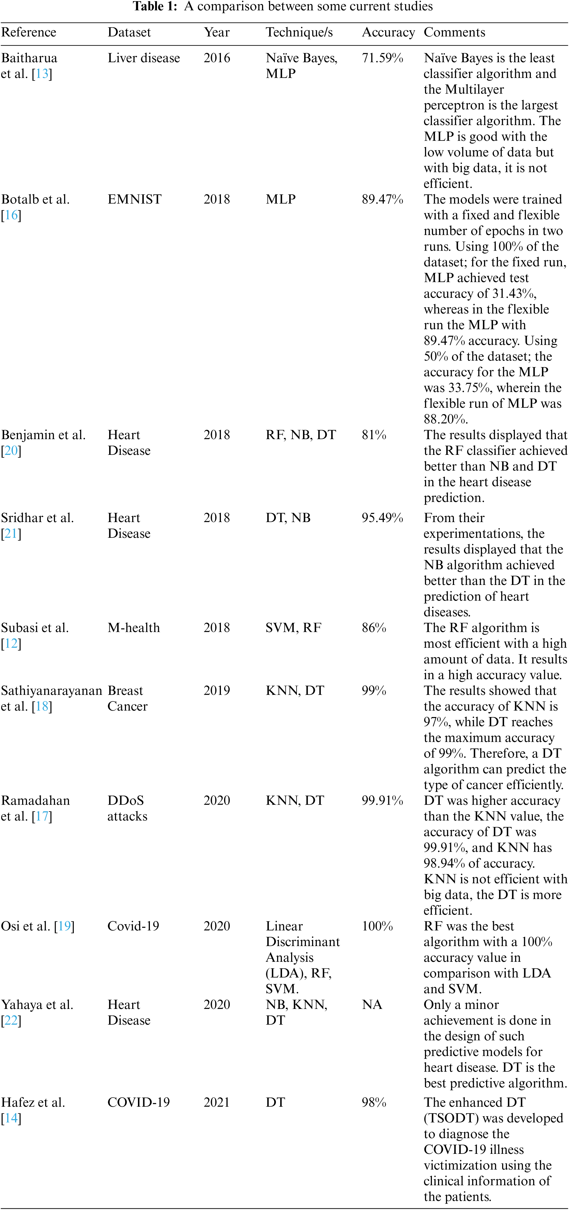
Neural Network (NN) simulated the human brain. It can learn the relationship of data. NN is based on a set of neurons. We implement the MLP classifier for NN. MLP is composed of at least three nodes layers input layer, hidden layer, and output layer. MLP used the backpropagation training technique [24]. The value of multipliers, often known as “weights,” across neurons of different layers is optimized during neural network training. The significance of these weights will be determined in order to eliminate errors in the output layer, of each interaction between the neurons [25].
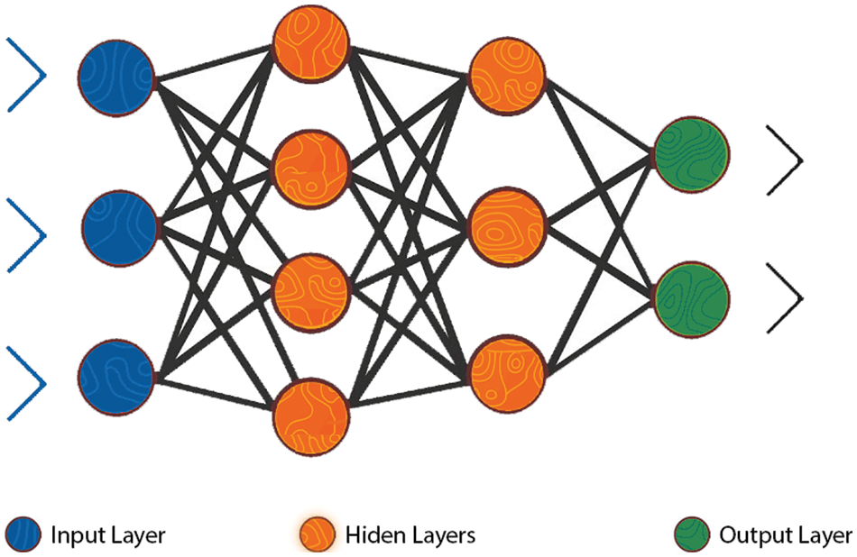
Figure 2: The MLP neural network structure [26]
We used some parameters to enhance the MLP accuracy as follows:
• hidden_layer_sizes (i,j) parameter which indicates the ith neuron’s number in the jth hidden layer.
• solver parameter which indicates the weight optimization may take one of the following values (lbfgs’, ‘sgd’, ‘adam’). We use ‘adam’ value; it is the best choice for a large dataset.
• random_state parameter indicates the random value for weights and bias initialization, and batch sampling when the solver is ‘sgd’ or ‘adam’.
Data is divided into hierarchical groups by DT. It’s a decision-making aid algorithm. Each internal node is a test property, the endpoint is a response or the class label, and each branch represents the classification rule, similar to a flowchart [27]. The following parameters are used to increase the decision tree’s performance:
• The max depth variable represents the tree’s maximum depth. Without this variable, the tree can be trapped in an infinite loop until all of the leaves have been expanded.
• A criterion parameter that represents the quality of such split. Entropy is a metric used to determine the amount of information gained.
Mutual information is a measure of information gain that is used for segmentation. This indicates how much information about a variable’s value you have. It’s the polar opposite of entropy, with a greater value indicating better performance. The data gain (S, 𝐴) is defined as the following on the definition of entropy, as shown in Eq. 2.
where the range of attribute 𝐴 is (𝐴), and 𝑆ν is a subset of set 𝑆 equal to the attribute value of attribute ν.
RF is an ensemble classification method that is ready to use. It’s a collection of trees, each of which is based on random factors [28]. The input value and a random variable are represented by the vector X = (X1, X2,…, Xn) T. The used joint distribution is PXY, and Y represents the response or forecast values (X, Y). Predicting Y from a prediction function f(X) is the goal [29]. The majority vote is used to forecast the class, which is defined as the most common class prediction between trees, so the voting takes place at the class probability level. The class with the highest class probability is chosen by the forecasts as shown in Fig. 3.
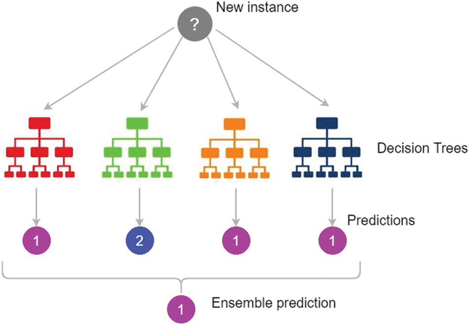
Figure 3: Random Forest prediction [30]
To improve our accuracy, we use the following RF parameters:
• The number of trees we need to generate before voting was represented by the n estimator’s option. The higher the number of trees, the better the accuracy, but it comes at the expense of performance time. For efficient classification, we use 50-100 tree numbers.
• The maximum depth of the trees is represented by the max depth option. It’s possible that if we don’t set a value for max depth, we’ll end up with endless nodes.
The random state parameter, allows easy replication of performance accuracy. Using random sample selections, the sub-trees can be repeated multiple times. These replications are controlled by random state’s initial value.
In the medical field, LR is a statistical technique. Each predictor was given a coefficient via LR. If the label is yes, the Y variable takes the (1) value, and if the label is no, the Y variable takes the (0) value. Binary logistic regression is used when the label has two values. When there are more than two values, however, the multinomial logistic regression is applied. [31].
The following parameters and attributes are used for accuracy enhancement:
• max_iter parameter which represents the maximum number of iterations until converge.
• random_state parameter which represents the random values used in shuffling.
• Classes attribute which represents the list of class labels to be obvious to the classifier.
Medical data are extremely complex and using one algorithm for classification to reach good results is difficult. For this reason, we use a combination of learning techniques to reach an efficient and accurate learning technique [32]. An ensemble is an asset of various algorithms which are running in parallel or sequentially, we run our algorithms parallel. The ensemble begins with inputting the training data to the base algorithm then voting is used to decide the best classifier in the ensemble. The voting classifier sums all the predictions of class labels, then the class label with the major value is chosen as the predicted class label. The voting classifier leads to better performance than any other model for the ensemble.
Our main challenge is to predict new medical data with high accuracy value and save processing time which is important to medical systems as it requires an accurate result. Medical data classification is a process that requires the following main steps: (i) data acquisition (ii) data preprocessing, (iii) feature extraction, and (iv) ensemble classified model as shown in Fig. 4. In the following sub-sections, we discuss these steps.
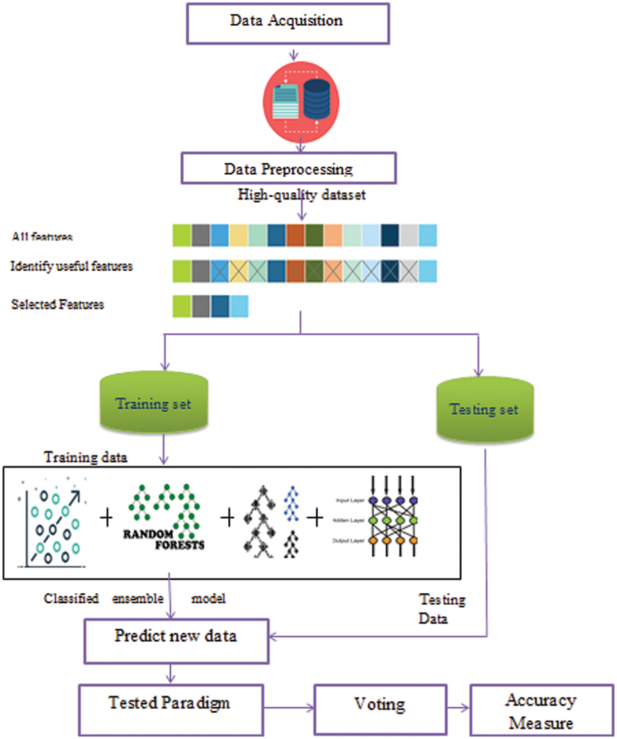
Figure 4: The Ensemble classification model for medical big data
The datasets are collected from different data resources. We collect data from different five sources. We use the following datasets heart disease dataset [33], Diabetes dataset [34], Health Care General Data [35], Covid-19 dataset [36], and Heart attack dataset [37]. These raw data have many problems. In the following phases, we explain and solve these problems.
The raw data is collected with different issues as missing values, noisy data, and redundant data that lead to bad accuracy results. Thus, it is necessary to remove noisy and redundant data and replace the missing values with the mean of its feature for numeric data and the “unknown” value for textual data. In addition, we use encoding as a preprocessing step. We use the One-Hot encoding mechanism. In One-Hot encoding, categorical variables are converted to numbers to be understood by the model. So, we use encoding to unit all the data forms to be able to run on different algorithms without any difficulties or problems. After this phase, the data used in training is more precise and accurate.
The data is collected with a wide variety of features that may not be useful and result in poor mining accuracy. Thus, it is important to use suitable features in the training step. Feature selection is an important step for data reduction. It removes irrelevant or redundant features. This step can improve classification accuracy. We use the most famous reduction algorithm which is the principal component analysis algorithm (PCA) and the correlation feature selection algorithm (CFS). For the PCA reduction algorithm, the basic variables are converted and projected onto a group of independent variables increasing the total variance in the system: the principal components [38]. The PCA is calculated as follows:
Calculate the mean of each feature by the equation:
Calculate the scatter matrix(S) by:
where m is the mean value
Calculate the covariance matrix with the eigenvector
where Σ is the Covariance matrix, v is the Eigenvector, and λ is the Eigenvalue
The CFS enhances classification accuracy and effectiveness. The CFS runs as follows: assume X is the set of all the features of the dataset with a large number of features {f1, f2, f3,….., fn} where n is the number of dataset’s attributes or features. The process of feature selection is selecting fi which generates x set of features with a smaller number of features [39]. As for a set of variables (X, Y), the linear correlation coefficient ‘r’ is calculated by:
4.4 Ensemble Data Classification
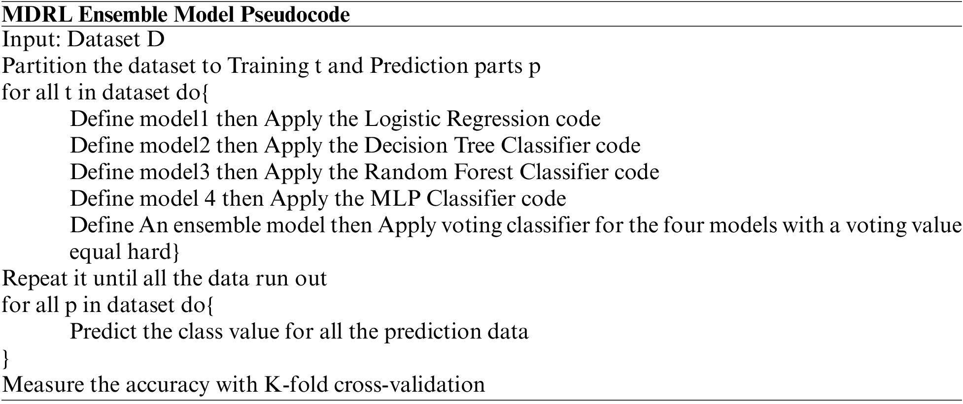
The data is divided into two sets the training data and the testing data. We divide it into 70% and 30%. We implement an ensemble model which is a set of four classification algorithms run parallel. These algorithms are LR, DT, RF, and MLP. We use the voting approach for deciding the best accuracy from all the classification algorithms. The voting value is hard. Finally, we use k-fold cross-validation for accuracy evaluation. The k-fold split’s number is four splits.
The experiments are done parallel on Windows 10, 64-bit operating system; processor Intel(R) 16 GB of RAM Core(TM) i7-7500 U CPU@ 2.70GHZ 2.90 GHz. We test the different techniques on five different datasets. We use Radoop, Weka, and Python 3.7 for implementation.
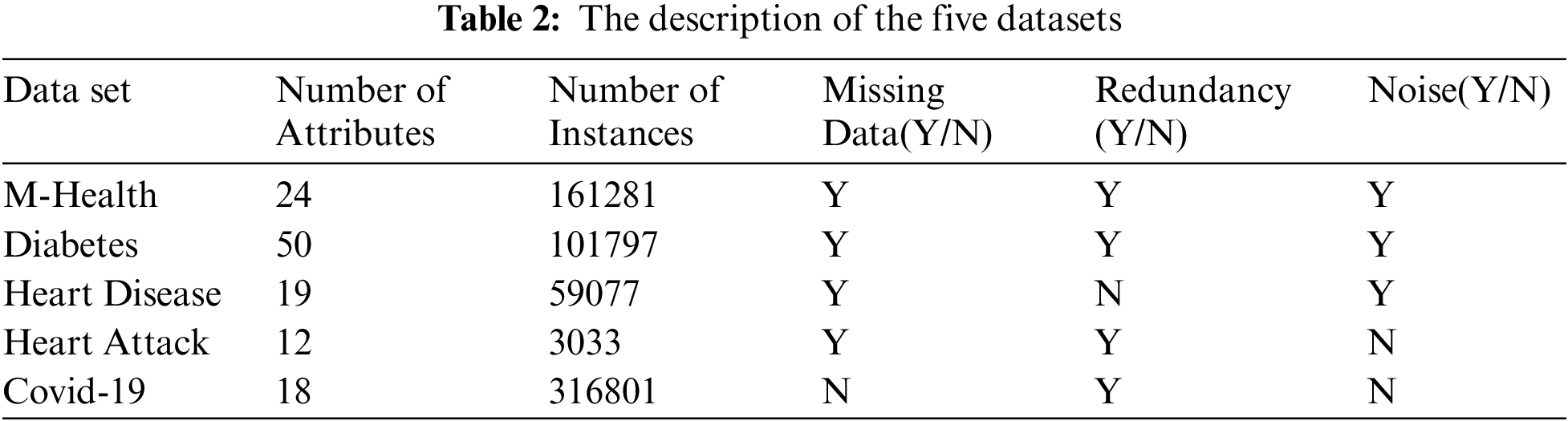
Tab. 2 shows the details of each dataset. The description of each dataset from the number of attributes, the instances numbers, is there a missing data or not, is there a missing data or not, is there a redundancy and noise or not. It shows if we use the encoding or feature selection on data or not.
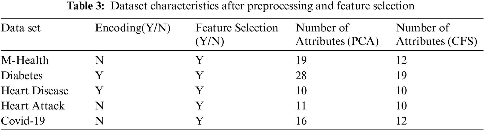
Tab. 3 shows the characteristics of the five datasets after preprocessing and feature selection steps. It displays which dataset is encoded and which one does not need encoding. Also, it displays whether the dataset needs feature selection or not. Adding, it explains the number of attributes after applying the CFS feature selection algorithm.
Tab. 4 shows the performance comparison of the different algorithms on the five datasets. Before implementing the classification, we apply a preprocessing and PCA feature selection algorithm on all datasets. We compare the accuracy, precision, recall, f-score, and time for the four classification algorithms and our proposed ensemble algorithm.
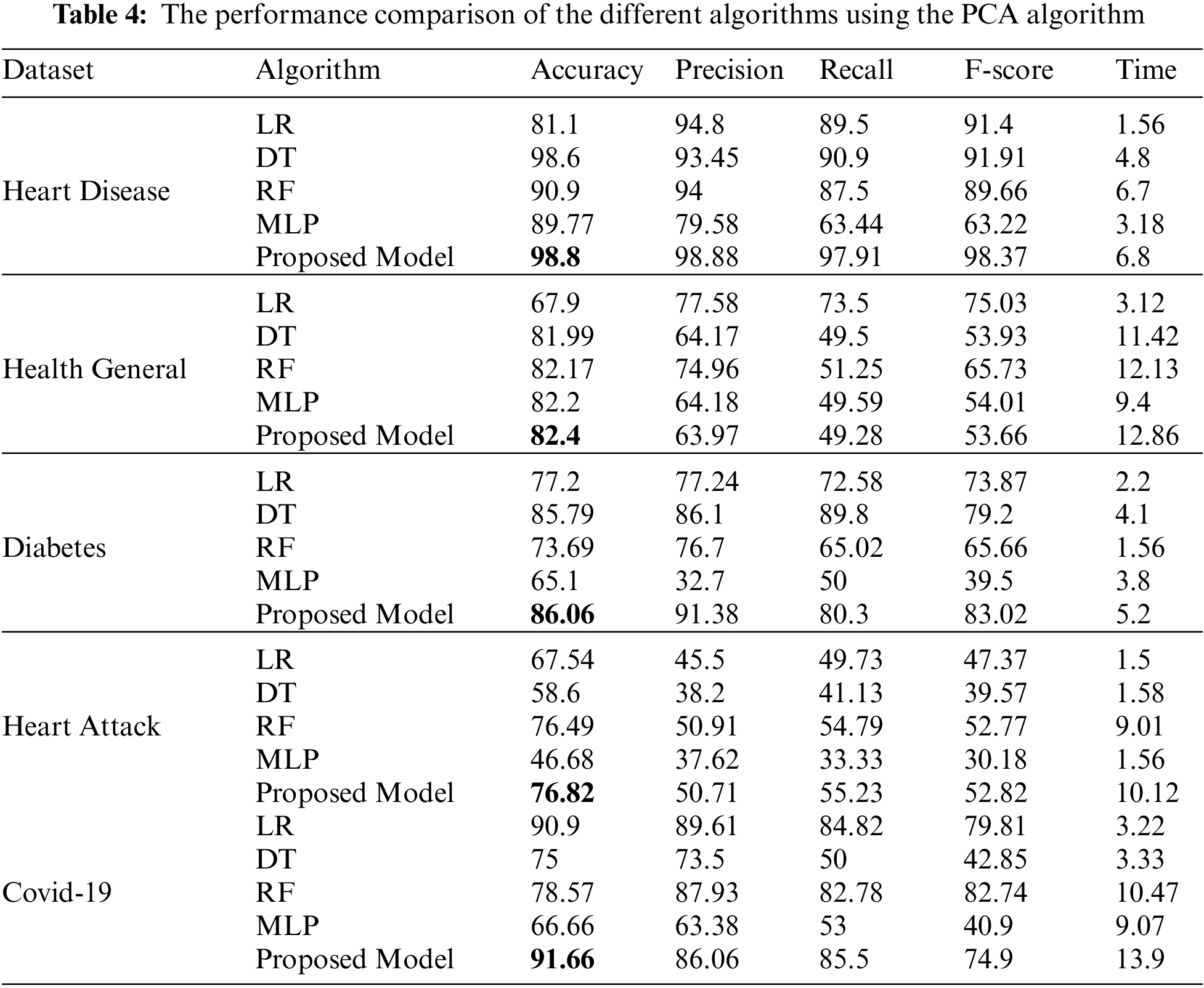
Tab. 4 shows the performance comparison for the different algorithms and our proposed model based on the PCA reduction algorithm on Heart Disease, Health General, Diabetes, Heart Attack, and Covid-19 datasets. The proposed model gives high accuracy values for all datasets. But, in comparison with Tab. 5 results, the CFS with our proposed model gave high-performance values than PCA with the model. Tab. 5 displays a comparison between the performances of the different algorithms when applied to the five datasets. The CFS feature selection algorithm is implemented on all datasets before applying the classification algorithms. The table’s comparison shows the accuracy, precision, recall, f-score, and time for each algorithm.
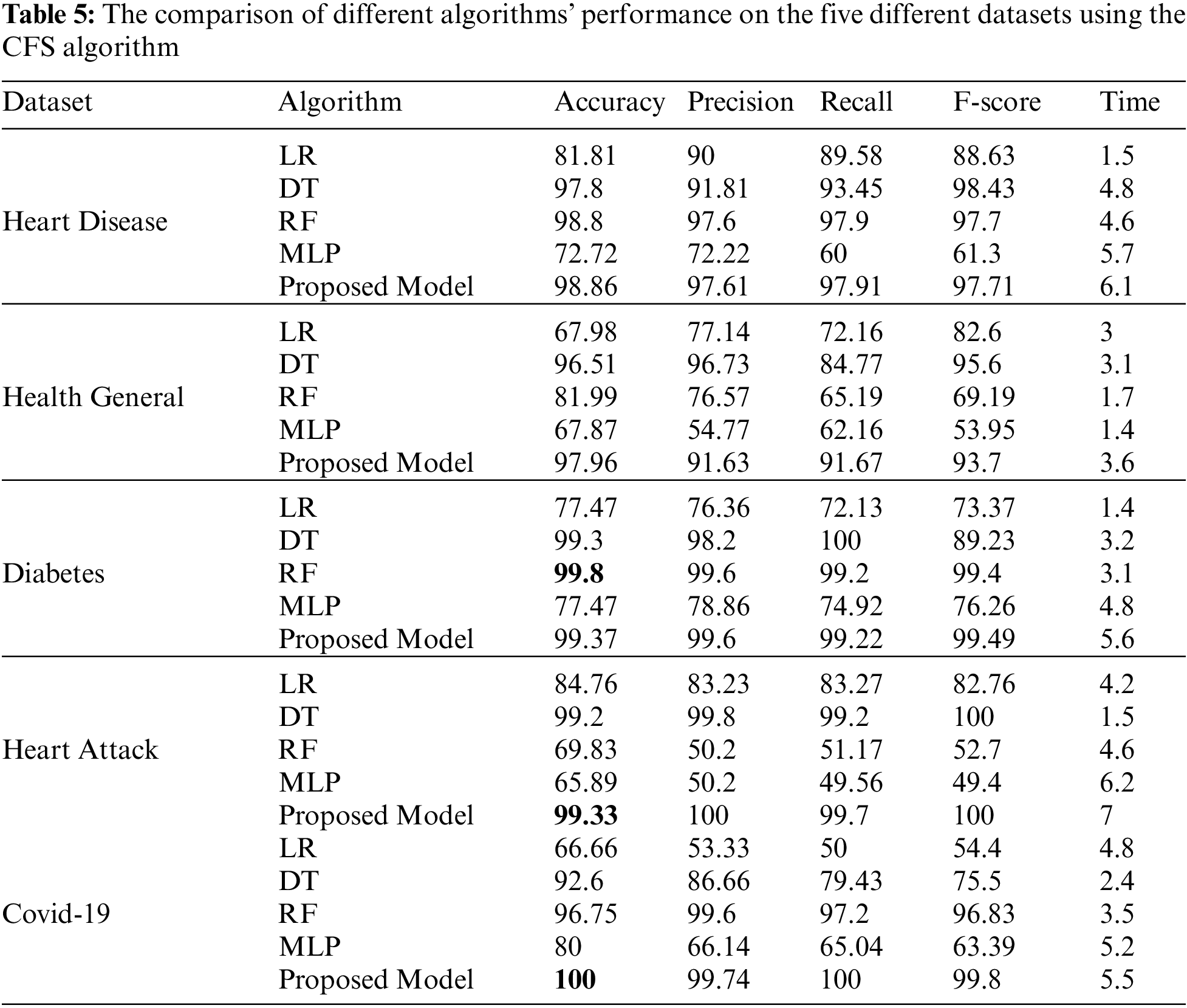
Python is the most accurate and efficient machine learning tool for big data classification. The classification is done in two steps: the training and predicting steps. Our experiments with big data classification by different five algorithms on five different datasets result in many consequences. Tabs. 4 and 5, and figures from 5 to 14 show that our ensemble model is efficient with variant datasets. The accuracy of our ensemble model is the best with Heart Disease, Health General, Heart Attack, and Covid-19 datasets. For the heart disease dataset, the accuracy of our ensemble model is 98.86%. The accuracy of our ensemble model for the Health General Dataset is 97.96%. For the Diabetes dataset, the highest accuracy is the RF algorithm with a 99.8% accuracy value. For the Heart Attack dataset, our ensemble model has the highest accuracy value with 99.33%. For the Covid-19 dataset, the best algorithm is our ensemble model with a 100 % accuracy value.
These formulas are used to compute the performance results:
The TP refers to the true positive value, TN is the true negative value, FP is the false positive value, and FN is the false negative value. To insure our approach efficiency, the accuracy is measured by using Eq. (7). The septicity is used to validate our model ability to detect negative patterns by using Eq. (8). The recall is measured to validate a classifier’s ability to detect positive patterns by Eq. (9). The F-score test’s accuracy, it is measured by Eq. (10).
Fig. 5 represents the comparison of accuracy, precision, recall, f-score, and time respectively for the heart disease dataset.
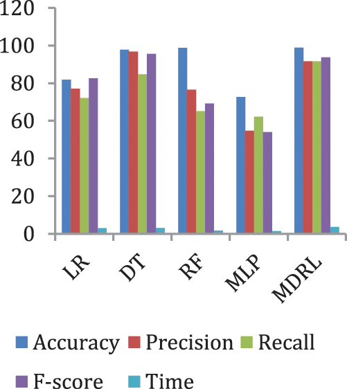
Figure 5: The accuracy, precision, recall, F-score, and time comparison of different algorithms for Heart Disease dataset
Fig. 6 represents the accuracy comparison between different algorithms applied on heart disease dataset based on PCA reduction algorithm and another test based on CFS reduction algorithm. Figs. 5 and 6 show that the accuracy of MDRL is the best with both PCA and CFS. The accuracy of MDRL with a combination of PCA is 98.8 and the accuracy of MDRL with a combination of CFS is 98.86. However, there is a little difference between both accuracy results but the combination with CFS is the best. The MDRL model with a combination of CFS gives the high performance results with 98.86 accuracy value, the precision value is 97.61, the value of recall is 97.91, and f-sore value is 97.71. The time consumption of the ensemble model for heart disease dataset is less than the time consumption of the four classification algorithms due to the parallel implementation. Hence, the time consumption of the ensemble model is 6.1s but the time of the four algorithms implementation is 16.6 s.
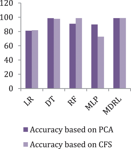
Figure 6: The accuracy comparison of different algorithms for Heart Disease dataset based on PCA and CFS algorithms
Fig. 7 represents the comparison of accuracy, precision, recall, f-score, and time respectively for the health general (M-Health) dataset. Fig. 8 represents the accuracy comparison between different algorithms applied on health general (M-health) dataset based on PCA reduction algorithm and another test based on CFS reduction algorithm. For a general dataset, when the size of the data increases, the accuracy of MDRL with a combination of PCA decreases. The accuracy of our model with PCA is 82.4 and for the model with CFS is 97.96. The performance time of the ensemble model for the Health General Dataset is 3.6 s but the time of the four algorithms implementation is 9 s. The MDRL model with a combination of CFS gives the high performance results with 97.96 accuracy value, the precision value is 91.63, the value of recall is 91.67, and f-sore value is 93.7.
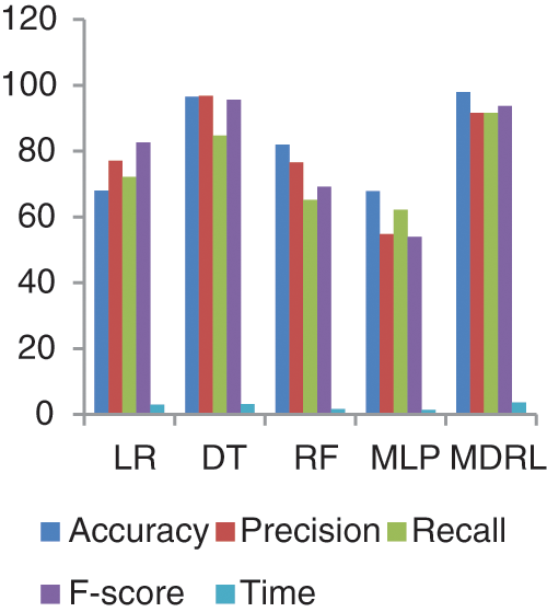
Figure 7: The accuracy, precision, recall, f-score, and Time comparison of different algorithms for Health general dataset
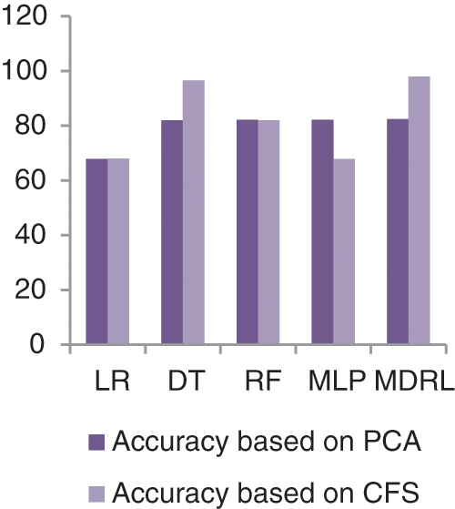
Figure 8: The accuracy comparison of different algorithms for Health general dataset based on PCA and CFS algorithms
Fig. 9 represents the comparison of accuracy, precision, recall, f-score, and time respectively for the Diabetes dataset. Fig. 10 represents the accuracy comparison between different algorithms applied on Diabetes dataset based on PCA reduction algorithm and another test based on CFS reduction algorithm. The time consumption of the ensemble model is 5.6 s but the time of the four algorithms implementation is 12.5 s. The ensemble model saves time consumption.
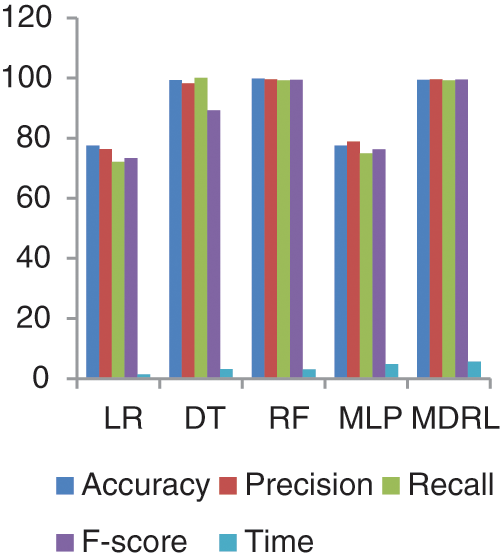
Figure 9: The accuracy, precision, recall, F-score, and time comparison of different algorithms for Diabetes dataset
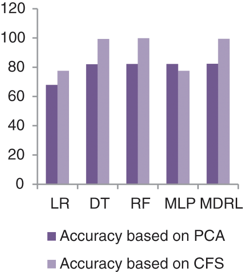
Figure 10: The accuracy comparison of different algorithms for Diabetes dataset based on PCA and CFS algorithms
From Fig. 9, we conclude that all algorithms with combination of CFS give high accuracy values than the combination with PCA. For our model the MDRL with PCA gives accuracy with 82.4 and for this combination with CFS the accuracy is 99.6. For the diabetes dataset, the MDRL model with a combination of CFS gives the high performance results with 99.37 accuracy value, the precision value is 99.6, the value of recall is 99.22, and f-score value is 99.49. But, the DT algorithm gives higher performance values with 99.8 accuracy value, the precision value is 99.6, the value of recall is 99.2, and the f-score value is 99.4.
Fig. 11 represents the comparison of accuracy, precision, recall, f-score, and time respectively for the Heart Attack dataset. Fig. 12 represents the accuracy comparison between different algorithms applied on Heart Attack dataset based on PCA reduction algorithm and another test based on CFS reduction algorithm. The time consumption of the ensemble model for Heart Attack Dataset is 7 s but the time of the four algorithms implementation is 16.5 s. From Figs. 11 and 12, it is shown that the MDRL with PCA and with CFS have the best accuracy than for other algorithms. The MDRL with CFS outperform the MDRL with PCA. The MDRL with CFS has best performance values with 99.33 accuracy value, 100 precision value, 99.7 for recall value, and 100 for f-score.
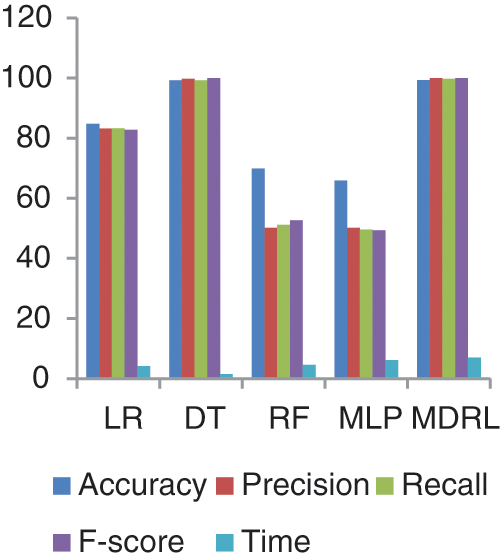
Figure 11: The accuracy, precision, recall, f-score, and time comparison of different algorithms for Heart Attack dataset
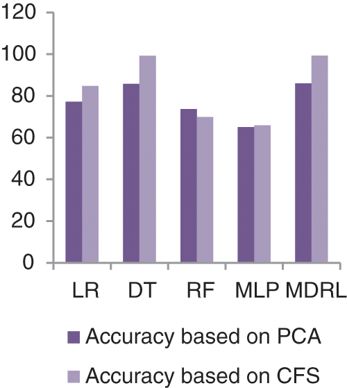
Figure 12: The accuracy comparison of different algorithms for Heart Attack dataset based on PCA and CFS algorithms
Fig. 13 represents the comparison of accuracy, precision, recall, f-score, and time respectively for the Covid-19 dataset.
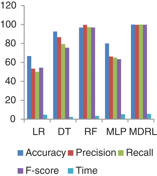
Figure 13: The accuracy, precision, recall, f-score, and time comparison of different algorithms for Covid-19 dataset
Fig. 14 represents the accuracy comparison between different algorithms applied Covid-19 dataset based on PCA reduction algorithm and another test based on CFS reduction algorithm. The accuracy of MDRL with PCA is 91.66 and with CFS is 100. Thus the accuracy of MDRL with CFS is the best. The time consumption of the ensemble model Covid-19 Dataset is 5.5 s but the time of the four algorithms implementation is 15.9 s. The ensemble model implementation saves time. From Fig. 13, the MDRL with CFS gives best performance values with 100 accuracy value, 99.74 precision value, recall value is 100, and 99.8 for f-score.
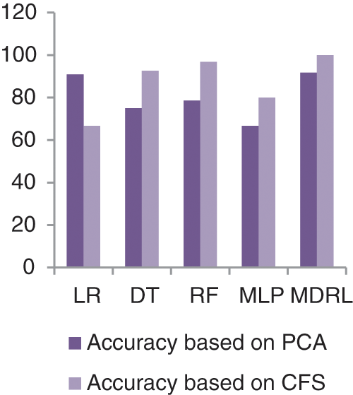
Figure 14: The accuracy comparison of different algorithms for Covid-19 dataset based on PCA and CFS algorithms
Tab. 6 compares the accuracy value of the M-health, Heart disease, Diabetes dataset when it is tested by the related work’s algorithm, our model based on PCA as feature selection algorithm, and our model based on CFS as feature selection algorithm.
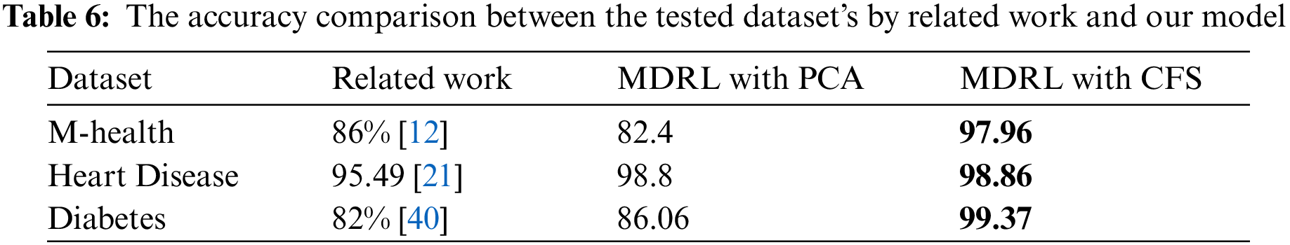
For the M-health, Heart disease, and Diabetes datasets, Tab. 6 shows a comparison between our proposed model MDRL based on PCA and CFS algorithms and the previous works. As indicated in the Tab. 6, our proposed model MDRL outperforms the other works for all datasets. This is done as we used a feature selection stage before classification step. We apply two different feature selection algorithms, the first one is the PCA and the second is CFS. From our table which compares the results, we conclude that the CFS algorithm is better in reduction of the data. From Tab. 6, the first three datasets explain that the MDRL based on CFS have the highest accuracy value than our model based on PCA and the previous works. The other two datasets, Covid-19 and Heart attack, are used to validate that our proposed model MDRL exceeds the current classification algorithms.
Experiments reveal that the suggested model produces results that are equivalent to those of alternative categorization techniques. We compare the results of four existing classification algorithms and our proposed ensemble model. The comparison done for five different datasets to insure the efficiency of our approach than others. The results show that our approach provides a high accuracy results than the traditional data classifications algorithms. Adding, we compare the results of our model with PCA and another time based on CFS. Then we compare these results with the accuracy of previous related works to insure the efficiency of our approach. The combination of MDRL with CFS gives the best performance values for variant datasets. We conclude that the CFS is a good reduction algorithm with high volume of data.
The potential issues of our approach
– The preprocessing aids in improving the accuracy as the good quality of data result in good performances.
– The applying of CFS data reduction algorithm decreases the processing time of the classification.
– The implementation of ensemble model increases the accuracy of most datasets.
The limitations of our approach
– Time complexity. However the ensemble model gives a high accuracy values, but it takes long time for execution.
– CPU processing complexity as the data has high volume size.
– Setting the parameters’ value take high effort and time as it is a try and error assignments.
The goal of this work was to introduce a methodology that had high recognition accuracy while avoiding the normal computational restrictions found in most existing research.
Ensemble learning is the implementation of multiple models, such as classifiers which are combined to solve a specific problem. Ensemble learning is used to enhance classification and prediction. Encoding is a very important step as we can use different data with different structures together without any difficulties. The feature selection is used for data reduction which improves the accuracy of the used dataset. The CFS reduction algorithm has the highest performance accuracy values with our ensemble algorithm in comparison to PCA with the same algorithm. Medical big data has special characteristics so; many traditional or well-known classification algorithms are not sufficient or accurate with it. From our experiments, we conclude that the ensemble model is efficient and gave a high accuracy value for variant datasets. Our ensemble model has high accuracy values of 98.86%, 97.96%, 100%, 99.33%, and 99.37% for heart disease, health general, covid-19, heart attack, and diabetes datasets respectively. For a comparison between our model with the previous works, we find that our model outperform the accuracy for all datasets. In the future, we intend to enhance our ensemble model to save the time processing as the ensemble model takes long time than the traditional algorithms. We aim to apply a feature selection algorithm with an ensemble model to enhance the processing time. Also, we suggest making a hybrid technique from our ensemble with another algorithm to increase the accuracy. Adding, we intend to make integration between the different types of data including medical images.
Funding Statement: The authors received no specific funding for this study.
Conflicts of Interest: The authors declare that they have no conflicts of interest to report regarding the present study.
1. N. A. AL Ajmi and M. S. Aksoy, “A review of big data analytic in healthcare,” Turkish Journal of Computer and Mathematics Education, vol. 12, no. 11, pp. 4542–4548, 2021. [Google Scholar]
2. G. Harerimana, B. Jang, J. W. Kim and H. K. Park, “Health big data analytics: A technology survey,” IEEE Access, vol. 6, pp. 65661–65678, 2018. [Google Scholar]
3. S. A. Lashari, R. Ibrahim, N. Senan and N. Sh. A. M. Taujuddin, “Application of data mining techniques for medical data classification: A review,” in MATEC Web of Conf., Malaysia, pp. 1–6, 2018. [Google Scholar]
4. G. Manogaran, P. M. Shakeel, S. Baskar, Ch. Hsu, S. N. Kadry et al., “FDM: Fuzzy-optimized data management technique for improving big data analytics,” IEEE Transactions on Fuzzy Systems, vol. 29, no. 1, pp. 177–185, 2021. [Google Scholar]
5. L. Hong, M. Luo, R. Wang, P. Lu, W. Lu et al., “Big data in health care: Applications and challenges,” Data and Information Management, vol. 2, no. 3, pp. 1–23, 2019. [Google Scholar]
6. P. Gatiti, E. Ndirangu, J. Mwangi, A. Mwanzu and T. Ramadhani, “Enhancing healthcare quality in hospitals through electronic health records: A systematic review,” Journal of Health Informatics in Developing Countries, vol. 15, no. 2, pp. 1–25, 2021. [Google Scholar]
7. C. N. Ta and C. Weng, “Detecting systemic data quality issues in electronic health records, in health and wellbeing e-networks for all, studies in health technology and informatics,” IOS press, vol. 264, pp. 383–387, 2019. [Google Scholar]
8. Common wealth fund, [Accessed on 7 January 2022]. Available: https://www.commonwealthfund.org/publications/newsletter-article/cost-biggest-barrier-electronic-medical-records-implementationqualitymaypotentiallymakethehealthcaresettingmoredangerous. [Google Scholar]
9. Se healthcare quality consulting, [Accessed on 7 January 2022]. Available: https://www.sehealthcarequalityconsulting.com/2018/09/18/the-benefits-andchallenges-of-electronic-health-records/. [Google Scholar]
10. M. Tayefi, Ph. Ngo, T. Chomutare, H. Dalianis, E. Salvi et al., “Challenges and opportunities beyond structured data in analysis of electronic health records,” Wires Computational Statistics, vol. 13, no. 6, pp. 1–19, 2021. [Google Scholar]
11. D. E. Adkins, “Machine learning and electronic health records: A paradigm shift,” American Journal of Psychiatry, vol. 174, no. 2, pp. 92–93, 2017. [Google Scholar]
12. A. Subasi, M. Radhwan, R. Kurdi and K. Khateeb, “IOT based mobile healthcare system for human activity recognition,” in 15th Learning and Technology Conf. (L&T), Jeddah, Saudi Arabia, pp. 29–34, 2018. [Google Scholar]
13. T. R. Baitharua and S. K. Panib, “Analysis of data mining techniques for healthcare decision support system using liver disorder dataset,” Procedia Computer Science, vol. 85, pp. 862–– 870, 2016. [Google Scholar]
14. M. A. Hafeez, M. Rashid, H. Tariq, Z. U. Abideen, S. S. Alotaibi et al., “Performance improvement of decision tree: A robust classifier using tabu search algorithm,” Applied Sciences, vol. 11, no. 15, pp. 1–17, 2021. [Google Scholar]
15. A. B. Musa, “Logistic regression classification for uncertain data,” Research Journal of Mathematical and Statistical Sciences, vol. 2, no. 2, pp. 1–6, 2014. [Google Scholar]
16. A. Botalb, M. Moinuddin, U. Al-Saggaf and S. S. Ali, “Contrasting convolutional neural network (CNN) with multi-layer perceptron (MLP) for big data analysis,” in Int. Conf. on Intelligent and Advanced System (ICIAS), Kuala Lumpur, Malaysia, pp. 1–5, 2018. [Google Scholar]
17. I. Ramadhan, P. Sukarno and M. A. Nugroho, “Comparative analysis of k-nearest neighbor and decision tree in detecting distributed denial of dervice,” in 8th Int. Conf. on Information and Communication Technology (ICoICT), Yogyakarta, Indonesia, pp. 1–4, 2020. [Google Scholar]
18. P. Sathiyanarayanan, S. Pavithra, M. S. Saranya and M. Makeswari, “Identification of breast cancer using the decision tree algorithm,” in IEEE Int. Conf. on System, Computation, Automation, and Networking (ICSCAN), Pondicherry, India, pp. 1–6, 2019. [Google Scholar]
19. A. A. Osi, M. Abdu, U. Muhammad, A. Ibrahim et al., “A classification approach for predicting COVID-19 patient survival outcome with machine learning techniques,” Science Forum Journal of Pure and Applied Sciences, vol 22, pp. 1–25, 2020. https://doi.org.10.5455/sf.aaosi2. [Google Scholar]
20. H. Benjamin, F. David and S. A. Belcy, “Heart disease prediction using data mining techniques,” ICTACT Journal of Soft Computing, vol. 9, no. 1, pp. 1824–1830, 2018. [Google Scholar]
21. A. Sridhar and A. Kapardhi, “Predicting heart disease using machine learning algorithm,” International Research Journal of Engineering and Technology, vol. 6, no. 4, pp. 36–38, 2018. [Google Scholar]
22. L. Yahaya, N. D. Oye and E. J. Garba, “A comprehensive review on heart disease prediction using data mining and machine learning techniques,” American Journal of Artificial Intelligence, vol. 4, no. 1, pp. 20–29, 2020. [Google Scholar]
23. R. Chen, C. Dewi, S. Huang and R. E. Caraka, “Selecting critical features for data classification based on machine learning methods,” Journal of Big Data, vol. 7, no. 52, pp. 1–26, 2020. [Google Scholar]
24. J. C. Chen and Y. M. Wang, “Comparing activation functions in modeling shoreline variation using multilayer perceptron neural network,” MDPI Water, vol. 12, no. 5, pp. 1–12, 2020. [Google Scholar]
25. N. F. S. Neto, S. F. Stefenon, L. H. Meyer, R. Bruns, A. Nied et al., “A study of multilayer perceptron networks applied to classification of ceramic insulators using ultrasound,” Applied Sciences, vol. 11, no. 2, pp. 1592, 2021. [Google Scholar]
26. Medium, [Accessed on 13 December 2021]. Available: https://medium.datadriveninvestor.com/artificial-neural-network-nn-explained-in-5-minutes-with-animations-9a80f49ab190. [Google Scholar]
27. L. J. Muhammad, M. M. Islam, S. S. Usman and S. I. Ayon, “Predictive data mining models for novel coronavirus (COVID 19) infected patients’ recovery,” SN Computer Science, vol. 1, no. 5, pp. 200–206, 2020. [Google Scholar]
28. S. Raj, S. Singh, A. Kumar, S. Sarkar and C. Pradhan, “Feature selection and random forest classification for breast cancer disease,” in: Data Analytics in Bioinformatics, First Edition ed., USA: John Wiley & Sons, Inc, pp. 191–210, 2021. [Google Scholar]
29. R. Genuer and J. M. Poggi, “Random forests,” in: Random Forest in R, First Edition ed., Cham: Springer, pp. 33–51, 2020. [Google Scholar]
30. Medium, [Accessed on 13 December 2021]. Available: https://medium.com/m/globalidentity?redirectUrl=https%3A%2F%2Ftowardsdatascience.com%2Frandom-forests-an-ensemble-of-decision-trees-37a003084c6c. [Google Scholar]
31. E. Y. Boateng and D. A. Abaye, “A review of the logistic regression model with emphasis on medical research,” Journal of Data Analysis and Information Processing, vol. 7, no. 4, pp. 190–207, 2019. [Google Scholar]
32. X. Dong, Z. Yu, W. Cao, Y. Shi and Q. Ma, “A survey on ensemble learning,” Frontiers of Computer Science, vol. 14, no. 5, pp. 241–258, 2019. [Google Scholar]
33. Catalog.datagov, [Accessed on 20 March 2021]. Available: https://catalog.data.gov/dataset/heart-disease-mortality-data-among-us-adults-35-by-state-territory-and-county. [Google Scholar]
34. Kaggle, [Accessed on 11October 2021]. Available: https://www.kaggle.com/brandao/diabetes?select=diabetic_data.csv. [Google Scholar]
35. O. Banos, R. Garcia, J. A. Holgado-Terriza, M. Damas, H. Pomares et al., “mHealthDroid: A novel framework for agile development of mobile health applications,” in 6th Int. Work-conf. on Ambient Assisted Living an Active Ageing, Cham, Springer, pp. 91–98, 2014. [Google Scholar]
36. Kaggle, [Accessed on 20 March 2021]. Available: https://www.kaggle.com/iamhungundji/covid19-symptoms-checker. [Google Scholar]
37. Kaggle, [Accessed on 20 March 2021]. Available: https://www.kaggle.com/nareshbhat/health-care-data-set-on-heart-attack-possibility. [Google Scholar]
38. M. Sidharth, S. Uttam, T. Subhash, D. Sanjoy, S. Devi et al., “Principal component analysis,” International Journal of Livestock Research, vol. 7, no. 5, pp. 60–78, 2017. [Google Scholar]
39. M. Doshi and K. C. setu, “Correlation based feature selection (CFS) technique to predict student performance,” International Journal of Computer Networks & Communications (IJCNC), vol. 6, no. 3, pp. 197–206, 2014. [Google Scholar]
40. Kaggle, [Accessed on 7 December 2021]. Available: https://www.kaggle.com/paultimothymooney/predict-diabetes-from-medical-records. [Google Scholar]
 | This work is licensed under a Creative Commons Attribution 4.0 International License, which permits unrestricted use, distribution, and reproduction in any medium, provided the original work is properly cited. |