DOI:10.32604/cmc.2022.027415
| Computers, Materials & Continua DOI:10.32604/cmc.2022.027415 | |
| Article |
CNN-BiLSTM-Attention Model in Forecasting Wave Height over South-East China Seas
1School of Artificial Intelligence (School of Future Technology), Nanjing University of Information Science and Technology Nanjing, 210044, China
2Southern Marine Science and Engineering Guangdong Laboratory (Zhuhai), Zhuhai, 519080, China
3School of Marine Sciences, Nanjing University of Information Science and Technology, Nanjing, 210044, China
4International Business Machines Corporation (IBM), New York, 10504, USA
*Corresponding Author: Lina Wang. Email: wangln@nuist.edu.cn
Received: 18 January 2022; Accepted: 19 April 2022
Abstract: Though numerical wave models have been applied widely to significant wave height prediction, they consume massive computing memory and their accuracy needs to be further improved. In this paper, a two-dimensional (2D) significant wave height (SWH) prediction model is established for the South and East China Seas. The proposed model is trained by Wave Watch III (WW3) reanalysis data based on a convolutional neural network, the bi-directional long short-term memory and the attention mechanism (CNN-BiLSTM-Attention). It adopts the convolutional neural network to extract spatial features of original wave height to reduce the redundant information input into the BiLSTM network. Meanwhile, the BiLSTM model is applied to fully extract the features of the associated information of time series data. Besides, the attention mechanism is used to assign probability weight to the output information of the BiLSTM layer units, and finally, a training model is constructed. Up to 24-h prediction experiments are conducted under normal and extreme conditions, respectively. Under the normal wave condition, for 3-, 6-, 12- and 24-h forecasting, the mean values of the correlation coefficients on the test set are 0.996, 0.991, 0.980, and 0.945, respectively. The corresponding mean values of the root mean square errors are measured at 0.063 m, 0.105 m, 0.172 m, and 0.281 m, respectively. Under the typhoon-forced extreme condition, the model based on CNN-BiLSTM-Attention is trained by typhoon-induced SWH extracted from the WW3 reanalysis data. For 3-, 6-, 12- and 24-h forecasting, the mean values of correlation coefficients on the test set are respectively 0.993, 0.983, 0.958, and 0.921, and the averaged root mean square errors are 0.159 m, 0.257 m, 0.437 m, and 0.555 m, respectively. The model performs better than that trained by all the WW3 reanalysis data. The result suggests that the proposed algorithm can be applied to the 2D wave forecast with higher accuracy and efficiency.
Keywords: Conv2D; CNN-BiLSTM-Attention; wave forecasting; significant wave height; typhoon
As a statistical variable, the ocean’s significant wave height is an extremely important indicator in marine engineering, maritime navigation, and transport [1,2]. It is also an important parameter for marine disaster prediction [3] and sustainable renewable energy [4]. Currently, the most widely used prediction models are the third-generation numerical wave prediction models (e.g., Wave Modeling, Wave Watch III, and Simulating Waves Nearshore). They are computational models based on energy balance equations that consider various physical processes [5]. However, these models have the disadvantages, such as complex calculation process, long running time, and high prediction cost, and cannot achieve fast and accurate prediction. The significant wave height is nonlinear and asymmetrical, which is affected by climatic conditions, seasonal characteristics, and topographical factors. Machine learning methods can fit complex nonlinear processes and solve complex nonlinear problems of the physical mechanism without prior knowledge of the system. Therefore, they are applied into significant wave height prediction, involving single prediction models and composite prediction models. The single prediction models include artificial neural network (ANN) [6], recurrent neural network (RNN) [7], support vector machine (SVM) [8], etc. The composite prediction models are comprised of wavelet transform neural network (WLNN) [9], hybrid empirical mode decomposition support vector regression model (EMD-SVR) [10], extreme learning machine model integrated with improved complete ensemble empirical mode decomposition (ICEEMDAN-ELM) [11], multiple linear regression based on the covariance-weighted least squares model (MLR-CWLS) [12], etc. These models perform well in short-term prediction, and the prediction results of the composite network have higher accuracy. The machine learning method can fit the nonlinear process well, but it relies on extracting data features, and the generalization ability needs to be improved. The deep learning method can automatically learn the inherent law and representation level of the samples, providing strong support for ocean prediction. The existing deep learning methods to predict the significant wave height include Long Short-Term Memory (LSTM) [13], Convolutional Neural Network-Long Short-Term Memory (CNN-LSTM) [14], etc. However, most of these models have simple structures and cannot fully mine the correlation among data. The multi-layer neural network can fully extract data features [15]. Zhou et al. constructed a multi-layer deep learning network ConvLSTM and applied it to wave prediction in the South and East China Seas, achieving good prediction results [16]. Mooneyham et al. [17] combined the convolutional neural network (CNN) with the SWRL network to develop a new method for near-shore wave prediction. Yang et al. [18] proposed a new method for wave prediction by combining STL decomposition, CNN and position coding, and verified the algorithm by using significant wave height data of three buoy stations.
CNN can be used for deep feature extraction from massive data. However, it is difficult to obtain the associated information between time-series data, which affects the prediction effect of the model. The bidirectional long short-term memory network (BiLSTM) model is applied to fully extract the features of the associated information of time series data and improve the prediction accuracy of the model considering the effect of two-way information flow [19]. To fully extract spatial features of significant wave height, avoid information loss, and improve prediction accuracy, this paper proposes a prediction method based on CNN-BiLSTM-Attention. Considering the nonlinearity and asymmetry of significant wave height, CNN is introduced to extract the spatial features of the original wave height data to reduce the redundant information input into the BiLSTM network. Meanwhile, the attention mechanism [20] is applied to assign a probability weight to the output information of BiLSTM layer units, and a training model is constructed. Compared with the ConvLSTM model [16], a similar layer structure of ConvLSTM and a Convolution layer are set in the CNN-BiLSTM-Attention model. CNN-BiLSTM-Attention can fully extract the spatial local features of the data and train the output features after processing. In this way, the prediction model is obtained, and it is applied to the coastal waters in the northwestern Pacific Ocean (105°E–126°E, 4°N–43°N). Finally, a two-dimensional significant wave height prediction model is established and its validity is verified by examples.
2.1.1 Significant Wave Height Reanalysis Product
In this study, the significant wave height (SWH) data from the reanalysis dataset of the third-generation numerical wave model (WW3) produced by the National Oceanic Atmospheric Administration (NOAA) are obtained to train and test the proposed model. The study area is selected from the South and East China Seas in the northwest Pacific coastal waters at 105°E–126°E and 4°N–43°N, as is shown in Fig. 1. The study period is from 2011 to 2020. The temporal resolution of the data is hours, and the spatial resolution is 0.5° × 0.5°.

Figure 1: The area of South and East China Seas in the northwest Pacific coastal waters at 105°E–126°E and 4°N–43°N
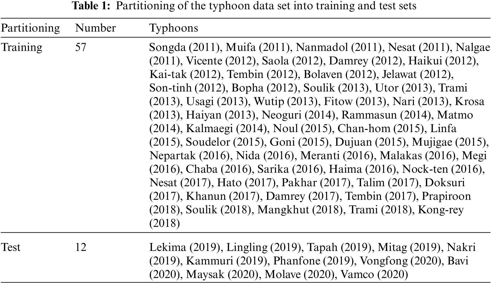
Typhoons in the coastal waters of the study area at 105°E–126°E and 4°N–43°N from 2011 to 2020 are selected to generate the typhoon-induced SWH data set (the maximum Beauford wind force is above 12, and the central wind speed ranges from 32.7 to 41.4 m/s). Typhoon data are acquired from the Typhoon Network of the Central Meteorological Observatory. The typhoon data set consists of 71 data sets of typhoon data, including 57 data sets from 2011 to 2018 as training sets, and 12 data sets from 2019 to 2020 as test sets. The specific information of the typhoon data is shown in Tab. 1. Here, the cases of SWH prediction when typhoons occur are given, and the prediction results of SWH when typhoons in the test set occur are analyzed.
2.2.1 Convolutional Neural Network
CNN [21] is a kind of deep Neural Network. CNN usually includes convolution layers, pooling layers, and a full-connected layer. The convolution layer uses a sliding window to perform convolution operations on the input data. The pooling layer samples the feature maps, and the pooling operation can reduce the amount of data and keep useful information. The full-connected layer performs regression processing on the features extracted from layer-by-layer transformation and mapping. The convolution operation is shown in Eq. (1):
where
where
where
2.2.2 Long Short-Term Memory Network
LSTM network was first proposed by Hochreiter et al. [22]. Based on the recurrent neural network (RNN), the gate structure is introduced, which can effectively solve the problems of gradient disappearance and overcomes the defects in the long-term dependence of RNN. The LSTM network structure includes forgetting gates, input gates, output gates and memory units. LSTM carries out the selective memory of the information in the cell state, reserves useful information and transmits it forward, forgets useless information, and outputs the hidden layer state at each moment. The structure of an LSTM neuron is shown in Fig. 2.

Figure 2: The structure of an LSTM neuron
The functions and gates within the LSTM neuron are calculated as follows:
where
Since the LSTM network has a certain limit in memory capacity and can only process one-way time-series information, the information at the later moment cannot play a role in the previous information. However, in the actual prediction task, the state at the current moment may be affected by the input and the state of the previous and subsequent moments. Therefore, BiLSTM is introduced in this paper. BiLSTM adds a layer of reverse LSTM based on the LSTM network to process reverse time series [23]. The bidirectional structure of BiLSTM can enhance the ability to deal with nonlinear time series, improve the dependence of the long-term time, and strengthen the performance of neural networks, thus obtaining more accurate prediction results. The structure of BiLSTM is shown in Fig. 3.

Figure 3: The BiLSTM network structure
In Fig. 3,
where the function
The attention mechanism simulates the human brain focusing on a particular area at a particular moment, selectively acquiring more useful information, and ignoring useless information [24,25]. It can strengthen the influence of key information and enhance the accuracy of model judgment by assigning different weight values to the hidden layer units of a neural network. Adopting the attention mechanism enables the model to learn reasonable vector representations and makes the key information dominate the prediction process, thereby improving the prediction accuracy of the model.
The data are processed by the attention mechanism according to Eqs. (12)–(14):
where
3 Wave Forecast Model Based on CNN-BiLSTM-Attention Algorithm
The specific structure of the prediction model based on CNN-BiLSTM-Attention is shown in Fig. 4. The SWH of three continuous time steps are taken as the input, and the extracted features through the three layers of Conv2D are taken as the input of the BiLSTM-Attention model. After two layers of BiLSTM, the Attention layer is added. Finally, the full-connected layer adjusts the feature dimension and outputs the SWH data at a certain time in the future. In this model, the ReLU function is employed as activation function in Conv2D and Dense layers, and

Figure 4: The structure of the CNN-BiLSTM-Attention model
Compared with the existing CNN-BiLSTM-Attention models [26–28], this paper implements Conv2D rather than Conv1D as the geological position information embedded in the significant wave height data. This information is very important for wave height prediction. Exerting convolution by flattening data with Conv1D will make the confusion of the data from different observational sites far away from each other on the map. To extract more features by convolution, the MaxPooling option needs to be discarded.
Firstly, the input data are preprocessed, and the local deep features of the data are extracted by Conv2D. Then, the extracted multiple feature vectors are transmitted to the BiLSTM-Attention network for training. The influence of past information and future information on the current information is considered, and the key information is assigned a higher weight. During the training process, the Dropout layer is used to randomly discard some characteristics to improve the robustness of the model, and the prediction model is obtained. Finally, the predicted values in the test set are output, and the error analysis is given. The flowchart of the model is shown in Fig. 5.

Figure 5: The flow of CNN-BiLSTM-Attention algorithm
In this section, the proposed algorithm is applied to wave height prediction in the South and East China Seas, and the model is verified and discussed under normal and extreme typhoon-forced cases, respectively. This section consists of two parts. The first part involves the forecast of SWH under normal wave conditions is analyzed and discussed. The second part involves the analysis and discussion of the prediction results of SWH under the extreme condition forced by a typhoon. At the stage of model training, the number of epochs is set to 10.
In this study, the WW3 significant wave height data from the reanalysis product released by NOAA from 2011 to 2020 are used as the experimental data set. The study area is at 105°E–126°E and 4°N–43°N. The spatial resolution is 0.5 × 0.5°. Considering the timeliness of waves, the input data used in this study are wave field data at three continuous moments. According to the difference of forecast time step (e.g., 1, 2, and 3 h), the first 70% of this data set is used as a training set and verification set, and the last 30% as a test set. In the SWH prediction under normal conditions, the SWH data from 12:00 on June 14, 2018, to 23:59 on December 31, 2020 is used as the test set. These data are not involved in the training of the model to ensure the independence of the training and test sets. In addition, the training and test sets for extreme cases (typhoons) are based on statistical typhoon events, and the SWH data when a typhoon occurred over the period 2011–2020 are selected. The data from 57 typhoon events are used as a training set, and the data from 12 typhoon events are used as a test set. To improve the model performance, the data of the training and test sets are normalized before model training.
The mean absolute error (MAE), root mean square error (RMSE), Pearson correlation coefficient (Correlation), as well as the mean values of the three evaluation indexes in the test sample space (M_MAE, M_RMSE, M_Correlation) are used to evaluate the error and deviation between the prediction value and the WW3 reanalysis data value and measure the linear correlation between the predicted value and the WW3 reanalysis data value. The specific expression is as follows:
where
4.3 Wave Forecast Under Normal Conditions
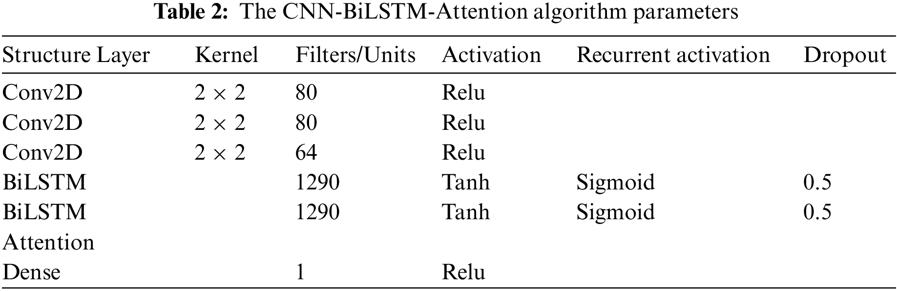
In this section, the CNN-BiLSTM-Attention algorithm is applied to SWH data prediction under normal wave conditions. The parameter selected by the algorithm is shown in Tab. 2.
To study the prediction results of the model, a case is selected to analyze the process. The prediction result of SWH under normal conditions is evaluated, and the results are shown in Fig. 6. The input data are SWH at 11:00, 12:00, and 13:00 on March 20, 2020.
Figs. 6a–6e shows the distribution of the predicted SWH after 1, 3, 6, 12, and 24 h. Figs. 6f–6j shows the distribution of the WW3 wave fields at the corresponding time. Figs. 6k–6o shows the spatial distribution of the absolute errors between the predicted value and the actual value at the corresponding moment. It can be seen from Fig. 6a that the 1-h prediction result is the best, which is almost consistent with the spatial distribution of the real SWH and has the highest correlation value. In the 1-h prediction, referring to Fig. 6k, the absolute prediction error is within 0.1 m in most areas, and between 0.1 m and 0.2 m in a few areas. It can be observed that when the prediction time is 1 h, the proposed model has the best prediction ability in the given ocean region, and accurate numerical values and spatial distribution patterns can be obtained both in the area with relatively high values in the open sea and gulf or the area with relatively low SWH. As the prediction time increase, the absolute error increases, and the correlation decreases. In Fig. 6l, the prediction error increases significantly in the East China Sea (ECS), while the relatively large prediction errors begin to appear in the Yellow Sea. In Fig. 6m, the error at this moment mainly comes from the prediction results of the Yellow Sea and the ECS. In addition, the absolute error in the Bohai Sea and the South China Sea (SCS) also increases. If the prediction interval is increased to 12 h, the prediction errors in all sea areas further increase, as shown in Fig. 6n. The error of predicting SWH in the ECS, the Bohai Sea, and the Yellow Sea is more significant, and the prediction error also increases in some areas of the SCS. Finally, the 24-h prediction result is the worst and has the largest absolute error.
In Fig. 7, when zero values of SWH are removed, the predicted values and true values of SWH at the corresponding time span in Fig. 6 are expanded line by line from low to high latitudes. The input data are the SWH at 11:00, 12:00, and 13:00 on March 20, 2020. In Fig. 7a, the predicted value at each grid point is almost consistent with the true value, and the Correlation, RMSE, and MAE are 0.997, 0.035 m, and 0.018 m, respectively. If the forecast time span is increased to 3 h, the model can still guarantee a high prediction accuracy. However, the correlation coefficient decreases to 0.995 with the increase of the forecast error in Fig. 7b. If the prediction interval is increased to 6 h, the correlation coefficient will decrease to 0.988. As is shown in Fig. 7c, the predicted value is generally greater than the true value with the increasing fluctuation of the prediction error. The deviation of the predicted value from the true value becomes larger with a correlation coefficient of 0.971, as shown in Fig. 7d. If the prediction interval is increased to 24 h, the predicted value is not consistent with the true value at most observation points in Fig. 7e, corresponding to the worst forecast performance of the model.

Figure 6: Wave height prediction results obtained by the CNN-BiLSTM-Attention algorithm at the (a) 1-, (b) 3-, (c) 6-, (d) 12- and (e) 24-h forecast time span. These forecasts are based on WW3SWHs at 11:00, 12:00, and 13:00 on March 20, 2020. Observations for each forecast time span are provided in (f)–(j). The absolute errors between these are given in (k)–(o)

Figure 7: Comparisons between forecast values (red) and observed values (blue) of all sample points at the (a) 1-, (b) 3-, (c) 6-, (d) 12-, and (e) 24-h forecast time span
Furthermore, to study the prediction performance of the model in the test sample space, three indexes are adopted, including the mean of correlation coefficient (M_Correlation), the mean of root mean square error (M_RMSE), and the average mean absolute error (M_MAE). The values of the three evaluation indexes have been calculated for the CNN-BiLSTM-Attention algorithm. The prediction results of wave height under normal conditions are presented in Tab. 3.
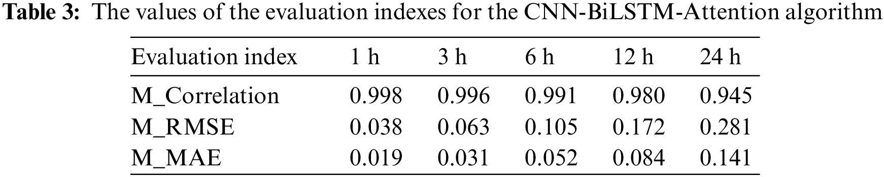
It can be seen from Tab. 3 that with the increase of the forecast time span, the M_Correlation between the predicted values and the true values in the test set becomes lower, and the forecast errors including M_RMSE and M_MAE become larger. The 24-h prediction result is the worst with the lowest M_Correlation and the largest M_RMSE and M_MAE.
4.4 Wave Forecast Under Extreme Conditions
Typhoons are typical low-pressure systems that are characterized by a significant convergence of air flow toward the center at the low layer, and the air flow at the top layer mainly exhibits outward divergence [29,30]. Usually, when a typhoon passes over the sea, the wind speed on the sea surface increases, and the wave height also increases. A strong typhoon may induce waves up to 10 m in height. In the ECS, typhoons mainly occur from July to September. In the SCS, typhoons occur frequently in May/June and October to December [31]. Due to the short duration of typhoons, the corresponding data account for a small proportion in the full data set, and the SWH of the sea surface at the time of typhoons is quite different from that under normal cases, which may lead to the failure to learn the characteristics of typhoons well. As a result, it may not be able to achieve high forecast accuracy under extreme conditions.
To verify the conjecture proposed above, the SWH from 12 typhoon events over the period 2019 to 2020 are used as the test set. The data in the test set are input into the 3-h forecast model proposed above (hereinafter referred to as model 1). The data of Typhoon Bavi at 05:00 on August 26, 2020, and Molave at 11:00 on October 27, 2020, are selected from the forecast results for prediction analysis (Figs. 8a and 8d). Taking the cases with Typhoon Bavi and Molave as examples, both model 1 and model 2 achieve the roughly equivalent performance for predicting the SWH in the areas away from the typhoon center, which is verified by WW3 data.
However, for the wave prediction in the typhoon center, the high-value points cannot be captured. Although model 1 can capture some characteristics in the typhoon central area, it cannot obtain accurate results with smaller predicted values. To sum up, model 1 can still accurately predict the change of SWH caused by typhoons within a certain height range, but it is difficult to predict the change of SWH beyond this range. This may be because typhoon usually has a short occurrence time, and the typhoon-induced SWH data accounts for a small proportion in the training set. In the training process, the high-value wave height data are not easy to be extracted, which makes it difficult for model 1 to make predictions. Suppose this hypothesis is true, if we only study the wave field when typhoon occurs, can we better capture the wave characteristics during the period of the typhoon to make more accurate predicitions?
To verify this conjecture, SWH is extracted from the WW3 reanalysis data when a typhoon occurs and partitioned into training and test sets (Tab. 1). The proposed algorithm is then trained by the typhoon-induced SWH data, and the 3-h SWH prediction model (model 2) under typhoon-induced cases is obtained. The test set is used to test the model. The data of Typhoon Bavi and Molave are selected from the prediction results to make the analysis. The prediction results of Typhoon Bavi and Molave are obtained (Figs. 8b and 8e). Compared with WW3 wave field data (Figs. 8c and 8f), model 2 accurately captures the area of the typhoon center and the main characteristics of sea surface waves, thus achieving good prediction effect. The predicted area and the SWH range of the typhoon center are close to the real data. Compared with model 1, model 2 is more accurate in predicting sea surface wave height under the influence of typhoons, and its prediction results of height-value points are more consistent with the real data. It can be seen from the Figs. 8b and 8e that model 2 accurately captures characteristics of the typhoon center region for typhoon events in the SCS and ECS, indicating that the prediction of model 2 for the height-value region at the time of typhoon is closer to the true result.

Figure 8: The prediction results of SWH by model 1 and model 2 under typhoon influence in the ECS and SCS. Here, Typhoon Bavi (at 05:00 on August 26, 2020) results for (a) model 1, (b) model 2 are given alongside the (c) WW3 baseline. Correspondingly, Typhoon Molave (at 11:00 on October 27, 2020) results are shown for (d) model 1, (e) model 2, and (f) its WW3 baseline
Under different forecast time spans, the differences in the prediction result of model 1 and model 2 are studied. To evaluate the prediction performance for all the typhoon-induced SWH in the test set, three indexes including M_Correlation, M_RMSE, and M_MAE are used to evaluate the sea surface wave height prediction accuracy of model 1 and model 2 under extreme conditions. By comparing the three indexes of model 1 and model 2 under the same forecast time span, the advantages and disadvantages of model 1 and model 2 for the prediction of typhoon-induced SWH are analyzed, and the above conjecture is verified. Figs. 9a–9c shows the forecast results of SWH of model 1 and model 2 on the test set containing 12 typhoons. When the forecast time span is 1-, 3-, 6-, 12- and 24-h, the values of M_Correlation, M_RMSE, and M_MAE are shown, where the blue curve shows the result of model 1, and the orange curve shows the result of model 2. It can be seen from Fig. 9a that the prediction results of model 1 and model 2 within 6 h maintain a high correlation (>0.96) with the real data of WW3. However, in the prediction after a 6-h span, the correlation of the prediction results of model 1 and model 2 decreases, but the correlation of model 2 is higher than that of model 1. It can be seen from Figs. 9b and 9c that M_RMSE and M_MAE of model 1 are both greater than those of model 2. In the short prediction time, the difference between the M_RMSE of model 1 and model 2 remains at about 0.1 m, and it decreases when the prediction time interval is increased to 6 h. The difference of M_MAE is about 0.05 m within the 6-h prediction time span. It shows that the defect of prediction comes from the model itself, which exists widely in the prediction of all time spans, not only in the prediction of a certain time span. Model 1 cannot accurately extract the characteristics of the SWH data.

Figure 9: Evaluation indices of models 1 and 2 under typhoon conditions from the perspective of averaged (a) M_Correlation, (b) M_RMSE, and (c) M_ MAE over the 1-, 3-, 6-, 12-, and 24-h forecast time span
In conclusion, compared with model 1, model 2 has significantly improved the SWH prediction performance under the influence of typhoons, and the predicted SWHs are closer to the real data. By comparing the prediction results of model 1 and model 2, the SWH prediction of model 1 in the typhoon-forced condition is acceptable, but there is still room for improvement in capturing the range of typhoon center and forecasting the high-value typhoon center. Due to few typhoon-induced SWH data in the training set, it is difficult for the model to accurately capture the SWH characteristic when a typhoon occurs. However, after training the SWH data when a typhoon occurs (model 2), the prediction effect under typhoon-forced conditions is improved.
To compare the performance of different algorithms, sensitivity experiments are conducted on the SWH data when a typhoon occurs, and the experimental results are shown in Fig. 10. The SWH data mentioned above are used to compare the performance of ConvLSTM [16], CNN-BiLSTM, and CNN-BiLSTM-Attention algorithms, and the number of training epochs is set to 10. Under the typhoon-forced condition, the evaluation indicators of M_Correlation, M_RMSE, and M_MAE on the typhoon-induced SWH test set extracted from the WW3 data are compared. In Fig. 10a, the correlation between the CNN-BiLSTM algorithm and CNN-BiLSTM-Attention algorithm is similar in the prediction of the first 12 h time spans. During the forecast time span from 12 to 24 h, the correlation of the CNN-BiLSTM-Attention algorithm is superior to that of ConvLSTM and CNN-BiLSTM. It can be seen from Figs. 10b and 10c that the CNN-BiLSTM-Attention algorithm is optimal at each forecast time span, and the CNN-BiLSTM algorithm is superior to the ConvLSTM algorithm. For the prediction within the 6-h time span, the CNN-BiLSTM-Attention algorithm is significantly better than the CNN-BiLSTM algorithm. For the forecast time span exceeding 6 h, the CNN-BiLSTM-Attention algorithm has a slight superiority to the CNN-BiLSTM algorithm, and both of them are greatly superior to the ConvLSTM algorithm.

Figure 10: Comparison between the ConvLSTM, CNN-BiLSTM, and CNN-BiLSTM-Attention algorithms from the perspectives of (a) M_Correlation, (b) M_RMSE, and (c) M_MAE over the 1-, 3-, 6-, 12-, 15-, 18-, 21- and 24-h forecast time span
This study aims to forecast different time-span SWH data from the WW3 wave field in the SCS and ECS. An intelligent wave prediction model based on the CNN-BiLSTM-Attention algorithm is established for the SCS and ECS. The model predicts the spatial distribution of waves by a backward wave. It can be seen from the results that the SWH prediction based on the proposed algorithm is feasible under both normal and extreme conditions. The prediction results of 1–12 h are acceptable, and the prediction results of 24 h are inferior.
In the discussion, changes are caused in ocean dynamics due to typhoons and other air flow changes, typhoon has a great influence on the SWH forecast. Two types of SWH forecasts under the normal and typhoon-forced conditions are discussed. Under the normal condition, the CNN-BiLSTM-Attention algorithm performs well for prediction. On the test set, the M_Correlation is higher than or equal to 0.98, the M_RMSE is lower than or equal to 0.172 m, and the M_MAE is lower than or equal to 0.084 m within the 24-h forecast time span. The 24-h prediction result is the worst with the highest M_RMSE and M_MAE and the lowest M_Correlation. Under the extreme typhoon-forced conditions, the trained CNN-BiLSTM-Attention algorithm on the training set has good prediction performance in the areas that are away from the typhoon center and less affected by the typhoon. Also, its prediction results are relatively consistent with the corresponding WW3 wave field data. However, for the wave prediction near the typhoon center, some characteristics of the sea wave in the typhoon central area could be captured, and the higher value points of wave height are not revealed. Its predicted values are generally lower than the true values. By contrast, the novel algorithm trained by the data from the typhoon-induced SWH can better capture the area of the typhoon center and the main characteristics of sea surface waves, thus it achieves better forecast performance on typhoons-induced SWH test set than that trained by the WW3 data.
In addition, under the extreme typhoon-forced conditions, the CNN-BiLSTM-Attention algorithm is proved to be better than the two mentioned methods for SWH forecast. In future studie, additional information about the local climate may be used, such as wind speed and wind direction.
Data Availability: Wave Watch III reanalysis data used in this study can be acquired at https://coastwatch.pfeg.noaa.gov/erddap/griddap/NWW3_Global_Best.html.
Acknowledgement: The authors thank NOAA for preparing the Wave Watch III reanalysis data, and the Central Meteorological Observatory for typhoon statistics. Appreciation to Shuyi Zhou for his assistance in processing significant wave height data in this paper.
Funding Statement: This study is supported by the project supported by the Southern Marine Science and Engineering Guangdong Laboratory (Zhuhai) (SML2020SP007), the National Natural Science Foundation of China (Nos. 61772280 and 62072249).
Conflicts of Interest: The authors declare that they have no conflicts of interest to report regarding the present study.
1. J. W. Taylor and J. Jeon, “Probabilistic forecasting of wave height for offshore wind turbine maintenance,” European Journal of Operational Research, vol. 267, no. 3, pp. 877–890, 2018. [Google Scholar]
2. S. W. Kim, “The development of route decision-making method based on tailor-made forecast 2d wave spectra due to the operation profile of the vessel,” Ocean Engineering, vol. 197, no. 4, p. 106907, 2020. [Google Scholar]
3. F. Ardhuin, J. E. Stopa, B. Chapron, F. Collard, R. Husson et al., “Observing sea states,” Frontiers in Marine Science, vol. 6, p. 124, 2019. [Google Scholar]
4. Y. Ma, P. D. Sclavounos, J. Cross-Whiter and D. Arora, “Wave forecast and its application to the optimal control of offshore floating wind turbine for load mitigation,” Renewable Energy, vol. 128, no. 1, pp. 163–176, 2018. [Google Scholar]
5. J. Liu and B. Wen, “Review of history and prospect for study of sea wave numerical modeling,” Marine Forecasts, vol. 4, pp. 76–81, 2006. [Google Scholar]
6. M. C. Deo and C. S. Naidu, “Real time wave forecasting using neural networks,” Ocean Engineering, vol. 26, no. 3, pp. 191–203, 1998. [Google Scholar]
7. S. Mandal and N. Prabaharan, “Ocean wave forecasting using recurrent neural networks,” Ocean Engineering, vol. 33, no. 10, pp. 1401–1410, 2006. [Google Scholar]
8. J. Mahjoobi and E. A. Mosabbeb, “Prediction of significant wave height using regressive support vector machines,” Ocean Engineering, vol. 36, no. 5, pp. 339–347, 2009. [Google Scholar]
9. P. C. Deka and R. Prahlada, “Discrete wavelet neural network approach in significant wave height forecasting for multistep lead time,” Ocean Engineering, vol. 43, no. 1, pp. 32–42, 2012. [Google Scholar]
10. W. Y. Duan, Y. Han, L. M. Huang, B. B. Zhao and M. H. Wang, “A hybrid EMD-SVR model for the short-term prediction of significant wave height,” Ocean Engineering, vol. 124, no. 15, pp. 54–73, 2016. [Google Scholar]
11. M. Ali and R. Prasad, “Significant wave height forecasting via an extreme learning machine model integrated with improved complete ensemble empirical mode decomposition,” Renewable and Sustainable Energy Reviews, vol. 104, pp. 281–295, 2019. [Google Scholar]
12. M. Ali, R. Prasad, Y. Xiang and R. C. Deo, “Near real-time significant wave height forecasting with hybridized multiple linear regression algorithms,” Renewable and Sustainable Energy Reviews, vol. 132, p. 110003, 2020. [Google Scholar]
13. S. Fan, N. Xiao and S. Dong, “A novel model to predict significant wave height based on long short-term memory network,” Ocean Engineering, vol. 205, p. 107298, 2020. [Google Scholar]
14. X. Guan, “Wave height prediction based on CNN-LSTM,” in 2nd Int. Conf. on Machine Learning, Big Data and Business Intelligence, Taiyuan, China, pp. 10–17, 2020. [Google Scholar]
15. Y. Zhang, H. M. Zhang, J. Zhang, L. Y. Li and Z. Y. Zhang, “Power grid stability prediction model based on BiLSTM with attention,” in Int. Sym. on Electrical, Electronics and Information Engineering, New York, USA, pp. 344–349, 2021. [Google Scholar]
16. S. Y. Zhou, W. H. Xie, Y. X. Lu, Y. L. Wang, Y. L. Zhou et al., “ConvLSTM-based wave forecasts in the South and East China Seas,” Frontiers in Marine Science, vol. 8, p. 680079, 2021. [Google Scholar]
17. J. Mooneyham, S. C. Crosby, N. Kumar and B. Hutchinson, “SWRL net: a spectral, residual deep learning model for improving short-term wave forecasts,” Weather and Forecasting, vol. 35, no. 6, pp. 2445–2460, 2020. [Google Scholar]
18. S. B. Yang, Z. G. Deng, X. F. Li, C. W. Zheng, L. T. Xi et al., “A novel hybrid model based on STL decomposition and one-dimensional convolutional neural networks with positional encoding for significant wave height forecast,” Renewable Energy, vol. 173, no. 12, pp. 531–543, 2021. [Google Scholar]
19. S. Liang, D. Wang, J. Wu, R. Wang and R. Wang, “Method of bidirectional LSTM modelling for the atmospheric temperature,” Intelligent Automation & Soft Computing, vol. 30, no. 2, pp. 701–714, 2021. [Google Scholar]
20. J. Qian, M. Zhu, Y. Zhao and X. He, “Short-term wind speed prediction with a two-layer attention-based LSTM,” Computer Systems Science and Engineering, vol. 39, no. 2, pp. 197–209, 2021. [Google Scholar]
21. S. H. Hasan, S. H. Hasan, M. S. Ahmed and S. H. Hasan, “A novel cryptocurrency prediction method using optimum CNN,” Computers, Materials & Continua, vol. 71, no. 1, pp. 1051–1063, 2022. [Google Scholar]
22. S. Hochreiter and J. Schmidhuber, “Long short-term memory,” Neural Computation, vol. 9, no. 8, pp. 1735–1780, 1997. [Google Scholar]
23. A. M. Almars, “Attention-based Bi-LSTM model for Arabic depression classification,” Computers, Materials & Continua, vol. 71, no. 2, pp. 3091–3106, 2022. [Google Scholar]
24. S. Chaudhari, V. Mithal, G. Polatkan and R. Ramanath, “An attentive survey of attention models,” ACM Transactions on Intelligent Systems and Technology, vol. 1, no. 1, p. 3465055, 2021. [Google Scholar]
25. J. Markevičiūtė, J. Bernatavičienė, R. Levulienė, V. Medvedev, P. Treigys et al., “Attention-based and time series models for short-term forecasting of covid-19 spread,” Computers Materials & Continua, vol. 70, no. 1, pp. 695–714, 2022. [Google Scholar]
26. M. Wang, Q. Cai, L. Y. Wang, J. Li and X. K. Wang, “Chinese news text classification based on attention-based CNN-BiLSTM,” Pattern Recognition and Computer Vision, vol. 11430, p. 114300K, 2020. [Google Scholar]
27. M. J. Liu, Y. S. Lu, S. Long, J. Y. Bai and W. M. Lian, “An attention-based CNN-BiLSTM hybrid neural network enhanced with features of discrete wavelet transformation for fetal acidosis classification,” Expert Systems with Applications, vol. 186, no. 5, p. 115714, 2021. [Google Scholar]
28. X. D. Guo, “Prediction of taxi demand based on CNN-BiLSTM-Attention neural network,” in International Conference on Neural Information Processing, Bangkok, Thailand, pp. 331–342, 2020. [Google Scholar]
29. S. J. Yuan, C. Wang, B. Mu, F. F. Zhou and W. S. Duan, “Typhoon intensity forecasting based on LSTM using the rolling forecast method,” Algorithms, vol. 14, no. 3, p. 83, 2021. [Google Scholar]
30. G. Q. Jiang, J. Xu and J. Wei, “A deep learning algorithm of neural network for the parameterization of typhoon-ocean feedback in typhoon forecast models,” Geophysical Research Letters, vol. 45, no. 8, pp. 3706–3716, 2018. [Google Scholar]
31. B. Lu and W. H. Qian, “Seasonal lock of rapidly intensifying typhoons over the South China offshore in early fall,” Chinese Journal of Geophysics, vol. 55, no. 5, pp. 1523–1531, 2012. [Google Scholar]
 | This work is licensed under a Creative Commons Attribution 4.0 International License, which permits unrestricted use, distribution, and reproduction in any medium, provided the original work is properly cited. |