DOI:10.32604/cmc.2022.027653
| Computers, Materials & Continua DOI:10.32604/cmc.2022.027653 | |
| Article |
Optimized Two-Level Ensemble Model for Predicting the Parameters of Metamaterial Antenna
1Department of Computer Science, College of Computing and Information Technology, Shaqra University, Saudi Arabia
2Department of Computer Science, College of Science and Humanities, Shaqra University, Saudi Arabia
3Department of Computer Science, Faculty of Computer and Information Sciences, Ain Shams University, Egypt
*Corresponding Author: Abdelaziz A. Abdelhamid. Email: Abdelaziz@su.edu.sa
Received: 22 January 2022; Accepted: 08 March 2022
Abstract: Employing machine learning techniques in predicting the parameters of metamaterial antennas has a significant impact on the reduction of the time needed to design an antenna with optimal parameters using simulation tools. In this paper, we propose a new approach for predicting the bandwidth of metamaterial antenna using a novel ensemble model. The proposed ensemble model is composed of two levels of regression models. The first level consists of three strong models namely, random forest, support vector regression, and light gradient boosting machine. Whereas the second level is based on the ElasticNet regression model, which receives the prediction results from the models in the first level for refinement and producing the final optimal result. To achieve the best performance of these regression models, the advanced squirrel search optimization algorithm (ASSOA) is utilized to search for the optimal set of hyper-parameters of each model. Experimental results show that the proposed two-level ensemble model could achieve a robust prediction of the bandwidth of metamaterial antenna when compared with the recently published ensemble models based on the same publicly available benchmark dataset. The findings indicate that the proposed approach results in root mean square error (RMSE) of (0.013), mean absolute error (MAE) of (0.004), and mean bias error (MBE) of (0.0017). These results are superior to the other competing ensemble models and can predict the antenna bandwidth more accurately.
Keywords: Ensemble model; parameter prediction; metamaterial antenna; machine learning; model optimization
As the wireless communication systems get more advanced, the aspirations are growing further, such as the need for low profile and compact antennas while retaining a high gain and wide frequency band. From this perspective, and recently, the development of microstrip patch antennas could achieve some of these requirements; for instance, the current antenna designs are distinguished by their compactness, lightweight, and low profile. However, there are several disadvantages in these designs; such as feed radiation spuriously, low gain, low efficiency, and narrow bandwidth, which attracts many researchers to employ recent advances in machine learning and artificial intelligence to solve this dilemma. Several research attempts were recently emerged to cope with these disadvantages, such as improving antenna bandwidth and efficiency by decreasing the dielectric constant substrate. In addition, the size and shape of the radiating patch affecting the impedance bandwidth as well as integrating various types of notches and slots in the same radiating patch could achieve better radiation and improve antenna performance [1].
The bandwidth of microstrip antennas is highly affected by the size of the antenna proportionally. Consequently, the stuffed antenna design is limited to the size of the antenna [2]. The main challenge and most significant research question now are how to retain the performance of the antenna while reducing its size [3]. Many researchers addressed this challenge by keeping the permittivity of the patch antenna at a high level while reducing the antenna size through the utilization of dielectric substrate [4]. On the other hand, the change in the shape of the antenna could be applied by raising its bandwidth; this can be achieved by expanding the length of the patch's electrical path [5]. In addition, the size of the antenna can be reduced by adjusting the locations of the notches on the patch emitting the radiation, along with utilizing the slits and slots of the patch shape [6].
The development of antennas using computational electromagnetics can be complemented using machine learning techniques to exploit their integral nonlinearities. The main target of the machine learning field is to extract meaningful information out of the input data, which makes it closely related to the fields of data science and statistics. The point of strength in machine learning resides in its ability to build autonomous systems capable of matching and competing for human capacities, thanks to its data-driven approaches. However, we can benefit from the strength of machine learning in case of the availability of a vast amount of data that are used in building the models necessary to perform its task. The lack of a standard dataset containing antenna design parameters for different antenna structures forms a major challenge facing machine learning engineers in building parameters optimization models. One solution is to use simulation software to replicate the required antenna on a wide range of values of the antenna design parameters [7].
The design of electromagnetic devices, such as microstrip antennas, has two main challenges. Firstly, the analysis of the multi-physics of these devices, which represents a significant demand by many applications, usually depends on finite element analysis (FEA) that requires huge computational resources and takes a long time to get the optimal design. Secondly, in the case of using machine learning to accomplish the task of predicting the design parameters of these devices, careful machine learning models are necessary to be built to achieve better performance. On the other hand, the nature of the models representing electromagnetic devices is highly nonlinear. For this reason, and due to the lack of a linear relationship between the outputs and the corresponding inputs, non-parametric machine learning models could be more accurate in predicting the design parameters than semi-parametric and parametric models [8].
Machine learning becomes a prevalent approach in optimizing the design parameters of microstrip antennas. Optimization of I-shape antenna is presented by authors in [9] to enhance its fractional bandwidth. Moreover, authors in [10,11] presented the application of neural networks to get the optimal values of a microstrip antenna by learning the network weights using Grey Wolf Optimizer along with the Sine Cosine Algorithm. These research efforts emphasize the effectiveness of machine learning in predicting the optimal values of antenna design parameters and thus reducing the time needed to accomplish this task using the traditional simulation tools. However, more research effort is still needed to build robust machine learning models for predicting the parameters of various types of antennas, such as metamaterial antennas.
Based on the parameterization method, there are three categories of machine learning models namely, parametric, non-parametric, and semi-parametric models [12]. In parametric models, the training data are represented by a model consisting of a set of parameters of fixed size independent of the size of the training set. Whereas in the non-parametric model, there is no strong assumption about the mapping function used to make the best fit to the training set. On the other hand, semi-parametric models have both features of parametric and non-parametric models. Examples of the parametric models include the response surface model (RSM), artificial neural network (ANN), radial basis function model (RBF), deep learning (DL), Catboost, and ElasticNet. Examples of non-parametric models are random forest (RF), extreme learning machines (ELM), support vector machines (SVM), decision trees (DT), and k-nearest neighbors (KNN). However, semi-parametric models include the Kriging regression model. From the deep learning perspective, many types of models emerged recently for regression and classification, such as convolutional neural networks (CNN), recurrent neural network (RNN), and generative adversarial networks (GAN). The recent machine learning research milestones achieved in the literature for optimizing the design parameters of electromagnetic devices are presented in Tab. 1.

In addition, the combination of two or more machine learning models in a single unified architecture can be used to exploit the advantages of both and meanwhile overcome the disadvantage of using only a single model [35]. The combination of machine learning models can be in the form of ensemble models. The simplest form of ensemble model is to use multiple machine learning models then take the average of their outputs to produce the result. However, the performance of this type of ensemble model can be undesired because the averaging of the models’ output deals with them equally; which is not accurate as the different models have various performances. On the other hand, another form of ensemble model is to use a separate weight for each model to give high priority to the strong models while other models are assigned low priority weights. However, the process of giving weights to the ensemble models depends mainly on the training data, and in some cases, strong models can result in poor results if the training data is not sufficient and thus we cannot utilize these strong models properly. A third approach in constructing ensemble models is to build the ensemble model in the form of multi-levels of regression models. This approach avoids the disadvantages of the previously mentioned types of ensemble models as it builds machine learning models at each level in the ensemble without relying on averaging or weight calculations.
The remainder of this paper is organized as follows. In Section 2, the proposed ensemble model used in predicting the bandwidth of metamaterial antenna is presented and discussed. A set of experiments was conducted to verify the robustness of the proposed approach and compared it with other recent approaches. These experiments are evaluated, presented, and discussed in Section 3. Finally, the conclusions come in Section 4.
There are two types of ensemble learning namely, bootstrap aggregation and boosting. The first type, bootstrap, can be used to better understand the variance and bias of the samples in a dataset. For the algorithms with high variances, such as decision trees, this approach can be useful to reduce the inherent variance among samples. Moreover, the bagging feature of this approach makes each model in the ensemble run independently and their outputs are aggregated at the end without a preference to any model. On the other hand, in boosting ensembles, a group of regression models applying weighted averages are utilized to strengthen the weak (single) models. In other words, the boosting approach works with the same context of “teamwork”, where the running of each model determines what features the next model will focus on to boost the learning of all the models. In this research, we adopted the boosting approach, where a set of regression models are running independently in the first level and finally their outputs are aggregated using another regression model in the second level.
The process of the proposed two-level ensemble model is depicted in Fig. 1. In the first level of this model, there are three types of regression models namely, random forest, support vector regression, and light gradient boosting machine. To utilize these models optimally, the predictions resulting from the three models are fed to the second level, which is based on the ElasticNet model to find out the optimal value representing the predicted bandwidth of the metamaterial antenna.
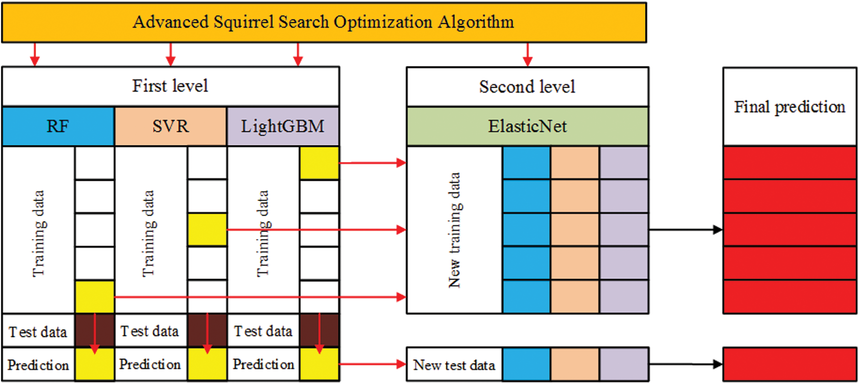
Figure 1: The proposed optimized two-level ensemble model
The dataset employed in this research consists of 10 features used to describe the design parameters of metamaterial antenna; 9 features of them are employed to estimate the optimal antenna’s bandwidth using the proposed model. The most significant features in this dataset are described in Tab. 2. The dataset is freely available on Kaggle [36] and is composed of 572 records. Each record consists of the following information about the metamaterial antenna: the distance between rings, the bandwidth of the antenna, the width and height of the split ring resonator, the gap between the rings, the width of the rings, the number of split-ring resonator cells in the array, the distance between the antenna patch and the array, the gain value, the return loss, and the distance between split-ring resonator cells in the array. In this research, 10 features are used to train the regression model, and the 10th feature, the bandwidth of the metamaterial antenna, can be optimally predicted using the proposed two-level ensemble model.

The graphical analysis of the dataset features is depicted in Fig. 2. In this figure, the distributions histograms of the feature are presented. In addition, the Pearson coefficient is calculated for each feature as shown in the figure. The large Pearson coefficient refers to the close correlation between the feature in the x-axis and the feature on the y-axis. In addition, it can be noted from the figure that the features namely Ya and Xa are highly correlated with the antenna bandwidth, whereas the features namely Wm and Tm are slightly correlated with the antenna bandwidth.
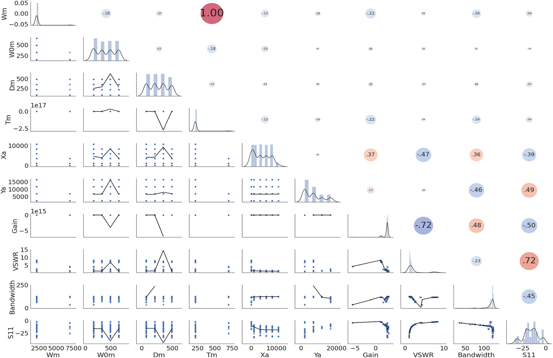
Figure 2: Analysis of the features of the metamaterial antenna dataset
The statistical analysis of the dataset features is presented in Tab. 3. This analysis is measured in terms of the count of records of the dataset, the mean and standard deviation of each feature, and the minimum and maximum values. As shown in the table, there are features with very small values and other features with very large values. Therefore, scaling the values of all features is necessary to properly balance the effect of each feature on the trained regression model. In addition, the mean of the features is varying differently, therefore, it is necessary to scale the values of these features. To realize this, the min-max scalar is adopted to make the values of all the features reside in the same range based on the following equation.
where

Random forest (RF) is a machine learning algorithm based on ensemble learning and can be used for regression and classification tasks. It belongs to the class of supervised machine learning algorithms. The underlying method used in random forests is the bagging technique in which a set of trees is constructed in parallel to form the random forest architecture. While building the trees of the random forest, no interaction is performed between these trees. At the training stage of this approach, a multitude of decision trees is constructed to be used in either classification or regression. In the case of regression tasks, the output of random forest is the mean prediction of the individual trees. Therefore, the prediction using random forest is considered a combination of the multiple predictions achieved by the constructed decision trees [37].
Support vector regression (SVR) is one of the applications of support vector machines (SVM), which is firstly introduced in 1954. Structural minimization and statistical learning theory are the basic principles of SVM. The SVR model is used to predict values in a dataset based on the following equation.
where
2.4 Light Gradient Boosting Machine
Light gradient boosting machine (LightGBM) is a regression model based on reducing the dimension of the data for adaptation and increasing the speed of the regression process. In addition, this model is optimized using the direct support for categorical features, acceleration of histogram difference, a leaf-wise leaf growth strategy with depth limitation, and a decision tree algorithm based on a histogram. Moreover, this model is distinguished by the rapid processing of massive datasets, distributed support and good accuracy, low memory consumption, fast training speed, and supporting parallel training with high efficiency [39].
ElasticNet regression model is one of the modern machine learning models that target finding the best coefficients that minimize the sum of error squares. It is based on applying a penalty to these coefficients until finding the best values. The critique on the well-known Lasso regression model was the main inspiration for the emergence of this approach. In the Lasso model, the variable selection is unstable as it depends mainly on the dataset. Therefore, the ElasticNet model presents a novel solution by combining the penalties of Lasso and Ridge models to utilize the advantages of both. This results in an efficient smoothing of the prediction curve. In addition, in the ElasticNet approach, the number of variables, for high dimensional data, is included in the training procedure. In the case of variables in highly correlated groups, ElasticNet takes a sufficient number of variables to cover these groups [40].
2.6 Advanced Squirrel Search Optimization Algorithm
To get the best performance of the employed regression models, a search space is constructed based on the potential values of the hyper-parameters of each regression model. The hyper-parameters of this search space are presented in Tab. 4. The constructed search space is searched using the advanced squirrel search optimization algorithm (ASSOA) that is recently emerged in the literature [41]. The basic idea of this algorithm is based on the flying squirrel’s search process. The algorithm employs three kinds of trees that are used by squirrels in moving between them. The trees representing the optimal solution are referred to as hickory trees. The trees representing the near-optimal solution are referred to as oak trees. The trees representing the non-optimal solution are referred to as normal trees. The advantage of ASSOA over the traditional squirrel search optimized algorithm is that it adds additional movements among the trees to reach the best solution more efficiently. These movements include exponential, diagonal, horizontal, and vertical movements as shown in Fig. 3. In addition, the velocities and locations of these movements are represented by the following equations.
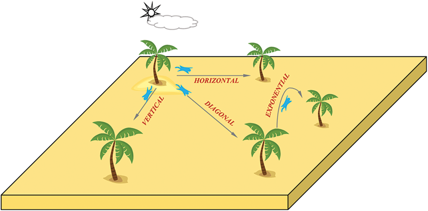
Figure 3: The movements of flying squirrels in the advanced squirrel search optimization algorithm [41]
where Vi,j and Fi,j denote the velocity and location of the ith squirrel in the jth dimension, for i value ranges from 1 to n and j value ranges from 1 to d. The initial locations of the squirrels are set to random values from a uniform distribution. The fitness function is then calculated for each flying squirrel to search for the optimal solutions in the search space. For more details about the employed ASSOA algorithm, please refer to [41].
2.7 The Proposed Two-Level Ensemble Model
After optimizing the parameters of each regression model in the proposed ensemble, these optimized models are integrated into a unified two-level ensemble. The first level in this ensemble consists of three regression models, namely SVR, RF, and LightGBM models, whereas the second level consists of the ElasticNet regression model. Algorithm 1 depicts the operation of the proposed ensemble model. Where L1, …, LT, and L denote the T models in the first level and the single model in the second level of the ensemble, respectively. The final output of the ensemble model, denoted by H(x), is the optimal predicted bandwidth value that best matches the input features of the metamaterial antenna.

To evaluate the performance of the proposed two-level ensemble model, the ASSOA algorithm is employed to find the best values of the hyper-parameters for each single regression model in the two levels of the ensemble. Tab. 4 depicts the search space for each hyper-parameter along with the best values retrieved, by the ASSOA algorithm, from the search space that achieve the best prediction results for each regression model separately. On the other hand, a set of evaluation metrics is employed to measure the regression models’ performance. These metrics are presented in Tab. 5 and include root mean squared error (RMSE), mean absolute error (MAE), mean bias error (MBE), and R2. In these metrics,

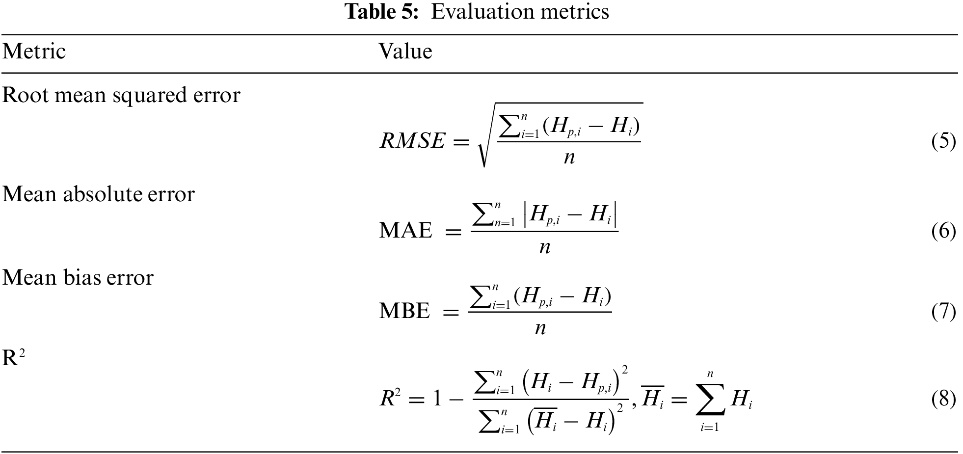
Fig. 4 depicts the prediction results of the training and testing sets based on the separate application of the regression models along with the proposed two-level ensemble model. As shown in the figure, the proposed approach achieves the best value of the R2 metric (0.9905) for the testing set. However, R2 values of RF, SVR, and LightGBM are (0.9854), (0.9764), and (0.9768), respectively. These values show the superiority of the proposed approach in generalizing the prediction of the antenna bandwidth.
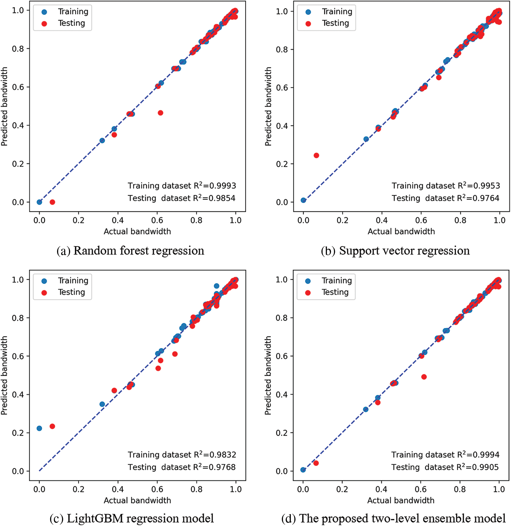
Figure 4: The prediction results of the training and testing sets based on the regression models
As the proposed approach is based on fine-tuning the results of the individual regression models using the second level of regression, the results show the ability of this approach to achieve generalization better than the separate application of the regression models. To demonstrate this achievement, Fig. 5 presents the prediction results of the testing sets based on RMSE and R2 metrics. As shown in the figure, the proposed approach could achieve the smallest RMSE value while keeping the value of R2 higher than the other models, which reflects the effectiveness of the proposed approach in predicting the bandwidth values and generalizing the prediction task.
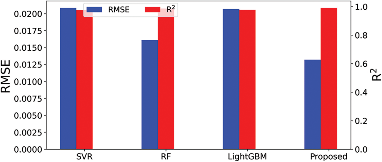
Figure 5: RMSE and R2 values of the different models in the testing set
Fig. 6 shows the mapping between the predictions of the antenna bandwidth along with the corresponding actual values of the testing set using the proposed two-level ensemble model. It can be noted from this figure that the prediction results are close to the actual values, which proves the effectiveness of the proposed approach.
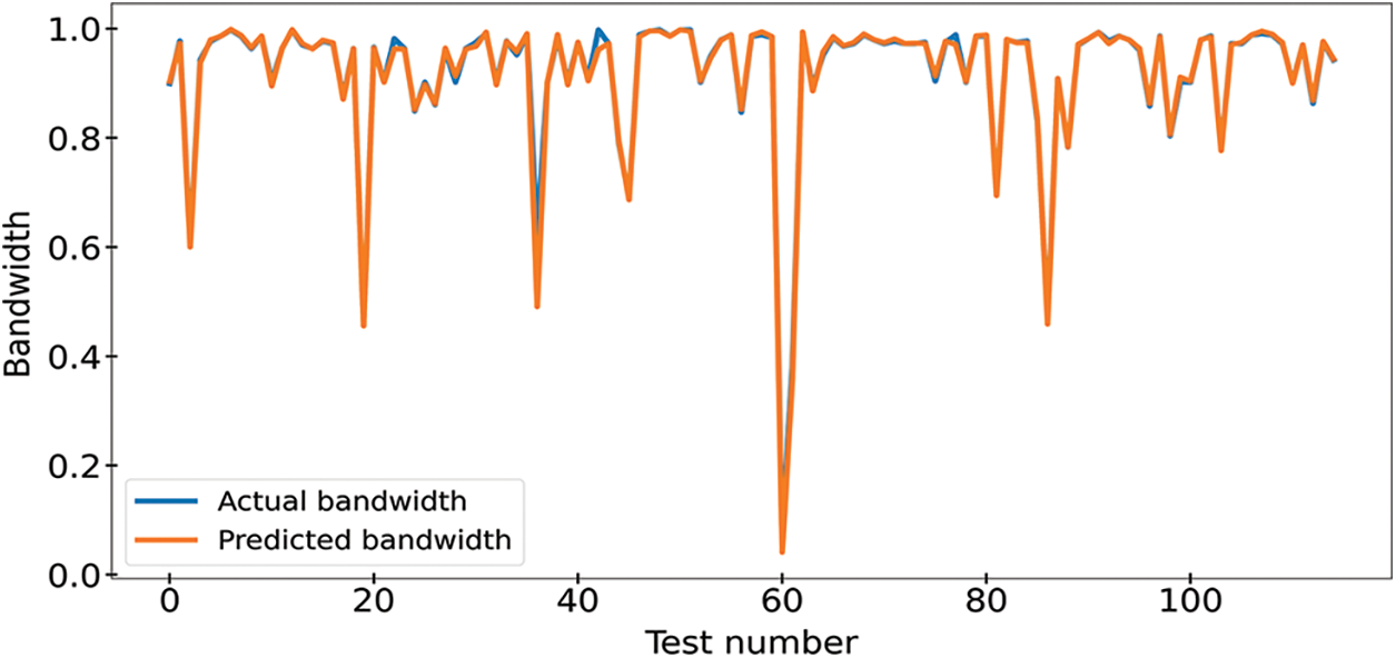
Figure 6: Actual and predicted bandwidth values of metamaterial antenna using the testing dataset
On the other hand, the prediction errors of the antenna bandwidth using SVR, RF, LightGBM, and the proposed approach are shown in Fig. 7. In this figure, the prediction error using LighGBM is the highest. However, the proposed approach could achieve the lowest prediction errors. These results emphasize the superiority of the proposed two-level ensemble model for the task of predicting the bandwidth of metamaterial antenna.
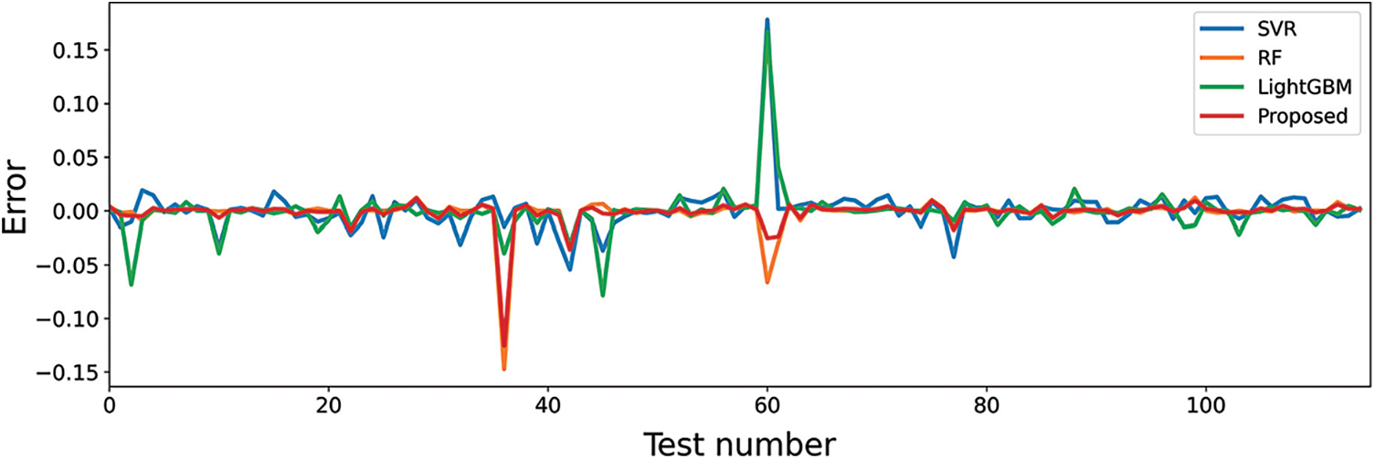
Figure 7: Error in predicting the bandwidth values of metamaterial antenna using the testing dataset
To further investigate the effective features contributing to the achieved results, Fig. 8 depicts the significant features based on the RF and LightGBM regression models. As the best kernel function adopted to this task is ‘rbf’, finding out the significance of the features is not available. As shown in this figure, the most significant features are the Gain, Ya, VSWR, S11, Xa, W0m, and Dm. These features match the previous analysis applied to the features as depicted in the Pearson values of Fig. 2, where the high correlation between these features and the bandwidth of the metamaterial antenna are represented by high values of Pearson coefficients.
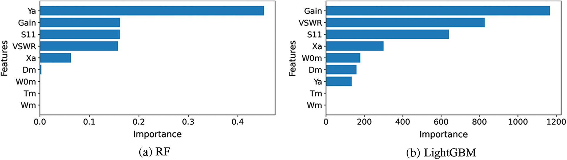
Figure 8: Feature importance of the regression models
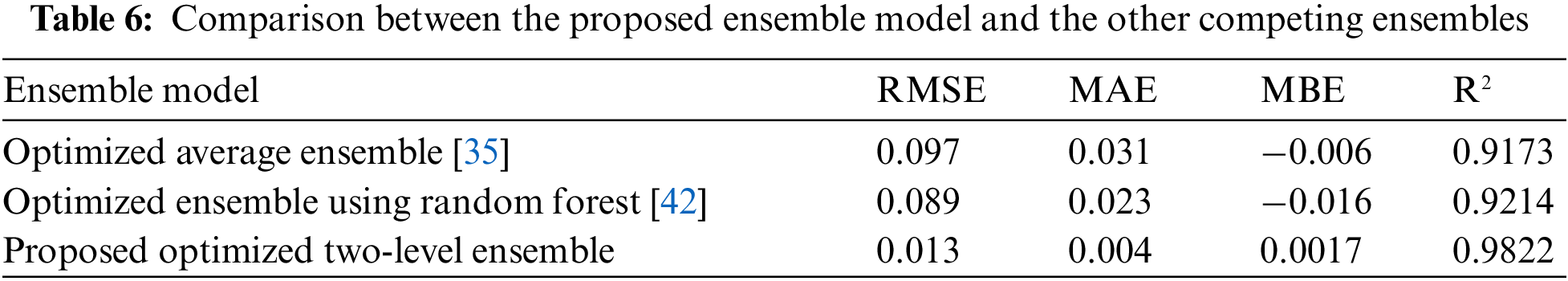
To emphasize the superiority of the proposed two-level ensemble model, we compared it with other ensemble models that are recently published in the literature and target the same task of predicting the bandwidth of metamaterial antenna based on the same dataset. Tab. 6 presents a comparison between the proposed ensemble model and two other ensemble models. As shown in the table, the measured values of the evaluation metrics calculated from the achieved results using the proposed approach outperform those of the other competing approaches. In specific, the achieved RMSE using the proposed approach is (0.013) which is better than the achieved RMSE by the other approaches (0.097 and 0.089). In addition, the MAE value achieved by the proposed model is (0.004) is better than the MAE values of the competing approaches (0.031 and 0.023). In addition, the value of MBE achieved by the proposed approach is (0.0017) which reflects that the mean value of differences between predicted and true values is smaller than the achieved values by the other approaches (−0.006 and −0.016). Moreover, the value of R2 achieved by the proposed approach (0.09822) is better than the achieved values by the competing approaches, which emphasized the effectiveness of the proposed approach in predicting the bandwidth of metamaterial antennas.
In this research, we addressed the problem of accurately predicting the bandwidth of metamaterial antenna. The solution presented in this paper is expressed in terms of a novel two-level ensemble model based on three machine learning regression models in the first level namely, random forest, support vector regression, and light gradient boosting machine. The integration of these models into a unified ensemble model is performed in terms of another regression model namely, ElasticNet located in the second level of the ensemble. The role of the second level is to combine the values of the models in the first level to train the ElasticNet model. The advanced squirrel search optimization algorithm is used to find the best hyper-parameters of the four regression models employed in the two levels of the proposed ensemble. The proposed ensemble model is evaluated in terms of a freely available benchmark dataset that contains a set of features describing various designs of metamaterial antennas along with the corresponding target bandwidth value. Experimental results showed that the proposed optimized two-level ensemble model outperforms two other ensemble models that are recently published in the literature that address the same task. The results based on four evaluation criteria emphasized the superiority of the proposed approach.
Acknowledgement: The authors extend their appreciation to the Deputyship for Research & Innovation, Ministry of Education in Saudi Arabia for funding this research work through the project number (IFP2021-033).
Funding Statement: The authors received funding for this study from the Deputyship for Research & Innovation, Ministry of Education in Saudi Arabia for funding this research work through the project number (IFP2021-033).
Conflicts of Interest: The authors declare that they have no conflicts of interest to report regarding the present study.
1. H. Misilmani and T. Naous, “Machine learning in antenna design: An overview on machine learning concept and algorithms,” in Int. Conf. on High-Performance Computing & Simulation, Dublin, Ireland, pp. 600–607, 2019. [Google Scholar]
2. C. Gianfagna, H. Yu, M. Swaminathan, R. Pulugurtha, R. Tummala et al., “Machine-learning approach for design of nanomagnetic based antennas,” Journal of Electronic Materials, vol. 46, no. 1, pp. 4963–4975, 2017. [Google Scholar]
3. S. Ghoneim, T. Farrag, A. Rashed, E. El-Kenawy and A. Ibrahim, “Adaptive dynamic meta-heuristics for feature selection and classification in diagnostic accuracy of transformer faults,” IEEE Access, vol. 9, no. 1, pp. 78324–78340, 2021. [Google Scholar]
4. L. Yuan, X. Yang, C. Wang and B. Wang, “Multi-branch artificial neural network modeling for inverse estimation of antenna array directivity,” IEEE Transactions on Antennas and Propagation, vol. 68, no. 6, pp. 4417–4427, 2020. [Google Scholar]
5. A. Ibrahim, S. Mirjalili, M. El-Said, S. Ghoneim, M. Alharthi et al., “Wind speed ensemble forecasting based on deep learning using adaptive dynamic optimization algorithm,” IEEE Access, vol. 9, no. 1, pp. 1–18, 2021. [Google Scholar]
6. B. Zhou and D. Jiao, “Direct finite element solver of linear complexity for analyzing electrically large problems,” in Int. Review of Progress in Applied Computational Electromagnetics, Williamsburg, VA, USA, pp. 1–2, 2015. [Google Scholar]
7. A. Kumar and M. Singh, “Band-notched planar UWB microstrip antenna with T-shaped slot,” Radioelectronics and Communications Systems, vol. 40161, no. 8, pp. 371–376, 2018. [Google Scholar]
8. R. Verma and D. Srivastava, “Bandwidth enhancement of a slot-loaded T-shape patch antenna,” Journal of Computational Electronics, vol. 18, no. 1, pp. 205–210, 2019. [Google Scholar]
9. R. Verma and D. Srivastava, “Design, optimization and comparative analysis of T-shape slot loaded microstrip patch antenna using PSO,” Photonic Network Communications, vol. 38, no. 1, pp. 343–355, 2019. [Google Scholar]
10. E. El-kenawy, H. Abutarboush, A. Mohamed and A. Ibrahim, “Advance artificial intelligence technique for designing double T-shaped monopole antenna,” Computers Materials & Continua, vol. 69, no. 3, pp. 2983–2995, 2021. [Google Scholar]
11. E. El-Kenawy, S. Mirjalili, S. Ghoneim, M. Eid, M. El-Said et al., “Advanced ensemble model for solar radiation forecasting using sine cosine algorithm and Newton’s laws,” IEEE Access, vol. 9, no. 1, pp. 115750–115765, 2021. [Google Scholar]
12. H. El Misilmani, T. Naous and S. Al-Khatib, “A review on the design and optimization of antennas using machine learning algorithms and techniques,” International Journal of RF and Microwave Computer-Aided Engineering, vol. 30, no. 10, pp. 1–28, 2020. [Google Scholar]
13. J. Song, J. Zhao, F. Dong, J. Zhao, Z. Qian et al., “A novel regression modeling method for PMSLM structural design optimization using a distance-weighted KNN algorithm,” IEEE Transactions on Industry Applications, vol. 54, no. 5, pp. 4198–4206, 2018. [Google Scholar]
14. J. Song, F. Dong, J. Zhao, H. Wang, Z. He et al., “An efficient multi-objective design optimization method for a PMSLM based on an extreme learning Machine,” IEEE Transactions on Industrial Electronics, vol. 66, no. 2, pp. 1001–1011, 2019. [Google Scholar]
15. P. Arnoux, P. Caillard and F. Gillon, “Modeling finite-element constraint to run an electrical machine design optimization using machine learning,” IEEE Transactions on Magnetics, vol. 51, no. 3, pp. 1–4, 2015. [Google Scholar]
16. H. Li, L. Cui, Z. Ma and B. Li, “Multi-objective optimization of the Halbach array permanent magnet spherical motor based on support vector machine,” Energies, vol. 13, no. 1, pp. 5704–5720, 2020. [Google Scholar]
17. J. Zhao, J. Huang, Y. Wang and K. Liu, “Design optimization of permanent magnet synchronous linear motor by multi-SVM,” in Proc. of the Int. Conf. on Electrical Machines and Systems (ICEMS), Hangzhou, China, pp. 1279–1282, 2014. [Google Scholar]
18. X. Sun, J. Wu, G. Lei, Y. Cai, X. Chen et al., “Torque modeling of a segmented-rotor SRM using maximum-correntropy criterion-based LSSVR for torque calculation of EVs,” IEEE Journal of Emerging and Selected Topics in Power Electronics, vol. 9, no. 3, pp. 2674–2684, 2020. [Google Scholar]
19. J. Wu, X. Sun and J. Zhu, “Accurate torque modeling with PSO-based recursive robust LSSVR for a segmented-rotor switched reluctance motor,” CES Transactions on Electrical Machines and Systems, vol. 4, no. 2, pp. 96–104, 2020. [Google Scholar]
20. A. Khan, M. Mohammadi, V. Ghorbanian and D. Lowther, “Efficiency map prediction of motor drives using deep learning,” IEEE Transactions on Magnetics, vol. 56, no. 3, pp. 1–4, 2020. [Google Scholar]
21. W. Kirchgassner, O. Wallscheid and J. Bocker, “Deep residual convolutional and recurrent neural networks for temperature estimation in permanent magnet synchronous motors,” in Proc. of the IEEE Int. Electric Machines & Drives Conf. (IEMDC), San Diego, CA, USA, pp. 1439–1446, 2019. [Google Scholar]
22. W. Kirchgassner, O. Wallscheid and J. Boecker, “Estimating electric motor temperatures with deep residual machine learning,” IEEE Transactions on Power Electronics, vol. 36, no. 7, pp. 7480–7488, 2021. [Google Scholar]
23. A. Khan, V. Ghorbanian and D. Lowther, “Deep learning for magnetic field estimation,” IEEE Transactions on Magnetics, vol. 55, no. 6, pp. 1–4, 2019. [Google Scholar]
24. Q. Wu, Y. Cao, H. Wang and W. Hong, “Machine-learning-assisted optimization and its application to antenna designs: Opportunities and challenges,” China Communications, vol. 17, no. 4, pp. 152–164, 2020. [Google Scholar]
25. C. Maeurer, P. Futter and G. Gampala, “Antenna design exploration and optimization using machine learning,” in Proc. of European Conf. on Antennas and Propagation, Copenhagen, Denmark, pp. 1–5, 2020. [Google Scholar]
26. A. Massa, D. Marcantonio, X. Chen, M. Li and M. Salucci, “DNNs as applied to electromagnetics: Antennas, and propagation- A Review,” IEEE Antennas and Wireless Propagation Letters, vol. 18, no. 11, pp. 2225–2229, 2019. [Google Scholar]
27. L. Cui, Y. Zhang, R. Zhang and Q. Liu, “A modified efficient KNN method for antenna optimization and design,” IEEE Transactions on Antennas and Propagation, vol. 68, no. 10, pp. 6858–6866, 2020. [Google Scholar]
28. J. Li, W. Water, B. Zhu and J. Lu, “Integrated high-frequency coaxial transformer design platform using artificial neural network optimization and FEM simulation,” IEEE Transactions on Magnetics, vol. 51, no. 3, pp. 1–4, 2015. [Google Scholar]
29. H. Sasaki and H. Igarashi, “Topology optimization accelerated by deep learning,” IEEE Transactions on Magnetics, vol. 55, no. 6, pp. 1–5, 2019. [Google Scholar]
30. S. Doi, S. H. Sasaki and H. Igarashi, “Multi-objective topology optimization of rotating machines using deep learning,” IEEE Transactions on Magnetics, vol. 55, no. 6, pp. 1–5, 2019. [Google Scholar]
31. J. Asanuma, S. Doi and H. HIgarashi, “Transfer learning through deep learning: Application to topology optimization of electric motor,” IEEE Transactions on Magnetics, vol. 56, no. 3, pp. 1–4, 2020. [Google Scholar]
32. S. Barmada, N. Fontana, L. Sani, D. Thomopulos and M. Tucci, “Deep learning and reduced models for fast optimization in electromagnetics,” IEEE Transactions on Magnetics, vol. 56, no. 3, pp. 1–6, 2020. [Google Scholar]
33. W. Wang, J. Zhao, Y. Zhou and F. Dong, “New optimization design method for a double secondary linear motor based on R-DNN modeling method and MCS optimization algorithm,” Chinese Journal of Electrical Engineering, vol. 6, no. 3, pp. 98–105, 2020. [Google Scholar]
34. Y. M. You, “Multi-objective optimal design of permanent magnet synchronous motor for electric vehicle based on deep learning,” Applied Sciences, vol. 10, no. 2, pp. 482–501, 2020. [Google Scholar]
35. A. Ibrahim, H. Abutarboush, A. Mohamed, M. Fouad and E. El-kenawy, “An optimized ensemble model for prediction the bandwidth of metamaterial antenna,” CMC-Computers, Materials & Continua, vol. 71, no. 1, pp. 199–213, 2022. [Google Scholar]
36. R. Machado, “Metamaterial Antennas,” 2019. [Online]. Available: https://www.kaggle.com/renanmav/metamaterial-antennas [Accessed:2022-1-20]. [Google Scholar]
37. Z. Zhou, Machine learning. Beijing: Tsinghua University Press, 2016. [Google Scholar]
38. R. Zhong, R. Johnson and Z. Chen, “Using machine learning methods to identify coals from drilling and logging-while-drilling LWD data,” in Proc. of Asia Pacific Unconventional Resources Technology Conf., Brisbane, Australia, pp. 1–10, 2019. [Google Scholar]
39. G. Ke, Q. Meng and T. Finley, “LightGBM: A highly efficient gradient boosting decision tree,” Advances in Neural Information Processing Systems, vol. 30, no. 1, pp. 3146–3154, 2017. [Google Scholar]
40. A. AlJawarneh, M. Ismail and A. Awajan, “ElasticNet regression and empirical mode decomposition for enhancing the accuracy of the model selection,” International Journal of Mathematical, Engineering and Management Sciences, vol. 6, no. 2, pp. 564–583, 2021. [Google Scholar]
41. E. El-Kenawy, S. Mirjalili, A. Ibrahim, M. Alrahmawy, M. El-Said et al., “Advanced meta-heuristics, convolutional neural networks, and feature selectors for efficient COVID-19 X-ray chest image classification,” IEEE Access, vol. 9, no. 1, pp. 36019–36037, 2021. [Google Scholar]
42. E. El-kenawy, A. Ibrahim, S. Mirjalili, Y. Zhang, S. Elnazer et al., “Optimized ensemble algorithm for predicting metamaterial antenna parameters,” CMC-Computers, Materials & Continua, vol. 71, no. 3, pp. 4989–5003, 2022. [Google Scholar]
 | This work is licensed under a Creative Commons Attribution 4.0 International License, which permits unrestricted use, distribution, and reproduction in any medium, provided the original work is properly cited. |