Computers, Materials & Continua DOI:10.32604/cmc.2022.027708
Article

On-line Recognition of Abnormal Patterns in Bivariate Autocorrelated Process Using Random Forest

Miao Xu1, Bo Zhu1,*, Chunmei Chen1 and Yuwei Wan2

1College of Mechanical and Electrical Engineering, Kunming University of Science & Technology, Kunming, 650500, China
2School of Engineering, Cardiff University, Cardiff, CF24 3AA, UK
*Corresponding Author: Bo Zhu. Email: zhubo20110720@163.com
Received: 24 January 2022; Accepted: 08 March 2022

Abstract: It is not uncommon that two or more related process quality characteristics are needed to be monitored simultaneously in production process for most of time. Meanwhile, the observations obtained online are often serially autocorrelated due to high sampling frequency and process dynamics. This goes against the statistical I.I.D assumption in using the multivariate control charts, which may lead to the performance of multivariate control charts collapse soon. Meanwhile, the process control method based on pattern recognition as a non-statistical approach is not confined by this limitation, and further provide more useful information for quality practitioners to locate the assignable causes led to process abnormalities. This study proposed a pattern recognition model using Random Forest (RF) as pattern model to detect and identify the abnormalities in bivariate autocorrelated process. The simulation experiment results demonstrate that the model is superior on recognition accuracy (RA) (97.96%) to back propagation neural networks (BPNN) (95.69%), probability neural networks (PNN) (94.31%), and support vector machine (SVM) (97.16%). When experimenting with simulated dynamic process data flow, the model also achieved better average running length (ARL) and standard deviation of ARL (SRL) than those of the four comparative approaches in most cases of mean shift magnitude. Therefore, we get the conclusion that the RF model is a promising approach for detecting abnormalities in the bivariate autocorrelated process. Although bivariate autocorrelated process is focused in this study, the proposed model can be extended to multivariate autocorrelated process control.

Keywords: Random Forest; bivariate autocorrelated process; pattern recognition; average run length

1  Introduction

Statistical Process Control (SPC) provides a series of control charts for monitoring production processes, which have become the core of the six-sigma management. The SPC control charts are aimed at distinguishing whether a process is running in its intended mode or not, to improve the process performance and maintain an efficient production process. It is not uncommon that two or more related process quality characteristics are needed to be monitored simultaneously in production process for most of time, namely the multivariate process. The multivariate control charts, for example Hotelling’s T2 chart [1], multivariate cumulative sum (MCUSUM) [2], and multivariate exponentially weighted moving average (MEWMA) [3], provide countermeasures for monitoring multivariate processes through constructing a synthetic statistic to distinguish whether a process state is out of control or not. However, two inherent issues exist in using of multivariate control charts. The first issue is, multivariate control charts are theoretically based on the statistical assumption that the observations are independent and identically distributed (I.I.D) [4]. Nevertheless, the observations obtained online are often serially autocorrelated due to high sampling frequency and process dynamics in actual production process, especially in the continuous industries, such as smelting, chemical and food industry. This goes against the I.I.D assumption. Consequently, the performance of multivariate control charts would collapse soon, giving rise to serious false and missed alarms. The second issue is related to process diagnosis, that is, the synthetic statistics enable multivariate control charts to detect the abnormalities of process, but misses to provide details about the specific abnormal variables, which are considerably useful for locating the assignable reasons.

Two different kinds of solutions have been suggested to compensate the limitations of the traditional multivariate control charts. The first kind belongs to statistical approaches. In order to cope with the I.I.D issue, some scholars suggested directly adjusting control limits of control chart [5–7] or fitting a time-series model to the multivariate process and monitoring the forecast residuals [8–10]. The limit correcting measures can handle the problem of false and missed alarms to some extent, yet still follow the I.I.D assumption so can’t put things right once and for all. The residual measure overcomes successfully the I.I.D issue, whereas it is often difficult to fit an appropriate time-series model for multivariate process. A higher-order model may fit a process well, but brings heavier coefficient setting task at the same time, which throws higher requirements to practitioners’ experience and skill.

The second kind is to apply machine learning that stem from Artificial Intelligence to overcome the issues. The main idea is, to apply machine learning method to recognize patterns of process, and through that to detect process abnormalities and reveal abnormal variables. To do this well owes much to the excellent capabilities of classification and prediction of machine learning. Compared with statistical approaches, machine learning-based approaches completely escape from the I.I.D issue, and have no need of human involvement in practice. Thus, it is not merely a means of process quality control, but an effective way to achieve the intelligence in production.

Over the past several years, typical machine learning approaches have been implemented for pattern recognition in the process quality control, including artificial neural networks (ANNs) [11–14], Bayesian networks [15], decision trees (DTs) [16], fuzzy approaches [17,18], support vector machine (SVM) [19–25], etc. Among those, ANN, DT and SVM are most used, however suffer from many weaknesses. For instance, the recognition accuracy of ANNs depends on a large amount of training data and a selective choice of lots of parameters. Failure to find the optimal parameters for an ANN model vastly affects its recognition accuracy. Another scandalous disadvantage of ANN is overfitting. Decision tree is not a kind of stable learning model, owing that a small change of the input data may leads to a completely different structure in training. Moreover, the overfitting issue also easily takes place in decision tree models. The recognition accuracy of SVM relies on a selective choice of the kernel function and corresponding parameters (e.g., cost parameter, slack variables and the margin of the hyperplane), and that is not an easy thing.

According to the literature, there are already a lot of researches on application of machine learning approaches in univariate process, which is independent or autocorrelated, and non-autocorrelated multivariate process, while only a few cases could be found concerning the autocorrelated multivariate processes [26–28]. Generally speaking, when it comes to choosing a better machining learning approach for a certain problem, the background of the problem itself plays a crucial role. Therefore, the investigative significance of trying new machine learning methods in established problem domain should never be underestimated. It is the same for the monitoring of autocorrelated multivariate process.

Random forest (RF), as a type of bagging ensemble learning method [29], has many advantages, such as a quick training speed, a robust anti-overfitting ability, and an easy implementation that requires determining only very few parameters, in addition to being easily parallelizable, etc., so has been widely used in pattern classification and prediction [30–33]. RF has also been introduced into the process quality control field in recent years. Zhu et al. [34] proposed a RF based recognition model for the eight classic patterns in autocorrelated univariate process, and reported to have achieved a not bad recognition accuracy (94.98% and 91.25% for positive and negative autocorrelation respectively). Wan et al. [35] used a PSO-optimized RF in recognition of abnormal patterns in bivariate autocorrelated process, and achieved good off-line recognition performance.

Inspired by that, this study established a model using RF for on-line recognition of abnormal patterns in bivariate autocorrelated process. In order to evaluate the performance of the proposed model, it was firstly compared with three other commonly used machine learning methods, i.e., BPNN, PNN, SVM, on RA. Then, its ARLs and SRLs in case of different mean shift magnitudes are obtained from simulated process data flows, and compared with those of BPNN, PNN, SVM and Z control chart. All experiment results demonstrate that the proposed model has clear superiorities. Therefore, we think that our study presents a promising alternative approach for on-line recognition of abnormal patterns in bivariate autocorrelated process, which makes contribution to the process quality control field.

The rest of this paper is organized as follows. Section 2 describes the theoretical basis of bivariate autocorrelated process based on time series analysis. Section 3 demonstrates the abnormal patterns recognition model proposed. Then, some simulation experiments are conducted to verify the model and the results are discussed. Section 5 concludes this paper.

2  Bivariate Autocorrelated Process

According to literature, researches on multivariate process commonly choose bivariate process as the object to be without loss of generality, for it reflects the nature of multivariate process with low complexity. The AR (1) (first-order autoregressive) model is commonly used to model autocorrelated multivariate process for its lower complexity. Taking all these into account, we construct AR (1) model for bivariate autocorrelated process first and based on that to conduct our study.

The AR (1) model is expressed as follows.

[X1,tX2,t]=[μ1μ2]+[Φ1,1Φ1,2Φ2,1Φ2,2][X1,t−1X2,t−1]+[ε1,tε2,t](1)

or

Xt=μ+ΦXt−1+εt(2)

where, Xt=(X1,t,X2,t)T is a two dimensional quality characteristics vector observed at time t, in which, the X1 and X2 represent the two monitored quality characteristics variables respectively. i=1,2,…,t is the lag length, μT=(μ1,μ2) is the process mean vector, Φ=[Φ1,1Φ1,2Φ2,1Φ2,2]is the 1th autoregressive matrix, εtT=(ε1,t,ε2,t) represents a normal distributed fluctuation with zero-mean and covariance matrix Σ=[σ1,1σ1,2σ2,1σ2,2].

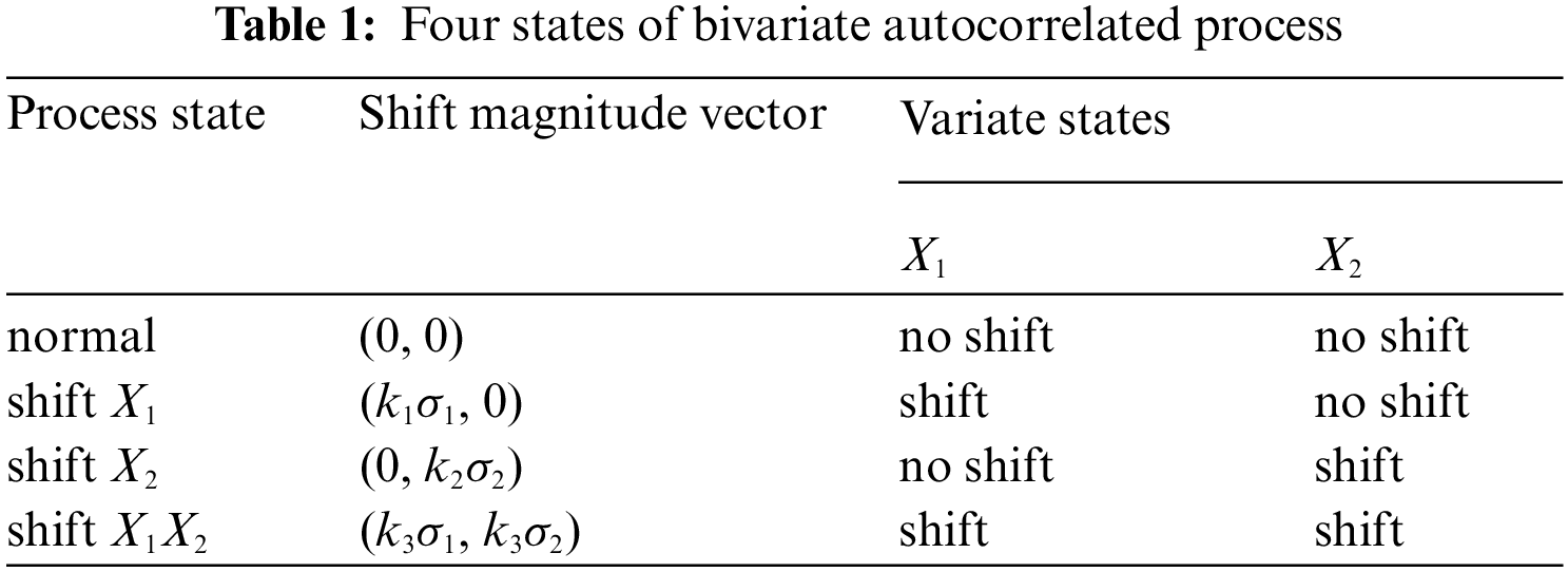
Eq. (1) describes a typical bivariate autocorrelated process in stationary state, in which the mean and variance are both constant. The production process is considered to be in control, which is called as normal state in our study, as it is in stationary state. However, the in-control state may changes to out-of-control state, which is called as abnormal state in our study, due to some assignable causes. According to the actual production process, the most common changes of process state from in-control to out-of-control manifest in process mean deviation. In order to introduce the deviation into the AR (1) model, the linear superposition method is used. Then, based on the Eq. (1), an abnormal state of the bivariate autocorrelated process has get as Eq. (3).

[X1,tX2,t]=[μ1μ2]+[Φ1,1Φ1,2Φ2,1Φ2,2][X1,t−1X2,t−1]+[ε1,tε2,t]+[k1σ1k2σ2](3)

or

Xt = μ+ΦXt−1+εt+k⊗σ(4)

where, σ=(σ1,σ2)T means process standard deviation vector, and k=(k1,k2)T means the times vector of mean shift magnitude in terms of σ. The symbol ⊗ is the Hadamard product, which means calculating the products of corresponding components of σ and k respectively.

To be corresponding to the values of k1 and k2 (equal to zero or not), the abnormal state can be divided into three types, namely, X1 deviated, X2 deviated and both two variables deviated. Hence, we have four patterns defined for a bivariate autocorrelated process in all, which are expressed as normal, shift X1, shift X2, shift X1X2 later in this paper. An abridged general view of the four patterns in bivariate autocorrelated process is shown in Fig. 1. In order to cover more scenarios of actual process, the value of k1 and k2 are set to be from 0 to 3, each indicating a different level of mean shift magnitude. In Tab. 1, the four patterns are listed in detail.

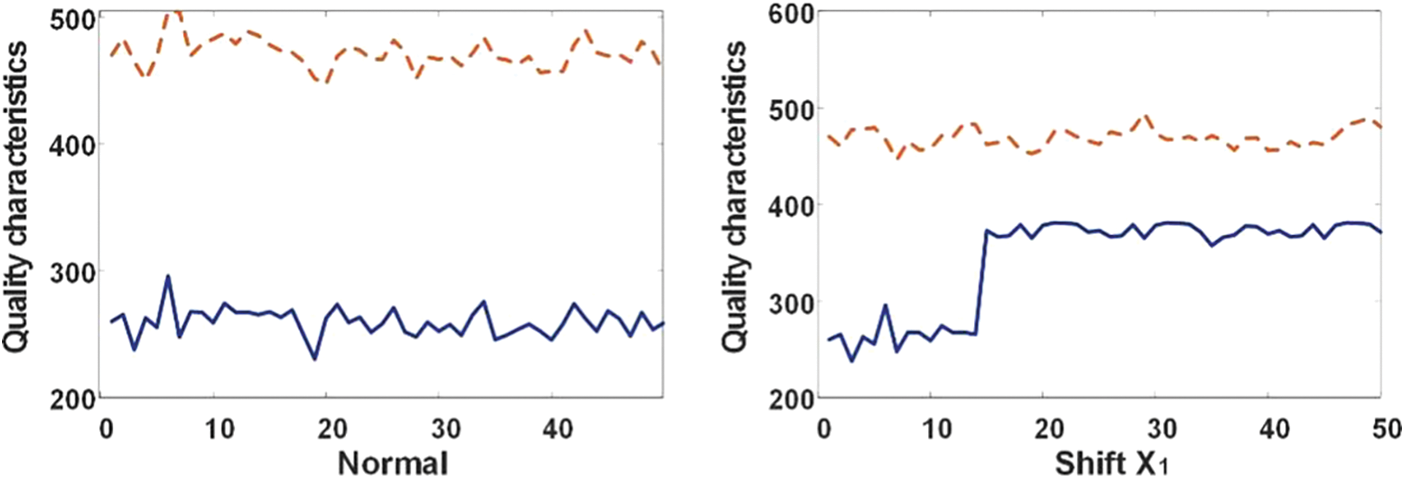
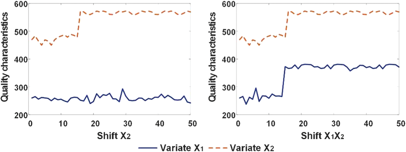
Figure 1: Four states of bivariate autocorrelated process

3  Needed Methods

3.1 The Classification Theory of RF

Random forest (RF) is a type of bagging ensemble learning model composed of a collection of improved decision trees. RF can be formally described as {h(X,Θk)|k=1,2,…,N}, where X represents the input pattern vector, and {Θk} represents the k-th decision tree trained with dataset randomly sampled from raw data set on bootstrap method. The improved decision tree as individual classifier is constructed through randomly choosing a set of features to be source of node segmentation in order to increase the diversity. The final classification result is obtained by way of most-voting on classifiers h1(X),h2(X),…,hN(X). Fig. 2 shows the schematic diagram of RF.

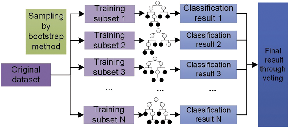
Figure 2: Schematic diagram of random forest classification algorithm

A simple deduction for the working principle of RF as follows [29]. A margin function is defined as

mg(X,Y)=avNI(hN(X)=Y)−maxj≠YavNI(hN(X)=j)(5)

where, I(⋅) is an indicator function and avN is to get the mean value. The margin function is used to calculate how many votes in average for the right class exceeds those for the other classes. A larger margin means that the classification can be given more confidence. So, the generalization error of RF can be obtained based on the margin as Eq. (6).

PE∗=PX,Y(mg(X,Y)<0)(6)

Eq. (6) demonstrates that {h(X,Θk)|k=1,2,…,N} obey the law of large numbers on condition that the value of N is large enough, i.e., there are plenty of trees are contained in the model. In addition, the upper limit of generalization of RF has been proved to be convergent as the random vectors Θ1,…,PE∗ convergent almost everywhere. It is given by

PX,Y(PΘ(h(X,Θ)=Y)−maxj≠YPΘ(h(X,Θ)=j)<0)(7)

Based on that, the upper limit of generalization error ε¯ can be defined as Eq. (8). Where, ρ¯  indicates the average correlation coefficient between trees, and s measures the average classification performance of the decision trees.

ε¯≤ρ¯(1−s2)s2(8)

It can be seen that the upper limit of generalization error become larger with the average correlation coefficient largen, and with the average classification performance becoming poorer. In other words, RF can or not achieve good overall performance depends on whether every tree perform as well as possible and whether there is large enough difference between trees.

There are commonly two approaches should be applied concurrently to enlarge difference between trees as follows: (a) in the aspect of data, generating different training data sets through resampling from the raw training data set to achieve different classifier; (b) in the aspect of model structure, each node of the individual tree is segmented with the optimum one of a feature subset randomly chosen from the entire feature set. In applying these two approaches, two parameters, i.e., ntree and mtry should be determined, of which the former is the quantity of trees, and the latter is the feature subset size.

In this study, the RF model for pattern classification is established by following 3 steps.

Step 1: ntree training sets Si{i=1,2,…,N} are achieved by Bootstrap sampling method from synthetic pattern sample data set generated by Mont Carlo simulation.

Step 2: equal number of trees are generated, with each one based on a training set Si. First, mtry features are randomly selected from the total feature set to construct the feature subset for each tree. Next, each tree begins splitting with the feature subset and growing to the possible greatest extent with no pruning.

Step 3: outputted class labels from each tree for a certain pattern sample is collected, and then the most voting method is used, namely, the number of votes for each class is added up to achieve the largest one, which is regarded as the classification result for the pattern sample.

3.2 The Proposed Model

In this section, we propose the RF-based model to recognize the four patterns in bivariate autocorrelated process. The framework of RF model is shown in Fig. 3.

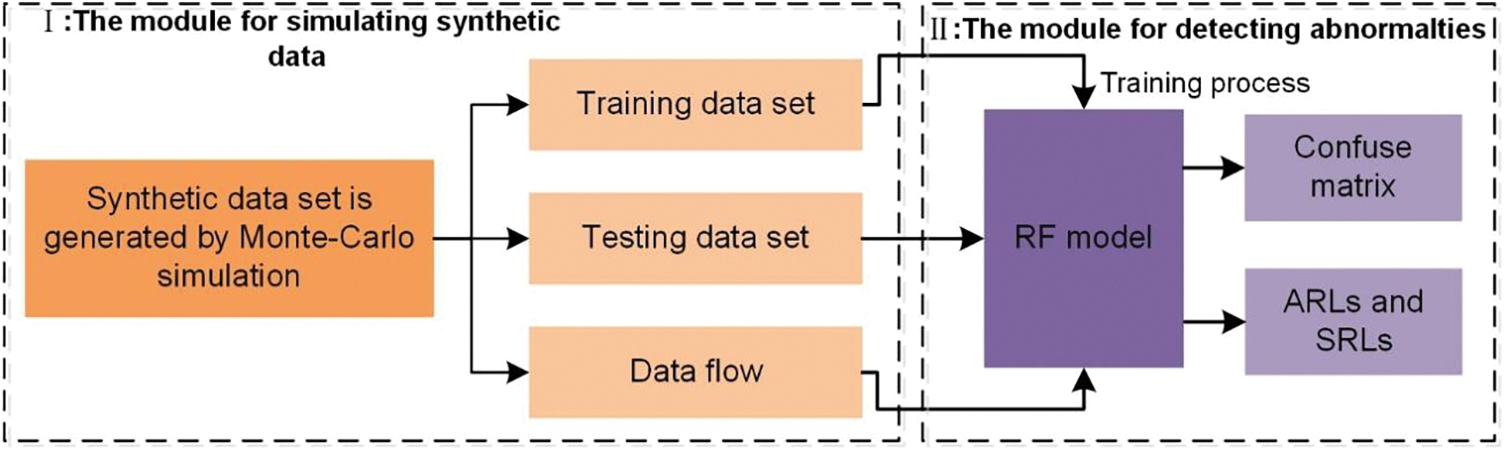
Figure 3: The framework of RF model

The model is composed of two sequential modules. In module I, the synthetic sample data set containing normal pattern and three abnormal patterns is generated through Monte-Carlo simulation method, and is divided into two distinct subsets, namely the training data set and the testing data set. In module Ⅱ, the RF model is trained through the training data set first, and the outputted confusion matrix is used as an evaluation index, indicating whether the RF should be retrained with adjusted key parameters (ntree, mtry). Then its classification generalization performance is attained with the testing data set if the two key parameters are confirmed. The well-trained RF is also used to detect abnormal patterns in process data flow, and its ARLs and SRLs are measured and calculated to evaluate its process monitoring performance.

3.3 Evaluation Method

A good process quality control procedure is one that, ensure a specific error rate (Type I error) when the process is still in-control, and detect the abnormalities quickly whenever the process is determined to be out-of-control. For that, ARL0 (in-control ARL) and ARL (out-of-control ARL) are commonly used as the indicators of process abnormality detecting performance. ARL0 is defined as the average number of samples have been taken before an in-control process is mis-alarmed by detector, and ARL is defined as the average number of samples that must be taken before the detector alarm since the process truly get out of control.

To evaluate the on-line detecting performance of the proposed model, its ARL0 and ARL are obtained from detecting simulated process and compared with those of some other process monitoring methods. Fig. 4 presents the detailed procedure of the evaluation for the proposed model. It is summarized as follows.

Off-line phase includes three steps as follows.

Step 1: Generate data of normal and abnormal patterns to construct training and testing dataset;

Step 2: Train the RF model with training dataset;

Step 3: Test the RF model with testing dataset, then the confuse matrix is attained for evaluating its generalization ability.

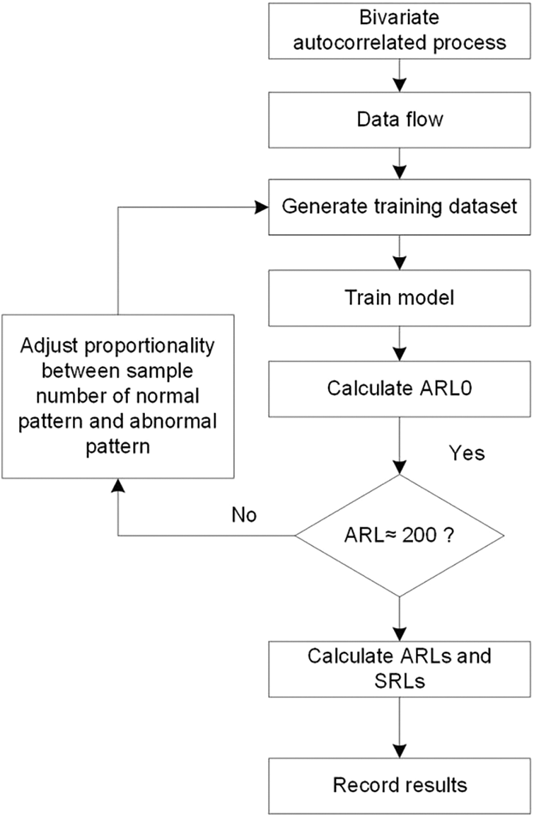
Figure 4: Running flow of proposed method for bivariate autocorrelated process

In order to simulate the fact that an actual process is in control before it get out of control, the shift point is set to be 51 for out-of-control data flow. Then, a moving sample window (the window size is 50, and moving step length is 1) is used to sample data from data flow and feed to the model till the model declare that an abnormality pattern is detected. The ARL0 is obtained by taken average of all in-control process data flow, making the head point as sampling start point, and the ARL is obtained by taken average of all out-of-control process data flow, making the shift point as sampling start point. On-line phase includes four steps as follows.

Step 1: A certain amount of process data flows, including in-control case and out-of-control cases with different magnitudes of mean shift, in which each case has 10000 samples, are generated by Mont-Carlo simulation method.

Step 2: Adjust proportionality between sample number of normal pattern and abnormal pattern in the training data set, and then train the RF model with the training data set.

Step 3: Apply the model to all in-control data flows to calculate ARL0. If ARL0 is around 200, go to step 4, else go to step 2;

Step 4: Apply the model to all types of out-of-control data flow to calculate ARLs and SRLs, and report the results.

4  Experiment Results and Discussion

In this section, simulation experiments processes and results are reported. All experiments are conducted in MATLAB 2018a on a PC with Intel Core i5-6200 CPU (2.30 GHz) and 4 GB memory. The RF is established on RF_MexStandalone-v0.02 toolbox.

4.1 Synthetic Raw Data Set Generation

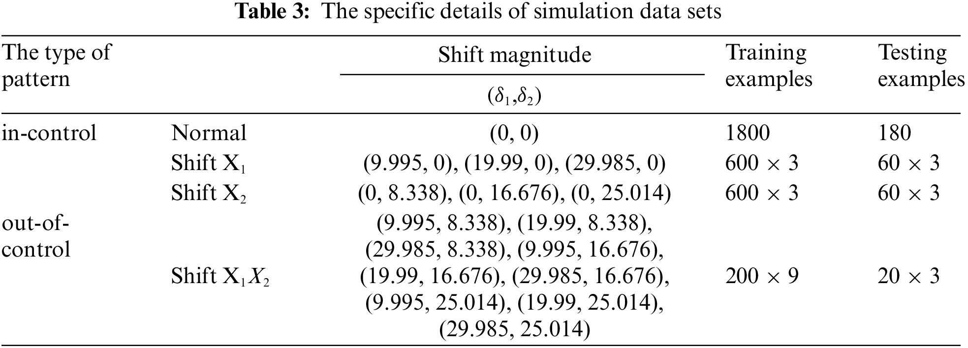
Ideally, abundant actual sample data should be acquired directly from practical production processes for training of model. However, it is costly in doing that. So, it has become a normal practice in researches in this field to generate enough synthetic samples of process through Monte-Carlo simulation method for training model. Training dataset and testing dataset of bivariate autocorrelated process as mentioned in Section 2 are generated first. In order to simulate the real bivariate autocorrelated process, six parameters are needed to be determined to reflect variation of fluctuation. Five of the parameters are assigned according to Fountoulaki et al. [27], including window size, bivariate mean vector, autoregressive matrix, covariance matrix and the magnitude of shift. The rest one (shift points of time) are reassigned to enhance the recognition accuracy of abnormal patterns, according to the result of one pre-experiment. The total parameters are shown in Tab. 2. More specifically, when the magnitude of one variable is set to be 1σ, 2σ and 3σ separately, the shift points are set to be 20, 30 and 40 respectively in shift X1 and shift X2. In particular, for shift X1X2, the shift points of two variables are set to be the same as the smaller mean shift magnitude, i.e., the shift points are set to be 20, when the mean shift magnitudes of variable X1 and variable X2 are set to be 1σ and 3σ separately.

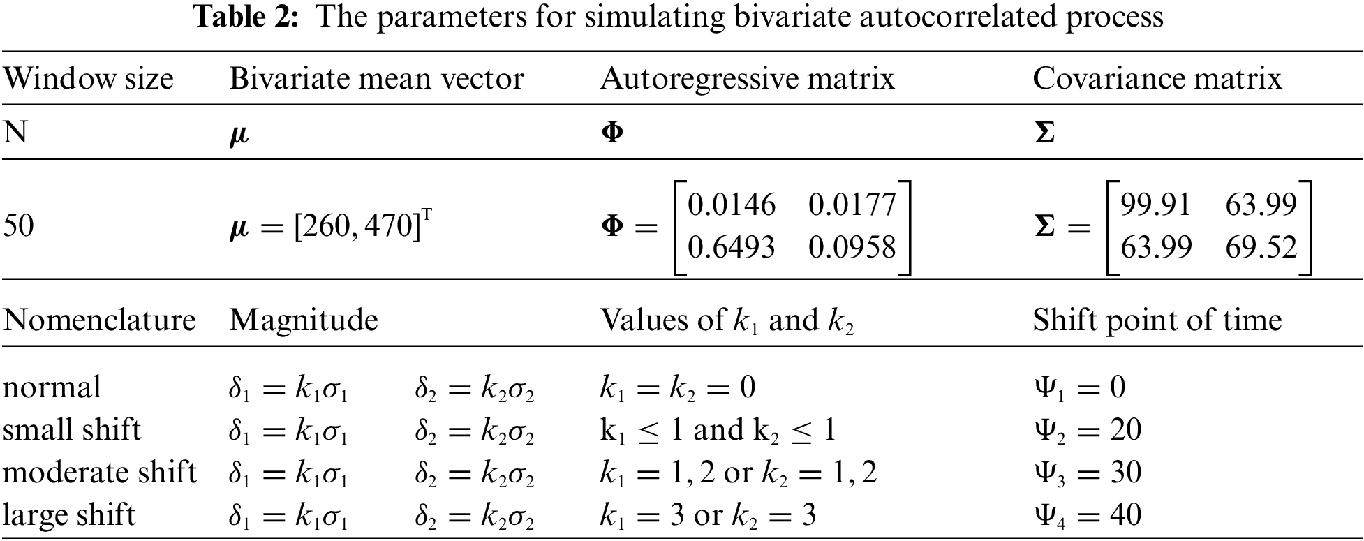
Fig. 5 presents the process of generating pattern samples. The generated training dataset and testing dataset are detailed in Tab. 3.

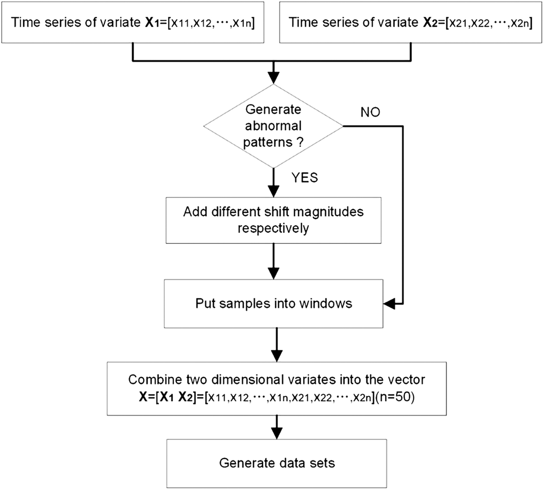
Figure 5: The process of patterns generation

4.2 Recognition Accuracy Comparison

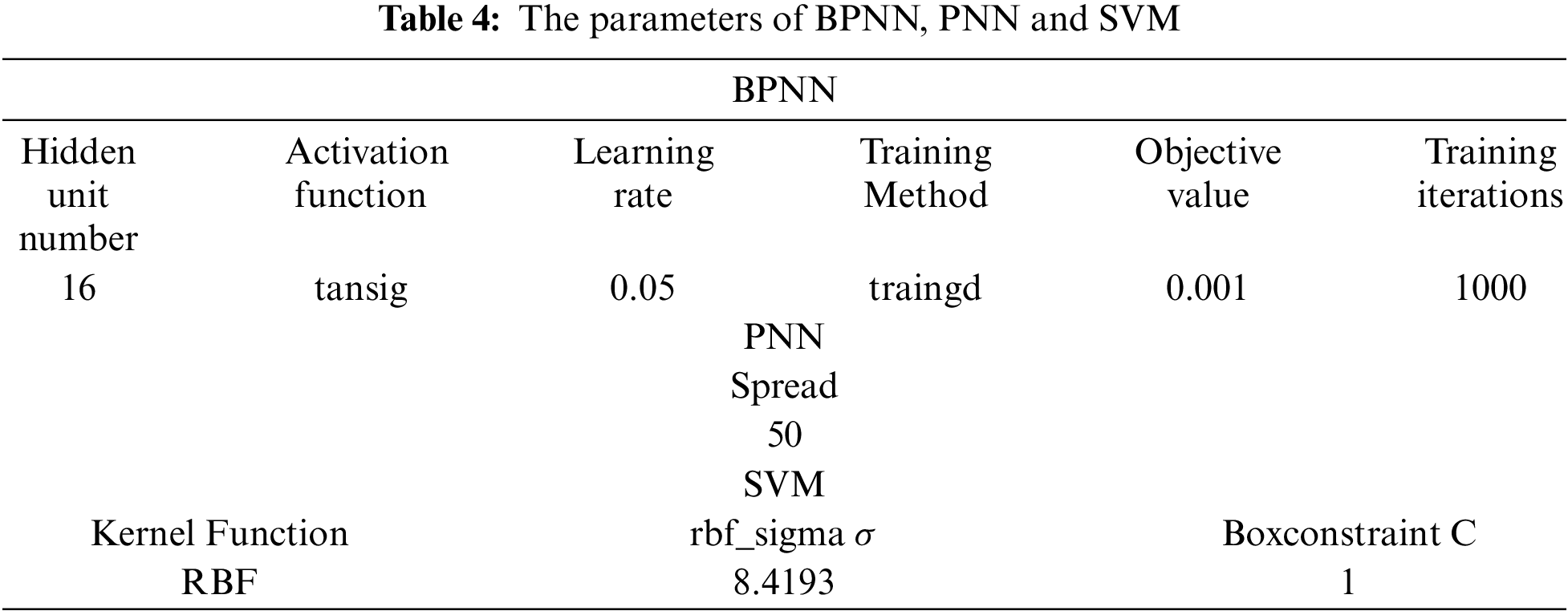
ANN and SVM are the most common approaches used to classify patterns in process quality control. For this reason, we conduct comparative experiments between our model and BPNN model, PNN model and SVM model respectively. The parameters of the BPNN, the PNN and the SVM are given in Tab. 4.

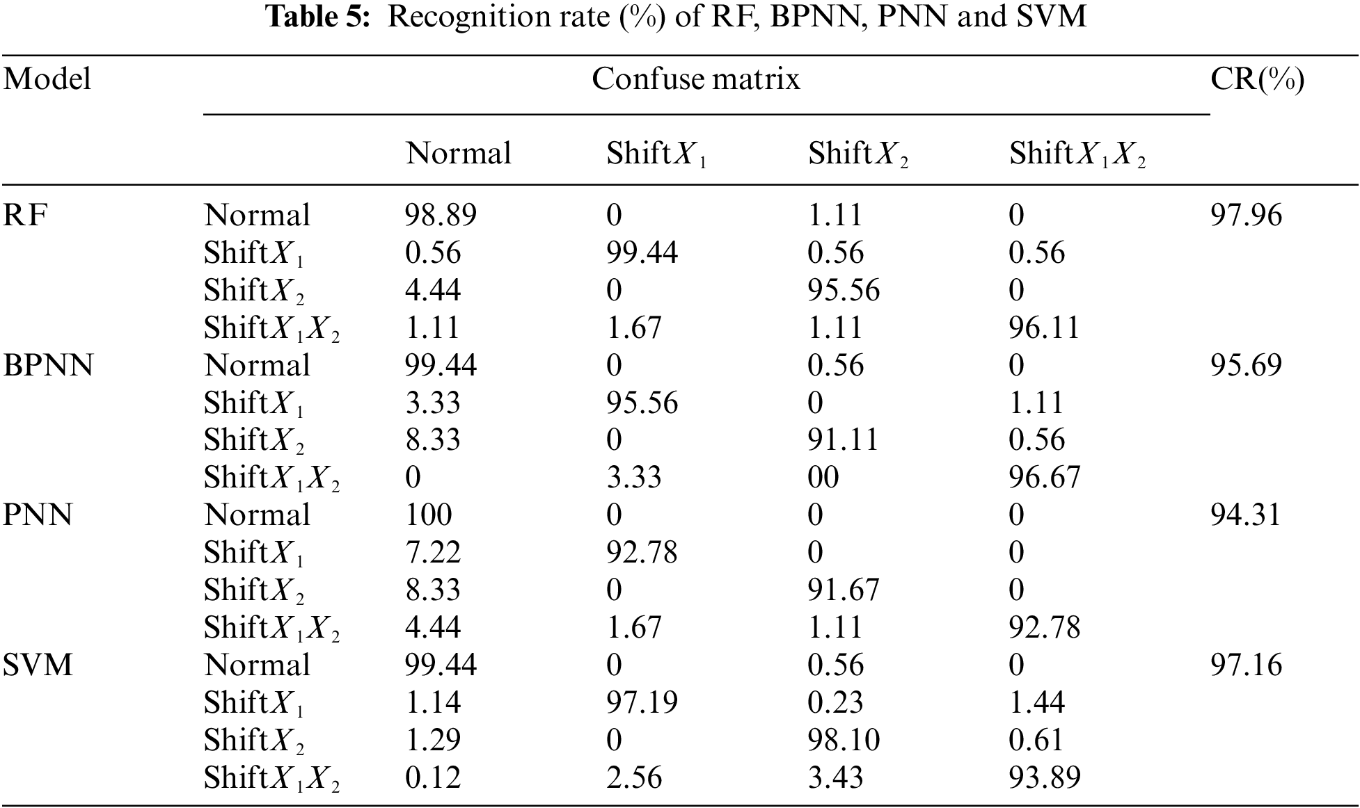
Tab. 5 demonstrates the recognition rate (%) of different models for bivariate autocorrelated process. From it, we can see that the RF model performs well for all the four patterns, and achieves the best RA (97.96%). The RA of the BPNN model reaches 95.96%, for its recognition accuracy of shift X2 attains only 91.11%. The PNN model gets the lowest RA (94.31%), since its recognition accuracies of three abnormal patterns are all lower than 93%. Although the SVM model performs well on two patterns (Normal and shift X2), which are even slightly higher than those of the RF model, it gets a slightly lower RA (97.16%), too.

Tab. 5 demonstrates the recognition rate (%) of different models for bivariate autocorrelated process. From it, we can see that the RF model performs well for all the four patterns, and achieves the best RA (97.96%). The RA of the BPNN model reaches 95.96%, for its recognition accuracy of shift X2 attains only 91.11%. The PNN model gets the lowest RA (94.31%), since its recognition accuracies of three abnormal patterns are all lower than 93%. Although the SVM model performs well on two patterns (Normal and shift X2), which are even slightly higher than those of the RF model, it gets a slightly lower RA (97.16%), too.

It appears that the proposed RF model perform best for off-line recognition in comparison with BPNN, PNN and SVM. More specifically, all of the four patterns are recognized finely, especially the X1X2 shift pattern. Additionally, it’s important not to neglect the much more experience needed for BPNN to determine a large number of model parameters, and the difficulties of SVM in solving multi classification problems. So, it can be considered that the proposed RF model is better than the other three models for off-line recognition of the bivariate autocorrelated process patterns.

4.3 ARLs Comparison

In this section, the performance of the proposed RF model for on-line recognition of the out-of-control signals in bivariate autocorrelated process is evaluated through experiment contrast. Aside from the aforementioned models based on BPNN, PNN and SVM, Z control chart is also taken as a comparative object, which is a type of widely used traditional multivariate control chart.

In the course of calculating the ARL value, enough simulation runs are taken to eliminate influence of random factors to obtain reliable value. The number of simulation run is set to be 10000, which is absolutely sufficient from the looks of Fig. 6, where the change trend of ARL with simulation runs in the proposed RF model is presented. Fig. 6a shows the change trend of ARL0, while Fig. 6b the change trend of ARL when the mean shift magnitude is (2, 1). Both of the two trend curves indicate that the simulation number of times before ARL values entering steady state are far less than 10000.

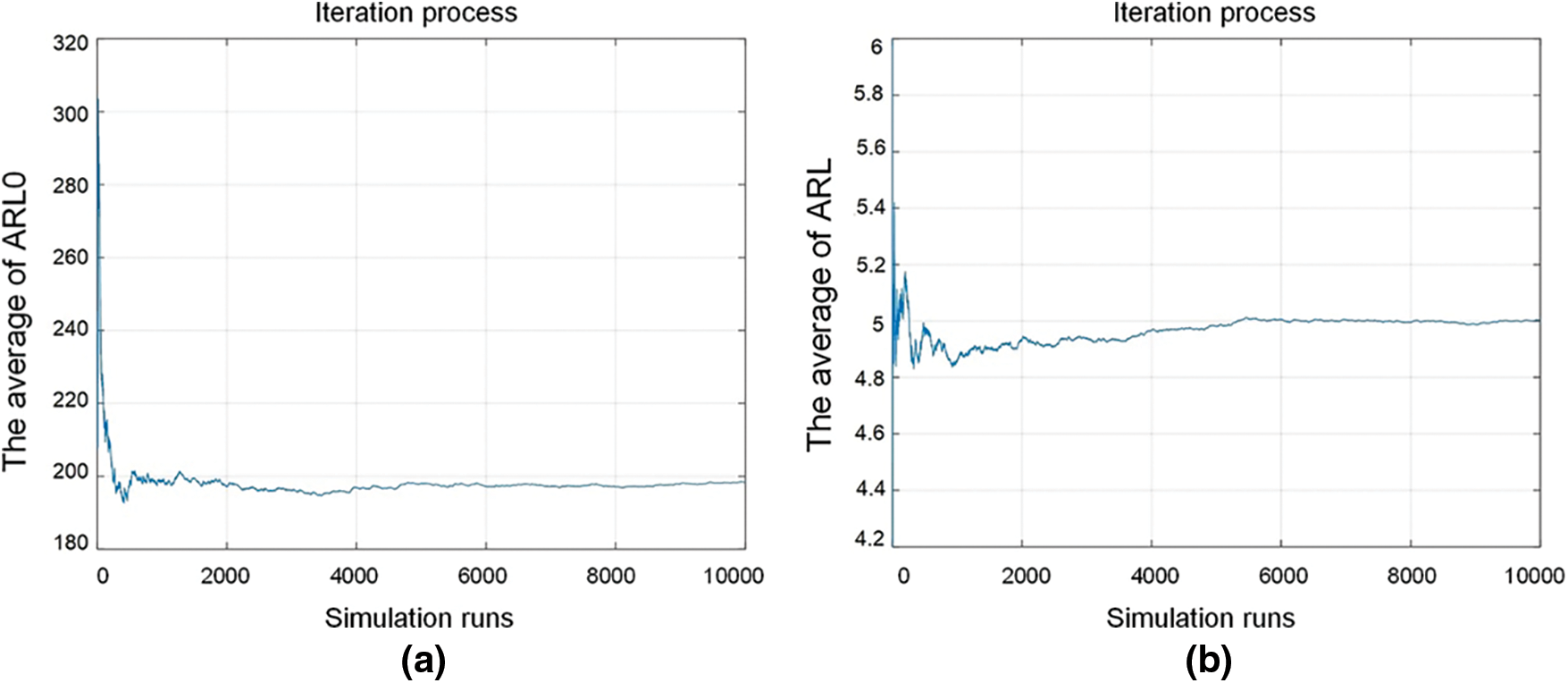
Figure 6: The change of average ARL with simulation runs in the proposed model

The ARLs and SRLs for all abnormal patterns are obtained by the evaluation method introduced in Section 3.3 and presented in Tab. 6. For the convenience of comparison, the minimum ARL values for all levels of mean shift magnitude are highlighted with black border and grey shading in this table. And the minimum SRL values are also highlighted in bold. As shown in Tab. 6, the proposed RF-based model obtains the largest number of minimum ARL values (7 of 15), while BPNN model come in second (6 of 15) and PNN model get the third place (2 of 15). That means the proposed RF model is relatively sensitive to process fluctuations in the bivariate autocorrelated process.

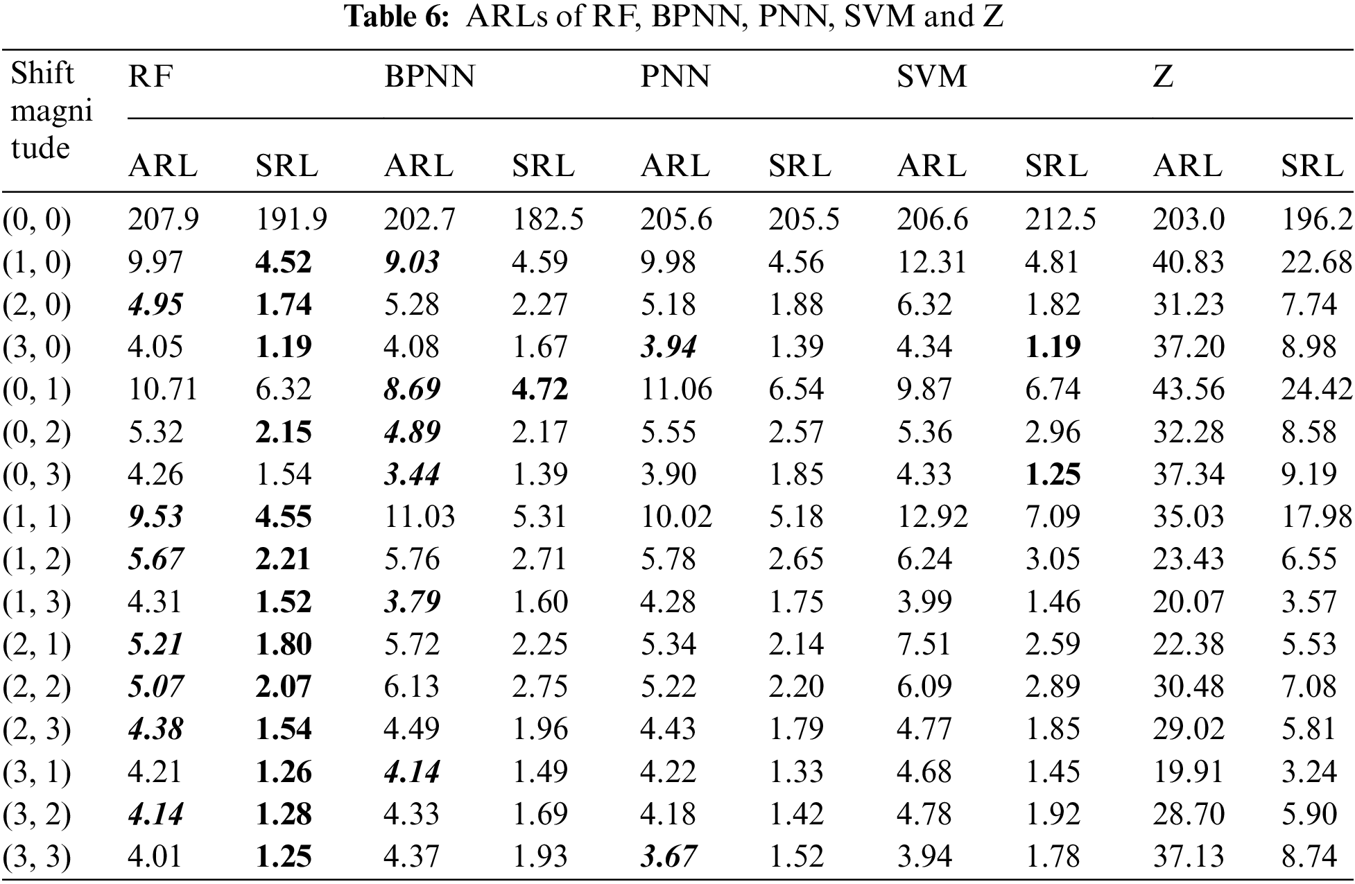
In view of the fact presented by Tab. 6 that the other three models perform much worse than the RF model and the BPNN model, the latter two are further compared here. At first glance, the performance of BPNN model is very close to that of the RF model in terms of ARL. However, as far as the SRL is considered, the RF model performs far better than the BPNN model for it almost produce all the minimum SRL values (13 of 15). As a matter of fact, SRL reflects the stability of detector so is as important as ARL for on-line recognition performance evaluation and should never be ignored. Hence, we think that the proposed RF model is a promising alternative approach for on-line recognition of abnormal patterns in bivariate autocorrelated processes.

5  Conclusion and Future Work

While few cases could be found concerning the autocorrelated multivariate process, it is not uncommon that autocorrelated multivariate process are needed to be monitored in production process. Traditional approaches based on statistics could not meet this need enough. This study proposed a model based on RF to on-line monitor the bivariate autocorrelated process. Data sets of a bivariate autocorrelated process are first established with Monte-Carlo simulation method for training and testing of this model. In order for evaluating this model, a series of comparison experiments are conducted. As the recognition accuracy experiment result show, the model is superior on RA (97.96%) than BPNN (95.69%), PNN (94.31%), and SVM (97.16%). Next, the dynamic experiment result demonstrated that the RF model achieve better ARL and SRL than the other four approaches in most cases of mean shift magnitude. That means the RF model is more promising for on-line monitoring out-of-control signals in the autocorrelated multivariate process, considering that a quicker response for out-of-control situations can better help practitioners to identify the assignable causes and take proper measures rapidly.

Improvements for this model can be made in several ways. For instance, to make this model further identify the abnormal patterns after detecting, or to expand the abnormal pattern from shift to some other typical patterns (e.g., trend and cycle) in the multivariate autocorrelated process. That will be our future work.

Acknowledgement: We are grateful to the editors and all anonymous referees for helpful comments. Additionally, we thank our friends for their contributions to this paper.

Funding Statement: This research was financially supported by the National Natural Science Foundation of China (52065033).

Conflicts of Interest: The authors declare that they have no conflicts of interest to report regarding the present study.

References

 1.  H. Hotelling, Multivariate quality control-illustrated by the air testing of sample bombsights. In: Techniques of Statistical Analysis. New York, USA: McGraw-Hill, pp. 111–184, 1947. [Google Scholar]

 2.  R. B. Crosier, “Multivariate generalizations of cumulative sum quality-control schemes,” Technometrics, vol. 30, no. 3, pp. 291–303, 1988. [Google Scholar]

 3.  C. A. Lowry, W. H. Woodall, C. W. Champ and S. E. Rigdon, “A multivariate exponentially weighted moving average control chart,” Technometrics, vol. 34, no. 1, pp. 46–53, 1992. [Google Scholar]

 4.  S. Bersimis, S. Psarakis and J. Panaretos, “Multivariate statistical process control charts: An overview,” Quality & Reliability Engineering International, vol. 23, no. 5, pp. 517–543, 2007. [Google Scholar]

 5.  H. Alshraideh and E. Khatatbeh, “A gaussian process control chart for monitoring autocorrelated process data,” Journal of Quality Technology, vol. 46, no. 4, pp. 317–322, 2015. [Google Scholar]

 6.  A. V. Vasilopoulos and A. P. Stamboulis, “Modification of control chart limits in the presence of data correlation,” Journal of Quality Technology, vol. 10, no. 1, pp. 20–30, 1978. [Google Scholar]

 7.  N. F. Zhang, “A statistical control chart for stationary process data,” Technometrics, vol. 40, no. 1, pp. 24–38, 1998. [Google Scholar]

 8.  L. C. Alwan and D. Radson, “Time-series modeling for statistical process control,” Journal of Business & Economic Statistics, vol. 6, no. 1, pp. 87–95, 1998. [Google Scholar]

 9.  J. E. Jarrett and X. Pan, “The quality control chart for monitoring multivariate autocorrelated processes,” Computational Statistics & Data Analysis, vol. 51, no. 8, pp. 3862–3870, 2007. [Google Scholar]

10. A. A. Kalgonda and S. R. Kulkarni, “Multivariate quality control chart for autocorrelated processes,” Journal of Applied Statistics, vol. 31, no. 3, pp. 317–327, 2004. [Google Scholar]

11. S. K. Gauri and S. Chakraborty, “Improved recognition of control chart patterns using artificial neural networks,” International Journal of Advanced Manufacturing Technology, vol. 36, no. 11, pp. 1191–1201, 2008. [Google Scholar]

12. A. Ebrahimzadeh and V. Ranaee, “Control chart pattern recognition using an optimized neural network and efficient features,” ISA Transactions, vol. 49, no. 3, pp. 387–393, 2010. [Google Scholar]

13. A. Ebrahimzadeh, J. Addeh and Z. Rahmani, “Control chart pattern recognition using k-mica clustering and neural networks,” ISA Transactions, vol. 51, no. 1, pp. 111–119, 2012. [Google Scholar]

14. A. Addeh, A. Khormali and N. A. Golilarz, “Control chart pattern recognition using RBF neural network with new training algorithm and practical features,” ISA Transactions, vol. 79, no. 19, pp. 202–216, 2018. [Google Scholar]

15. A. Alaeddini and I. Dogan, “Using bayesian networks for root cause analysis in statistical process control,” Expert Systems with Applications, vol. 38, no. 9, pp. 11230–11243, 2011. [Google Scholar]

16. R. S. Guh and Y. R. Shiue, “An effective application of decision tree learning for on-line detection of mean shifts in multivariate control charts,” Computers & Industrial Engineering, vol. 55, no. 2, pp. 475–493, 2008. [Google Scholar]

17. M. Gülbay, C. Kahraman, M. Gülbay and C. Kahraman, Design of fuzzy process control charts for linguistic and imprecise data. In: Fuzzy Applications in Industrial Engineering. Vol. 201. Berlin Heidelberg, GER: Springer, pp. 59–88, 2006. [Google Scholar]

18. K. Demirli and Sr. Vijayakumar, “Fuzzy logic based assignable cause diagnosis using control chart patterns,” Information Sciences, vol. 180, no. 17, pp. 3258–3272, 2010. [Google Scholar]

19. V. Ranaee, A. Ebrahimzadeh and R. Ghaderi, “Application of the pso-svm model for recognition of control chart patterns,” ISA Transactions, vol. 49, no. 4, pp. 577–586, 2010. [Google Scholar]

20. V. Ranaee and A. Ebrahimzadeh, “Control chart pattern recognition using a novel hybrid intelligent method,” Applied Soft Computing Journal, vol. 11, no. 2, pp. 2676–2686, 2011. [Google Scholar]

21. A. Ebrahimzadeh, J. Addeh and V. Ranaee, “Recognition of control chart patterns using an intelligent technique,” Applied Soft Computing, vol. 13, no. 5, pp. 2970–2980, 2013. [Google Scholar]

22. S. Du, D. Huang and J. Lv, “Recognition of concurrent control chart patterns using wavelet transform decomposition and multiclass support vector machines,” Computers & Industrial Engineering, vol. 66, no. 4, pp. 683–695, 2013. [Google Scholar]

23. X. Petros and R. Talayeh, “A weighted support vector machine method for control chart pattern recognition,” Computers & Industrial Engineering, vol. 70, no. 1, pp. 134–149, 2014. [Google Scholar]

24. A. Khormali and J. Addeh, “A novel approach for recognition of control chart patterns: type-2 fuzzy clustering optimized support vector machine,” Isa Transactions, vol. 63, no. 1, pp. 256–264, 2016. [Google Scholar]

25. H. S. Zhang, B. Zhu, K. M. Pang, C. M. Chen and Y. W. Wan, “Identification of abnormal patterns in ar (1) process using cs-svm,” Intelligent Automation & Soft Computing, vol. 28, no. 3, pp. 797–810, 2021. [Google Scholar]

26. H. B. Hwarng and Y. Wang, “Shift detection and source identification in multivariate autocorrelated processes,” International Journal of Production Research, vol. 48, no. 3, pp. 835–859, 2010. [Google Scholar]

27. A. Fountoulaki, N. Karacapilidis and M. Manatakis, “Using neural networks for mean shift identification and magnitude of bivariate autocorrelated processes,” International Journal of Quality Engineering & Technology, vol. 2, no. 2, pp. 114–128, 2011. [Google Scholar]

28. C. Zhang and Z. He, “Mean shifts identification in multivariate autocorrelated processes based on PSO-SVM pattern recognizer,” in Proc. of 2012 3rd Int. Asia Conf. on Industrial Engineering and Management Innovation (IEMI2012), Berlin Heidelberg, Springer, pp. 225–232, 2013. [Google Scholar]

29. L. Breiman, “Random forests,” Machine Learning, vol. 45, no. 1, pp. 5–32, 2001. [Google Scholar]

30. A. Assiri, “Anomaly classification using genetic algorithm-based random forest model for network attack detection,” Computers Materials & Continua, vol. 66, no. 1, pp. 767–778, 2021. [Google Scholar]

31. Z. Yu, C. Zhang, N. Xiong and F. Chen, “A new random forest applied to heavy metal risk assessment,” Computer Systems Science and Engineering, vol. 40, no. 1, pp. 207–221, 2022. [Google Scholar]

32. C. J. Su, X. Y. Li, M. R. Li, Q. S. Zhu, H. Fu et al., “Improved prediction and understanding of Glass-forming Ability Based on Random Forest Algorithm,” Journal of Quantum Computing, vol. 3, no. 2, pp. 79–87, 2021. [Google Scholar]

33. M. Li, Z. Fang, W. Cao, Y. Ma, S. Wu et al., “Residential electricity classification method based on cloud computing platform and random forest,” Computer Systems Science and Engineering, vol. 38, no. 1, pp. 39–46, 2021. [Google Scholar]

34. B. Zhu, B. B. Liu, Y. W. Wan and S. R. Zhao, “Recognition of control chart patterns in auto-correlated process based on Random Forest,” in Proc.-2018 IEEE Int. Conf. on Smart Manufacturing, Industrial and Logistics Engineering (SMILE), Hsinchu, Taiwan, China, pp. 53–57, 2018. [Google Scholar]

35. Y. W. Wan and B. Zhu, “Abnormal patterns recognition in bivariate autocorrelated process using optimized random forest and multi-feature extraction,” ISA Transactions, vol. 109, no. 4, pp. 102–112, 2021. [Google Scholar]

This work is licensed under a Creative Commons Attribution 4.0 International License, which permits unrestricted use, distribution, and reproduction in any medium, provided the original work is properly cited.