Computers, Materials & Continua DOI:10.32604/cmc.2022.027776
Article

Resource Load Prediction of Internet of Vehicles Mobile Cloud Computing

Wenbin Bi1, Fang Yu2, Ning Cao3,* and Russell Higgs4

1School of Computer and Software, Dalian Neusoft University of Information, Dalian, 116023, China
2School of Information Engineering, Qingdao Bin Hai University, Qingdao, China
3School of Internet of Things and Software Technology, Wuxi Vocational College of Science and Technology, Wuxi, 214028, China
4School of Mathematics and Statistics, University College Dublin, Dublin, Ireland
*Corresponding Author: Ning Cao. Email: ning.cao2008@hotmail.com
Received: 25 January 2022; Accepted: 23 March 2022

Abstract: Load-time series data in mobile cloud computing of Internet of Vehicles (IoV) usually have linear and nonlinear composite characteristics. In order to accurately describe the dynamic change trend of such loads, this study designs a load prediction method by using the resource scheduling model for mobile cloud computing of IoV. Firstly, a chaotic analysis algorithm is implemented to process the load-time series, while some learning samples of load prediction are constructed. Secondly, a support vector machine (SVM) is used to establish a load prediction model, and an improved artificial bee colony (IABC) function is designed to enhance the learning ability of the SVM. Finally, a CloudSim simulation platform is created to select the per-minute CPU load history data in the mobile cloud computing system, which is composed of 50 vehicles as the data set; and a comparison experiment is conducted by using a grey model, a back propagation neural network, a radial basis function (RBF) neural network and a RBF kernel function of SVM. As shown in the experimental results, the prediction accuracy of the method proposed in this study is significantly higher than other models, with a significantly reduced real-time prediction error for resource loading in mobile cloud environments. Compared with single-prediction models, the prediction method proposed can build up multidimensional time series in capturing complex load time series, fit and describe the load change trends, approximate the load time variability more precisely, and deliver strong generalization ability to load prediction models for mobile cloud computing resources.

Keywords: Internet of Vehicles mobile cloud computing; resource load predicting; multi distributed resource computing scheduling; chaos analysis algorithm; improved artificial bee colony function

1  Introduction

In the IoV, smart vehicles have to collect, process and transmit a so huge scale of information in real time that it is very difficult to completely rely on the vehicles themselves to meet all data requirements. In addition, people’s needs for multimedia on their trips are increasing day by day. As a result, such services as music and videos are also taking up a large amount of communication, computing and storage resources of vehicles, while putting forward higher requirements on real-time performance. However, mobile cloud computing technology has brought effective solutions to the IoV. With the development of the IoV business, an increasingly massive number of operations are required, leading to heavy computing workloads. IoV clouds combined with mobile cloud computing will become an effective approach to solving such problems [1,2]. As a mobile cloud computing paradigm, the vehicle cloud network regards the on-board terminal mounted in a vehicle on road as a resource unit and integrates the computing and storage capabilities on the vehicle side, in combination with vehicle-to-vehicle communication (V2V). The vehicle cloud network based on mobile cloud computing can effectively utilize vehicle resources to provide low-latency cloud services, while improving the dynamic accessibility of resources [3]. However, due to the limited scope and scale of the vehicle cloud network, how to efficiently manage and allocate resources becomes a major problem with such networks. There are three types of IoV resources: communication resources, computing resources and storage resources [4].

Resource load prediction of IoV mobile cloud computing is the basis of resource scheduling [5–7]. Most resource load models of IoV mobile cloud computing rely on time series data [8–10]. Generally [11], they regard the IoV mobile cloud computing resource loads at different times as a time series, and then fit the relationships between the IoV mobile cloud computing resource load-time series data by using certain modeling methods, so as to find out the changing characteristics of IoV mobile cloud computing resource load and predict the future trends of such loads [12,13]. At present, the modeling methods in this respect mainly include neural networks, grey models [14] and so on. However, grey models can only predict the rising or falling trends of resource loads in IoV mobile cloud computing, and such loads are related to many factors, while showcasing strong time-varying characteristics [15]. Nevertheless, the neural network has some defects, such as slow convergence speed, over-fitting and so on [16]. The construction of learning samples for such loads is a key step in the modeling process. At present, the chaos of time series is not well considered in the prediction of such loads, with low prediction accuracy of their change trends [17].

The load-time series data of mobile cloud computing of IoV usually demonstrate the linear and nonlinear composite characteristics, and the existing models cannot accurately describe the dynamic change trends of loads [18]. This study proposes a SVM-based method for mobile cloud computing resource load prediction. Firstly, a chaotic analysis algorithm is used to process the load time series of mobile cloud computing resources, and a learning sample for mobile cloud computing resource load prediction is constructed. Then, SVM is used to build up a load prediction model for mobile cloud computing resources, while an IABC function is designed to improve the learning ability of SVM. Finally, cloud computing resource load prediction experiments are conducted to verify the performance of the proposed method compared with other models.

2  Related Work

2.1 Mobile Cloud Computing Resource Scheduling Model for Internet of Vehicles

In the existing mobile edge computing resource unloading strategies, more consideration is given to the unloading of a single mobile cloud computing resource. Different kinds of computing resources are not considered, which is easy to lead to low energy consumption optimization [19]. According to the actual characteristics of mobile cloud computing resources under the IoV, this study proposes a computing scheduling model based on multi distributed resources. The model includes three cases: the task is not unloaded, the task is unloaded to other vehicles in the vehicle cloud network, and the task is unloaded to the traditional cloud server.

2.1.1 Task Without Unloading

Tedge=∑i=1nlifedge(1)

Tedge is the processing time of the task at the edge of the IoV, li is the task load of i, and fedge is the processing speed of the task at the edge of the IoV.

Eedge=Pedge×Tedge(2)

Eedge is the execution energy consumption and Pedge is the execution power.

2.1.2 Task is Unloaded to Other Vehicles

Eec=Ptr×CjR1+Pre×djR2+Pidle×Tec(3)

Eec is the energy consumption level during the unloading of task Ti to other vehicles in the vehicle cloud network, Ptr is the transmission data power, Pre is the reception data power, Pidle is the idle power, R1 and R2 are the data transmission rate and reception rate, Cj and Dj are the transmission size and reception size of task data respectively, and Tec is the task execution time.

Tec=∑j=1nljfec(4)

lj is the task load of j and fec is the running speed of other vehicles.

2.1.3 Task is Uniloaded to Traditional Cloud Server

Ecc=Ptr×CkR1+Pre×dkR2+Pidle×Tcc(5)

Ck and dk are the data transmission and reception speeds during task execution.

2.2 Fitness Algorithm of Mobile Cloud Computing Resource Scheduling Model for Internet of Vehicles

The execution time and cost of task scheduling were evaluated by fitness. The greater the fitness, the higher the energy consumption of the scheduling scheme. On the contrary, the smaller the fitness, the lower the energy consumption [20].

2.2.1 Algorithm Fitness

fitness=(f1×Esum)+(f2×10×Esum×TsumTreponse)(6)

Esum=∑i=1maxEedge+∑j=1maxEec+∑k=1maxEcc(7)

Tsum=∑i=1maxTedge+∑j=1maxTec+∑k=1maxTcc(8)

fitness is the energy consumption fitness, Esum is the total energy consumption, Tsum and Treponse are the total task execution time and task response time. f1 is the response speed and f2 is the execution speed. The algorithm flow chart is shown in Fig. 1 below.

2.2.2 Algorithm Flow

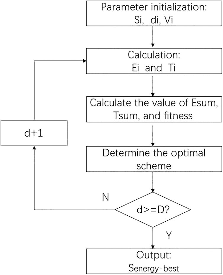
Figure 1: Algorithm flow diagram

The flow chart is described below.

1.    Randomly initialize the task scheduling scheme Si, unloading decision di and search speed Vi.

2.    Calculate the energy consumption and execution time of the scheduling scheme Si unloaded to the three resources.

3.    Calculate the total energy consumption, total execution time and fitness value of the scheduling scheme.

4.    The optimal scheduling scheme is selected according to the fitness value, and the scheme with the lowest fitness is regarded as the global optimal scheduling scheme.

5.    Update the scheduling scheme according to the search speed and provide the unloading decision of each task. Update the search speed of the scheduling scheme according to the inertia weight strategy. When the set number of iterations D is reached, the energy consumption optimal scheduling scheme Senergy-best under the response time constraint is obtained.

6.    Calculate the energy consumption and time of unloading the scheduling scheme Si to three resources.

7.    Calculate the total energy consumption, time and fitness of the dispatching scheme.

8.    The scheme with the lowest fitness value is selected as the global optimal scheme.

9.    Update the search speed of the scheduling scheme. When the set number of iterations D is reached, the energy consumption optimization scheduling scheme Senergy-best is output.

2.3 Artificial Bee Colony Algorithm (ABC Algorithm )

Artificial bee colony (ABC) algorithm consists of food sources, employed bees and unemployed bees. The bees were divided into three groups: employed bees, onlookers and scouts. Employed bees and unemployed bees accounted for half of the total number of bees, and the path planning process was divided into search process and optimization process [21].

2.3.1 Search Process

Food point xi(i∈1,2,⋯,SN) represents a viable solution. All positions xi(i∈1,2,⋯,SN) have parameters D(xij,j∈1,2,⋯,D) to be optimized. Food point initialization is defined as follows.

xij=lj+rand(0,1)(uj−lj)(9)

In the equation, lj and uj are the lower and upper limits of parameter j, rand (0,1) is the uniform random number between 0 and 1, and Sn is the number of food sources.

2.3.2 Optimization Process

(1) Employed bees stage: Each employed bee corresponds to the food location. The employed bees conduct a local search near their current food location to find a new food location. The calculation equation is:

vij=xij+ϑij(xij−xkj)(10)

(2) Onlookers stage: After the employed bees deliver the honey to the hive, they invite the onlookers to fly with them to the food source. Whether the onlookers accept the invitation is mainly related to the quality of food source that the employed bees depend on. The onlookers determined the selection probability of food source by roulette according to Eq. (11) according to the income degree of food source.

pi=fiti∑i=1SNfiti(11)

In Eq. (11), pi is the probability of scouts to choose food source, and fiti is the income degree of food source. Once the onlookers have selected a food location, they generate a new food location using Eq. (10), evaluate the new food location and apply the same greedy choice.

(3) Scouts stage: A more optimized solution in the solution space is sought by enlarging the search area. If the food location is not improved after repeated experiments, the leading bees will become scouts and randomly generate new food spots through Eq. (9), and then search for new food sources according to Eq. (11).

(4) Optimal food source determination stage: After the above several stages, the optimal food source is obtained by judging whether the termination condition is satisfied. The employed bees and scouts are used for local and global search respectively, while the onlookers are used for the balance between them. Finally, the optimal solution is found through multiple iterations and cyclic updates in three stages.

2.4 Improved Artificial Bee Colony (IABC Algorithm)

The adjustment of trigonometric function is introduced into Eq. (10), which makes ABC algorithm perform better in both local search and global search. At the same time, in order to improve the search accuracy, the new bee individual takes itself as the origin and searches within the maximum radius from itself to the optimal bee of this subgroup.

vij=xijsin⁡(tπ2G)+ϑij(xij−xkj)cos⁡(tπ2G)rmax(12)

In Eq. (12): t=1,2,⋯,G, G is the fixed number of evolutionary iterations, and rmax is the maximum radius of the field of the bee individual with the best global fitness.

It can be seen from Eq. (11) that the greater the income of food source, the greater the probability of being selected by onlookers, and the more onlookers around it. However, with the increase of calculation times, the population diversity will decrease. To solve this problem, when determining the probability of food source selection, N onlookers chose food source by roulette, and N onlookers chose food source by Eq. (13), so that the food source with lower income could also be selected and the diversity of the population could be increased.

pi=exp⁡(−1δ×fiti)(13)

In Eq. (13), δ is the parameter in the improved algorithm. It can be seen that the probability value of food source being selected is inversely proportional to the income degree, and it decreases with the increase of the income degree.

ABC algorithm, like other evolutionary algorithms, has the defect of falling into local optimal solution prematurely, but it can jump out of local optimal solution by increasing population diversity. In the onlooker stage, the reverse evolution operator as shown in Eq. (13) is added to make the population evolve in two directions. The existence of roulette ensures that the food source with the best income in each generation is retained. The existence of Eq. (13) preserves food sources with low income, ensures the diversity of population, improves the global search ability and convergence speed of the algorithm, and can better solve the problem of dynamic target allocation.

2.5 Cross-Correlation(C-C) Algorithm

C(m,N,r,t)=2m(m−1)∑1≤i≤j≤Nθ(r−‖Xi−Xj‖(∞))(14)

In Eq. (14): m is the embedding dimension, N is the number of samples in the time series, r is the radius of the time series, and t is the number of subsequences. Xi is the i-th subsequence, Xj is the j-th subsequence, ‖Xi − Xj‖ (∞) is an infinite norm, and θ(x)={0x≤01x>0.

Define the test statistic of the sequence x={xi} as:

S(m,N,r,t)=C(m,N,r,t)−Cm(m,N,r,t)(15)

The time series x={xi|i=1,2,⋯,N} is divided to get t subseries, then the following equation is obtained:

{x(1)={x1,xt+1,⋯,x⌊N/t⌋−t+1}x(2)={x2,xt+2,⋯,x⌊N/t⌋−t+2}⋮x(t)={xt,xt+t,⋯,x⌊N/t⌋}(16)

The block average strategy is adopted to calculate the statistics of Eq. (16), as follows:

S1(m,N,r,t)=1t∑s=1t[Cs(m,N,r,t)−Csm(1,N,r,t)](17)

In Eq. (17), r represents the distance between any two points. If N goes to infinity, we get the following equation.

S1(m,r,t)=1t∑s=1t[Cs(m,r,t)−Csm(1,r,t)](18)

When the length of time series is infinite, S(m,r,t)=0. However, in practical application, the length of time series is limited, so S(m,r,t)≠0. The local maximum time interval method is adopted to select the time point with the smallest difference in radius r, then the following equation can be obtained.

ΔS1(m,t)=max{S1(m,rj,t,N)}−min{S1(m,rj,t,N)}(19)

In Eq. (19) rj represents the value of the j-th radius. According to Eq. (19), the optimal t′ is the first local minimum of ΔS1(m,t)∼t, according to Brock Dechert Scheinkman’s statistical conclusion, the following equation is obtained.

S¯1(t)=116∑m=14∑m=14S1(m,r,t)(20)

ΔS¯1(t)=14∑m=14ΔS1(m,t)(21)

Define S1cor(r)=ΔS¯1(t)+|S¯1(t)|, then S1cor(r) reaches the minimum value, the optimal embedding window can be obtained, and the optimal embedding dimension m can be obtained according to Eq. (22).

tw′=(m−1)t′(22)

3  Resource Load Forecasting Framework of IoV Mobile Cloud Computing Based on C-C and IABC

3.1 Resource Load Forecasting Framework for Internet of Vehicles Mobile Cloud Computing

The processing flow of this framework is shown below.

1.    Collect time series data of resource load of 1 Internet of vehicles mobile cloud computing.

2.    The C-C method is used to determine the optimal m and t of the time series of the mobile cloud computing resource load of the IoV.

3.    Build a multi-dimensional time series according to the optimal m and t, which is the learning sample of resource load prediction modeling of IoV mobile cloud computing.

4.    The training samples of the resource load of IoV mobile cloud computing are used for learning, and the resource load prediction model of IoV mobile cloud computing is established. For one example, see Fig. 2 below.

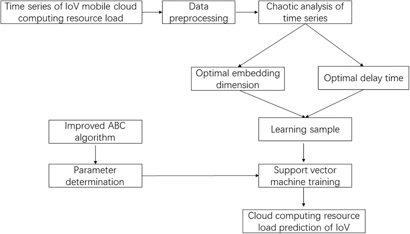
Figure 2: Resource load forecasting framework of IoV mobile cloud computing based on C-C and IABC

3.2 Load Forecasting Method under Mobile Cloud Computing Resource Scheduling Model of Internet of Vehicles

The load prediction process under the resource scheduling model of mobile cloud computing in the IoV refers to the genetic algorithm and is divided into two stages. The inner layer is the forecasting stage and the outer layer is the scheduling stage. The fitness function of the inner layer is the energy consumption cost of each resource. After the initial population is generated, the energy consumption allocation of the next generation of resources is generated. Each generation produces a new population through excellent individual selection, individual crossover and variation. The population evolves until it reaches the termination condition of the number of iterations. The goal of the whole process is to find the resource allocation that optimizes the energy consumption cost under the corresponding task resource allocation condition. The fitness function of the outer layer is the global relaxation time under each task resource allocation. After the initial population is generated, the next generation task resource allocation is generated. Each generation also produces new populations through excellent individual selection, individual crossover and variation. The population evolves until it reaches the termination condition of the number of iterations. The goal of the whole process is to find the computational cost under the task resource allocation and the corresponding optimal allocation of resource energy consumption. For one example, see Fig. 3 below.

4  Experiment on Resource Load Prediction Framework of IoV Mobile Cloud Computing Based on C-C and IABC

4.1 Performance Experiment of IoV Mobile Cloud Computing Resource Load Prediction Framework

4.1.1 Experimental Data

In order to test the performance of the resource load prediction model of IoV mobile cloud computing proposed in this study, the simulation of virtual resource scheduling is carried out by using CloudSim simulation platform. We increase the usage of CPU, memory and network bandwidth by using a surge in traffic. We chose the CPU load history data per minute in a mobile cloud computing system consisting of 50 vehicles as the research object. At present, there are two methods to judge and analyze the chaos of time series: quantitative analysis and qualitative analysis. In this study, the Lyapunov exponent method in qualitative analysis is used to analyze the chaotic characteristics of mobile cloud computing resource load data. The specific steps are as follows:

(1) Fourier transform is used to process the mobile cloud computing resource load data, and calculate the average track period T of the mobile cloud computing resource load data of the Internet of vehicles.

(2) The C-C method is used to determine the optimal m and T of the IoV mobile cloud computing resource load data, and the reconstructed multi-dimensional time series y of the IoV mobile cloud computing resource load is obtained Yj, j = 1,2,⋯,M.

(3) Calculate the distance between the i-th discrete time of each point Yj and the adjacent point.

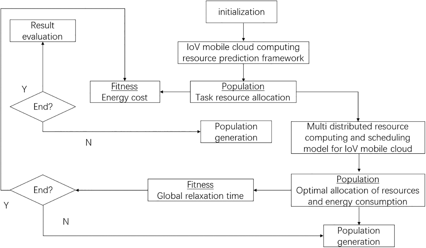
Figure 3: Load forecasting process under the resource scheduling model of IoV mobile cloud computing

dj(i)=‖Yj+1−Yj+i‖i=1,2,⋯,min(M−j,m−i)(23)

(4) Calculate the average of all dj(i).

y(i)=1qΔt∑j=1qln⁡dj(i)(24)

q represents the number of ln⁡dj(i)≠0.

According to the above steps, the Lyapunov exponent is 0.0995 > 0, which indicates that the historical data of the resource load of mobile cloud computing in the Internet of vehicles has chaotic performance. According to the C-C method, the best t = 7 and the best tw = 12 of the historical data of the resource load of the IoV mobile cloud computing are determined, and then the best embedding dimension m = 3 is obtained according to tw and t. t = 7 and m = 3 are used to construct the load learning sample of IoV mobile cloud computing resources.

4.1.2 Results and Analysis

(1) Single step prediction results of the resource load prediction model for IoV mobile cloud computing

Select the last 100 data points in the network of vehicles mobile cloud computing resource load as the test samples, and other data points as the training samples of the network of vehicles mobile cloud computing resource load prediction model for learning, build the network of vehicles mobile cloud computing resource load prediction model, and conduct one-step prediction on the test samples to obtain the one-step prediction results of the network of vehicles mobile cloud computing resource load, see Fig. 4 below.

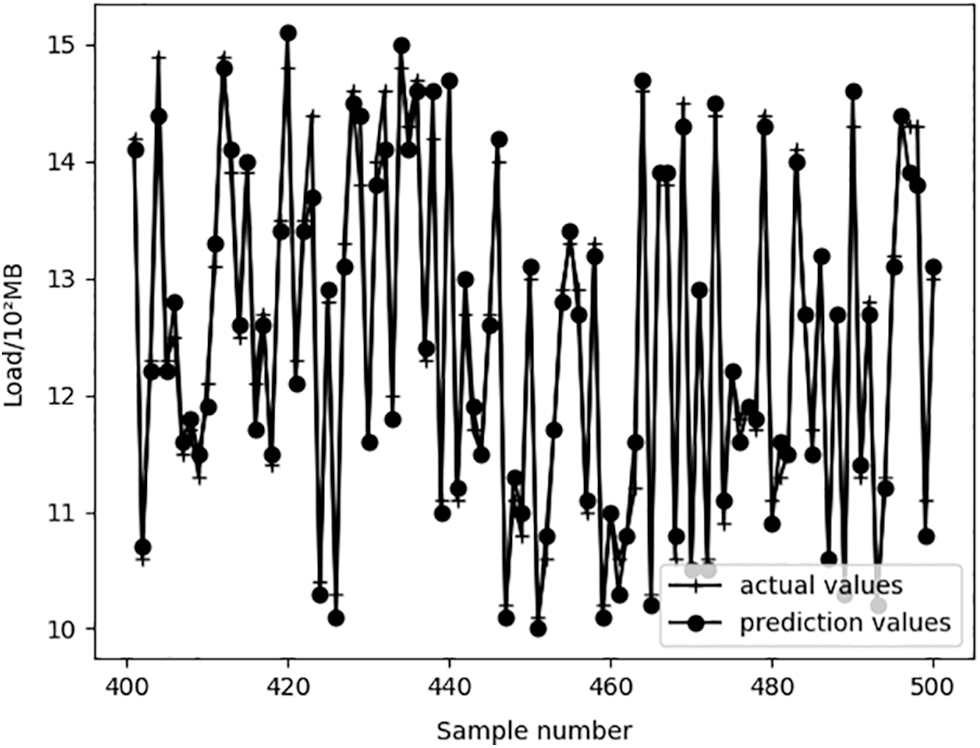
Figure 4: Single step prediction results

Through the analysis of the resource load prediction results of IoV mobile cloud computing, it can be found that the addition of support vector machine method can effectively track the change trend of IoV mobile cloud computing resource load, and obtain high-precision IoV mobile cloud computing resource load prediction results.

(2) Multi step prediction results of resource load prediction model for IoV mobile cloudcomputing

The prediction of the resource load of the mobile cloud computing of the IoV is mainly to analyze the change trend of the resource load of the mobile cloud computing of the IoV in the future. The single-step prediction results can only describe the resource load of the mobile cloud computing of the IoV in the next moment. Therefore, it is necessary to carry out the multi-step prediction of the resource load of the mobile cloud computing of the IoV. The resource load prediction results of IoV mobile cloud computing three steps in advance are shown in Fig. 5.

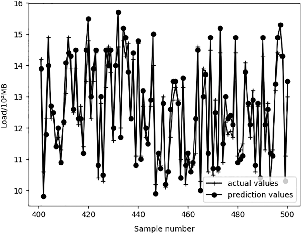
Figure 5: Multi step prediction results

As can be seen from Fig. 5, the multi-step resource load prediction results of Internet of vehicles mobile cloud computing are significantly worse than the single-step resource load prediction results of IoV mobile cloud computing. However, this model can still better describe the change trend of IoV mobile cloud computing resource load. The prediction results have a certain reference value for IoV mobile cloud computing resource load management.

(3) Comparative experiment on resource load prediction performance of IoV mobile cloud computing with other models.

In order to test the superiority of the method in this study, the grey model, back propagation (BP) neural network, radial basis function (RBF) neural network and SVM with RBF kernel function are selected for the comparative experiment of resource load prediction of mobile cloud computing in vehicle networking, The load prediction accuracy of IoV mobile cloud computing resources is counted, and the results are shown in Fig. 6.

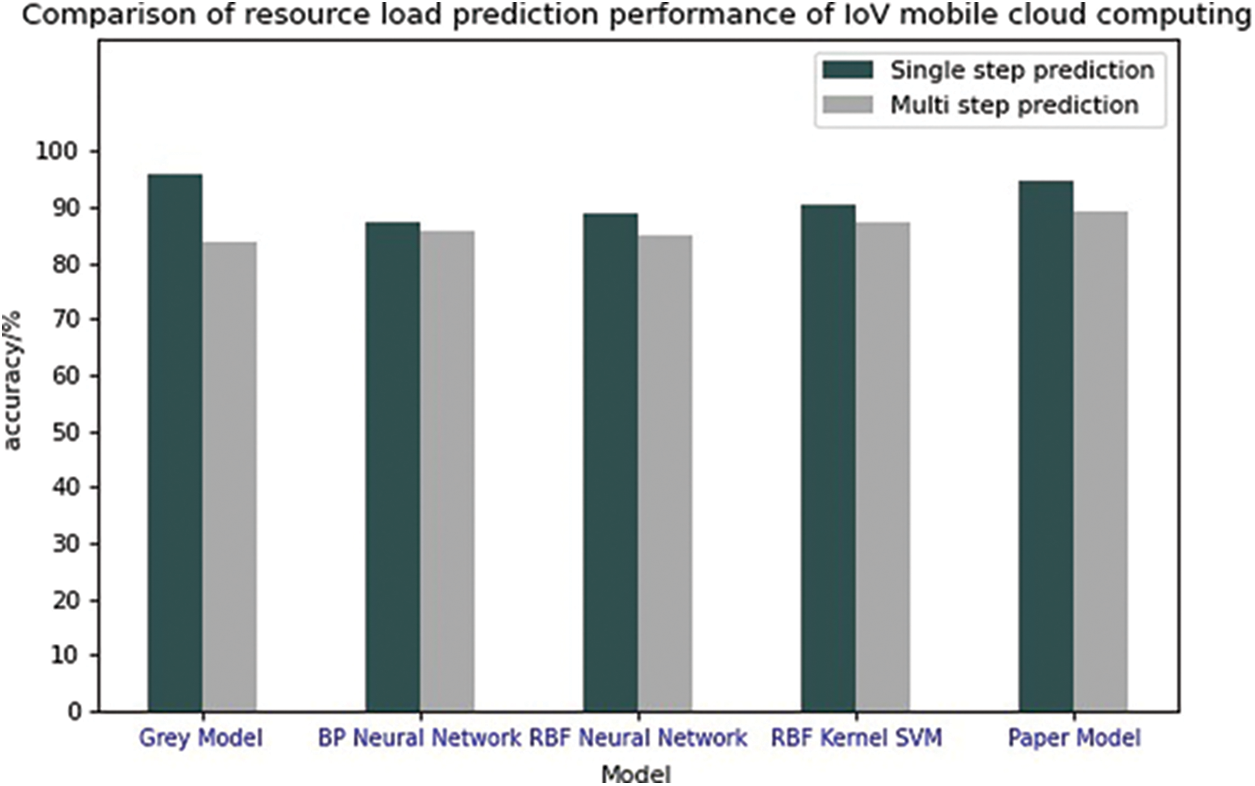
Figure 6: Comparison of resource load prediction performance of IoV mobile cloud computing

By comparing and analyzing the load prediction accuracy of IoV mobile cloud computing resources in Tab.1, it is found that when multi-step IoV mobile cloud computing resource load prediction is carried out, the prediction accuracy of this model is the highest, which better overcomes the defects of other IoV mobile cloud computing resource load prediction models.

4.2 Experiment of Load Forecasting Method Under the Resource Scheduling Model of Mobile Cloud Computing in the IoV

4.2.1 Evaluation Criterion

Considering the linear and nonlinear characteristics of load time series data, this paper proposes an error correction combined prediction model, which better reflects the change trend of load time series with time. The prediction results were evaluated by mean absolute error (MAE), mean absolute value percentage error (MAPE), mean squared error (MSE), root mean squared error (RMSE), and R-squared (R2).

MAE=1n∑i=1n|yi−y^i|(25)

MAPE=1n∑i=1n|yi−y^iyi|(26)

MSE=1n∑i=1n(yi−y^i)2(27)

RMSE=1n∑i=1n(yi−y^i)2(28)

R2=1−∑i=1n(yi−y^i)2∑i=1n(yi−y¯)2(29)

n is the number of load prediction values, yi is the actual load value, y^i is the predicted load value, y¯ is the average load.

4.2.2 Experimental Results and Analysis

In order to verify the effectiveness of the proposed load forecasting model of Internet of vehicles mobile cloud computing resources, the above simulation data are used to verify the load forecasting method under the Internet of vehicles mobile cloud computing resource scheduling model proposed in this paper. In order to test and evaluate the performance of the load forecasting method under the Internet of vehicles mobile cloud computing resource scheduling model proposed in this paper, it is also compared with the single algorithm of ARIMA, BP, SVM [22,23] and LSTM [24–26]. At the same time, it is also compared with the ARIMA-ANN (A-ANN) combined forecasting model proposed in literature [27–29], [30–32]. Use the data of the past hour to predict the data of the next 5 min. Based on experience and comparison with many experiments, the relevant parameters of the single-step load forecasting model are set as follows, see Tab. 1.

The measured workload value of 10 days is selected from the data set. By analyzing the load data, the weights of CPU utilization and memory utilization are set to 0.4 and 0.6 respectively, with a total of 2880 data records. The first 70% of the data are selected as the training set, 20% of the data are selected as the one-step test set, and the remaining data are used to verify the generalization ability of the model, see Fig. 7.

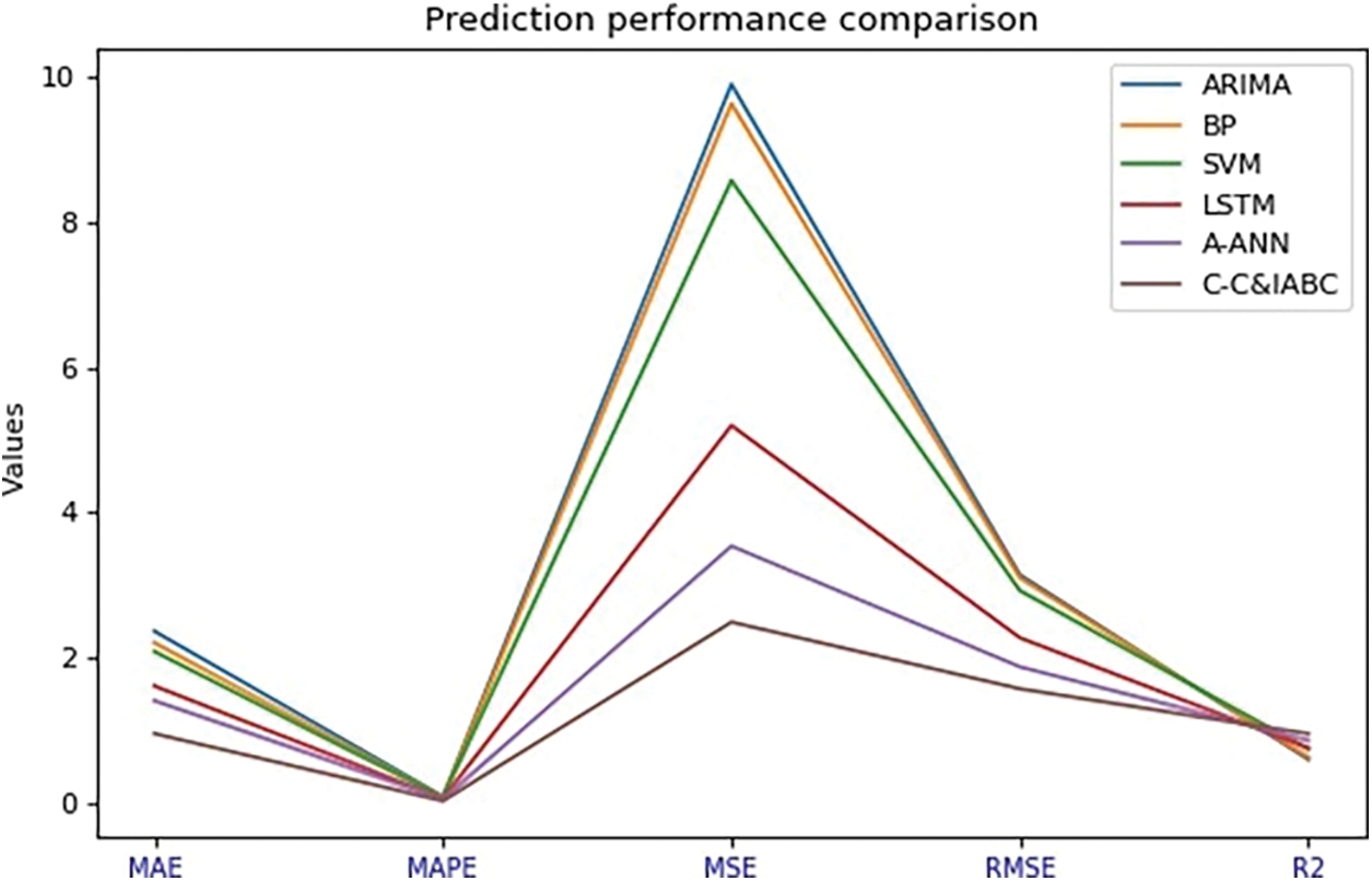
Figure 7: Prediction performance comparison

From the Fig. 7, the trend of all algorithms is basically the same as that of the original sequence, but the prediction accuracy of the single load prediction model is obviously lower than that of the combined prediction model. The load forecasting model proposed in this paper has higher accuracy than the traditional load forecasting model.

The mobile cloud computing resource load prediction of the IoV mainly analyzes the change trend of the mobile cloud computing resource load in the future. The one-step prediction results can only describe the load in the cluster at the next moment. In order to further verify the generalization ability of the proposed model, the original resource load sequence is calculated every 6 points to construct the IoV mobile cloud computing resource load data with an average interval of 30 min. Similarly, the IoV mobile cloud computing load data with an interval of 60 min is constructed. For the prediction results of 30 min and 60 min intervals, the detailed error analysis is shown in Fig. 8.

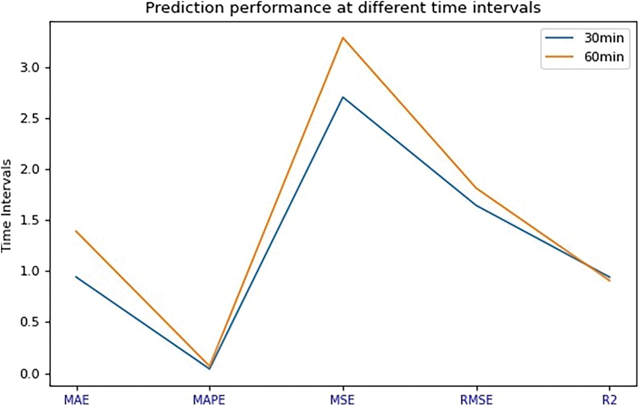
Figure 8: Prediction performance at different time intervals

It can be observed from the prediction results that the method proposed in this study can accurately predict the load value of mobile cloud computing resources in the IoV in different time intervals. Although the prediction result of multi-step mobile cloud computing resource loads is outperformed by that of single-step mobile cloud computing resource loads, with increasingly more load samples, the original time series is analyzed and reconstructed to create a multi-dimensional time series, which can better reflect the load change characteristics of mobile cloud computing resources. The IABC function is introduced to construct a support vector machine, which can overcome the disadvantages of the existing support vector machines, extract the hidden features of the whole sequence, refine the approximation of the load time-variability of mobile cloud computing resources, and deliver a stronger generalization ability for the new load prediction model.

5  Conclusions and Future Work

Aiming at addressing the chaos of complex and changeable load sequences of mobile cloud computing of IoV, while considering the influence of energy consumption optimization, this study proposes a SVM-based load prediction method for mobile cloud computing resources of IoV under multi-distributed resource computing scheduling. In this method, the chaos theory is introduced to analyze and reconstruct the original time series, and a multi-dimensional time series is also created to better showcase the load change characteristics of mobile cloud computing resources in the IoV. Since the SVM has good generalization abilities, an IABC function is introduced to build up the SVM, which can approach the load time variability of mobile cloud computing resources in the IoV in a more precise manner. The single- and multi-step prediction simulation results show that the prediction accuracy of the model proposed in this study can reach 94.87%, only lower than the 95.85% accuracy of the grey model. When it comes to prediction of the load of mobile cloud computing resources in the IoV, the prediction accuracy of the model of this study reaches 89.18%, which can effectively track the load variation of such resources. The experimental results show that the proposed method can provide good prediction accuracy, while significantly reducing the real-time prediction error of resource load in the mobile cloud environment of the IoV. In the follow-up research, more consideration shall be given to such constraints as dynamic changes in users’ time and energy weight allocations according to actual individual situations and other disturbances, and more experimental samples shall be used to verify the rationality of the algorithm of this study.

Funding Statement: This work was supported by Shandong medical and health science and technology development plan project (No.202012070393).

Conflicts of Interest: The authors declare that they have no conflicts of interest to report regarding the present study.

References

 1.  J. G. Ibanez, S. Zeadally and J. Contreras-Castillo, “Integration challenges of intelligent transportation systems with connected vehicle, cloud computing, and internet of things technologies,” IEEE Wireless Communications, vol. 22, no. 6, pp. 122–128, 2015. [Google Scholar]

 2.  M. Sookhak, F. R. Yu and H. Ying, “Fog vehicular computing: Augmentation of fog computing using vehicular cloud computing,” IEEE Vehicular Technology Magazine, vol. 12, no. 3, pp. 55–64, 2017. [Google Scholar]

 3.  Z. Jiang, S. Zhou and X. Guo, “Task replication for deadline-constrained vehicular cloud computing: Optimal policy, performance analysis and implications on road traffic,” IEEE Internet of Things Journal, vol. 5, no. 1, pp. 93–107, 2018. [Google Scholar]

 4.  R. Yu, X. Huang and J. Kang, “Cooperative resource management in cloud-enabled vehicular networks,” IEEE Transactions on Industrial Electronics, vol. 62, no. 12, pp. 7938–7951, 2015. [Google Scholar]

 5.  B. Osibo, C. Zhang, C. Xia, G. Zhao and Z. Jin, “Security and privacy in 5G internet of vehicles (IoV) environment,” Journal of Internet of Things, vol. 3, no. 2, pp. 77–86, 2021. [Google Scholar]

 6.  D. A. Shafiq, N. Jhanjhi and A. Abdullah, “Machine learning approaches for load balancing in cloud computing services,” in 2021 National Computing Colleges Conf. (NCCC), Taif, Saudi Arabia, pp. 1–8, 2021. [Google Scholar]

 7.  Z. A. Almusaylim and N. Z. Jhanjhi, “Comprehensive review: Privacy protection of user in location-aware services of mobile cloud computing,” Wireless Personal Communications, vol. 111, no. 1, pp. 541–564, 2020. [Google Scholar]

 8.  A. K. Moses, A. Joseph, O. R. Oluwaseun, S. Misra and A. A. Emmanuel, “Applicability of MMRR load balancing algorithm in cloud computing,” International Journal of Computer Mathematics: Computer Systems Theory, vol. 6, no. 1, pp. 7–20, 2021. [Google Scholar]

 9.  Rana and Nadim, “A hybrid whale optimization algorithm with differential evolution optimization for multi-objective virtual machine scheduling in cloud computing,” Engineering Optimization, vol. 1, pp. 1–18, 2021. [Google Scholar]

10. A. A. Alfa, S. Misra, F. N. Ogwueleka, R. Ahuja and R. Maskeliunas, “Implications of job loading and scheduling structures on machine memory effectiveness,” in Advances in Data Sciences, Security and Applications. Singapore: Springer, pp. 383–393, 2020. [Google Scholar]

11. S. Misra, “A step by step guide for choosing project topics and writing research papers in ICT related disciplines,” Communications in Computer and Information Science, vol. 1350, pp. 727–744, 2021. [Google Scholar]

12. Q. Wang, Z. G. Shi and W. J. Sun, “PEPA model approach for performance evaluation of dynamic resource provision in cloud computing,” Application Research of Computers, vol. 32, no. 4, pp. 1179–1183, 2015. [Google Scholar]

13. X. U. Dayu and S. Ding, “Research on improved GWO-optimized SVM-based short-term load prediction for cloud computing,” Computer Engineering and Applications, vol. 53, no. 7, pp. 68–73, 2017. [Google Scholar]

14. L. Wei, T. Huang and J. Y. Chen, “Workload prediction-based algorithm for consolidation of virtual machines,” Journal of Electronics & Information Technology, vol. 35, no. 6, pp. 1271–1276, 2013. [Google Scholar]

15. H. Wang and Y. Luo, “A virtual machine dynamic scheduling algorithm based on load forecast,” Computer Engineering & Science, vol. 38, no. 10, pp. 1974–1979, 2016. [Google Scholar]

16. Y. Q. Liu, L. L. Xing and W. P. Jing, “Schedule algorithm based on deadline and budget under cloud computing environment,” Computer Engineering, vol. 39, no. 6, pp. 56–59, 2013. [Google Scholar]

17. J. W. Yu, Q. F. Hu and C. Wen, “Prediction model of surface roughness of 8418 steel by EDM based on SVM,” China Mechanical Engineering, vol. 29, no. 7, pp. 771–774 and 793, 2018. [Google Scholar]

18. Y. Wang and H. Yan, “Mobile cloud computing in service platform for vehicular networking,” in Int. Conf. on Cloud Computing, Guangzhou, China, Springer, pp. 57–64, 2016. [Google Scholar]

19. W. M. Lang, H. Y. An and J. F. Yao, “Research on adaptive computing offload for mobile devices,” Telecom Express, vol. l18, no. 1, pp. 2–5, 2017. [Google Scholar]

20. J. R. Li and X. Y. Li, “Research on energy saving measures of mobile cloud computing under 5g network,” Journal of Computer Science, vol. 40, no. 7, pp. 1491–1516, 2017. [Google Scholar]

21. Q. D. Qin, S. Cheng and L. Li, “Summary of artificial bee colony algorithm,” Journal of Intelligent Systems, vol. 9, no. 2, pp. 127–135, 2014. [Google Scholar]

22. F. Zekai and H. L. Jia, “Research on fault prediction model based on the cuckoo search algorithm and support vector machine,” Military Operations Research and Systems Engineering, vol. 31, no. 2, pp. 66–70, 2017. [Google Scholar]

23. S. Jing, C. Wu and H. Yang, “Elastic resource adjustment method for cloud computing data center,” Journal of Nanjing University of Science and Technology, vol. 39, no. 1, pp. 122–126, 2015. [Google Scholar]

24. R. N. Ca Lheiros, E. Masoumi and R. Ranjan, “Workload prediction using ARIMA model and its impact on cloud applications’ QoS,” IEEE Transactions on Cloud Computing, vol. 3, no. 4, pp. 449–458, 2015. [Google Scholar]

25. C. Sudhakar, A. R. Kumar and N. Siddartha, “Workload prediction using ARIMA statistical model and long short-term memory recurrent neural networks,” in Int. Conf. on Computing, Power and Communication Technologies (GUCON), Greater Noida, India, IEEE, pp. 600–604, 2018. [Google Scholar]

26. W. Zhang, L. Bo and D. Zhao, “Workload prediction for cloud cluster using a recurrent neural network,” in Int. Conf. on Identification, Information and Knowledge in the Internet of Things (IIKI), Beijing, China, IEEE Computer Society, pp. 104–109, 2016. [Google Scholar]

27. D. Diakoulaki, G. Mavrotas and L. Papayannakis, “Determining objective weights in multiple criteria problems: The critic method,” Computers & Operations Research, vol. 22, no. 7, pp. 763–770, 1995. [Google Scholar]

28. C. N. Babu and B. E. Reddy, “A moving-average filter based hybrid ARIMA-ANN model for forecasting time series data,” Applied Soft Computing, vol. 23, no. 4, pp. 27–38, 2014. [Google Scholar]

29. P. Thamizhazhagan, M. Sujatha, S. Umadevi, K. Priyadarshini, V. S. Parvathy et al., “Ai based traffic flow prediction model for connected and autonomous electric vehicles,” Computers Materials & Continua, vol. 70, no. 2, pp. 3333–3347, 2022. [Google Scholar]

30. X. Wang, X. She, L. Bai, Y. Qing and F. Jiang, “A novel anonymous authentication scheme based on edge computing in internet of vehicles,” Computers Materials & Continua, vol. 67, no. 3, pp. 3349–3361, 2021. [Google Scholar]

31. S. Rajendar and V. K. Kaliappan, “Sensor data based anomaly detection in autonomous vehicles using modified convolutional neural network,” Intelligent Automation & Soft Computing, vol. 32, no. 2, pp. 859–875, 2022. [Google Scholar]

32. S. A. Bragadeesh and A. Umamakeswari, “Secured vehicle life cycle tracking using blockchain and smart contract,” Computer Systems Science and Engineering, vol. 41, no. 1, pp. 1–18, 2022. [Google Scholar]

This work is licensed under a Creative Commons Attribution 4.0 International License, which permits unrestricted use, distribution, and reproduction in any medium, provided the original work is properly cited.