Computers, Materials & Continua DOI:10.32604/cmc.2022.028055
Article

Improved Harmony Search with Optimal Deep Learning Enabled Classification Model

Mahmoud Ragab1,2,3,* and Adel A. Bahaddad4

1Information Technology Department, Faculty of Computing and Information Technology, King Abdulaziz University, Jeddah, 21589, Saudi Arabia
2Centre for Artificial Intelligence in Precision Medicines, King Abdulaziz University, Jeddah, 21589, Saudi Arabia
3Mathematics Department, Faculty of Science, Al-Azhar University, Naser City, 11884, Cairo, Egypt
4Information Systems Department, Faculty of Computing and Information Technology, King Abdulaziz University, Jeddah, 21589, Saudi Arabia
*Corresponding Author: Mahmoud Ragab. Email: mragab@kau.edu.sas
Received: 01 February 2022; Accepted: 08 March 2022

Abstract: Due to drastic increase in the generation of data, it is tedious to examine and derive high level knowledge from the data. The rising trends of high dimension data gathering and problem representation necessitates feature selection process in several machine learning processes. The feature selection procedure establishes a generally encountered issue of global combinatorial optimization. The FS process can lessen the number of features by the removal of unwanted and repetitive data. In this aspect, this article introduces an improved harmony search based global optimization for feature selection with optimal deep learning (IHSFS-ODL) enabled classification model. The proposed IHSFS-ODL technique intends to reduce the curse of dimensionality and enhance classification outcomes. In addition, the IHSFS-ODL technique derives an IHSFS technique by the use of local search method with traditional harmony search algorithm (HSA) for global optimization. Besides, ODL based classifier including quantum behaved particle swarm optimization (QPSO) with gated recurrent unit (GRU) is applied for data classification process. The utilization of HSA for the choice of features and QPSO algorithm for hyper parameter tuning processes helps to accomplish maximum classification performance. In order to demonstrate the enhanced outcomes of the IHSFS-ODL technique, a series of simulations were carried out and the results reported the betterment over its recent state of art approaches.

Keywords: Data classification; feature selection; global optimization; deep learning; metaheuristics

1  Introduction

Due to the tremendous growth of advanced technologies, new internet, and computer applications have created massive number of information at a rapid speed, like text, video, voice, photo, and data attained from social relationships and the growth of cloud computing and Internet of things [1]. Such information frequently has the features of higher dimensions that possess a higher problem for decision-making and data analysis. The feature selection (FS) method has proved practice and theory efficient in processing higher-dimension data and enhances learning efficacy [2,3]. Machine learning (ML) is the widely employed method for addressing large and complicated tasks through examining the pertinent data previously existing in dataset [4]. The ML method is programming computers to enhance an efficiency standard with past experience or example data. The election of pertinent features and removal of unrelated ones is an important problem in ML that become a public challenge in the area of ML [5]. FS is commonly employed as a pre-processing stage to ML which selects a set of features from the innovative subset of features creating patterns in trained data. Recently, FS method was effectively employed in classifier problems, for example, data retrieval processing, pattern classification, and data mining (DM) applications [6].

Recently, FS become a study of area of interest. The FS is a pre-processing method for efficient data investigation in the emergent area of DM that focuses on selecting a set of unique features thus the feature space is minimized optimally based on the predefined target [7]. FS is the essential method that could enhance the prediction performance of algorithm by minimizing the dimensionality and impact the classification performance rate, reducing the number of information required for the learning procedure, and removing inappropriate features [8,9]. FS is a significant area of study and progress since 1970 and proved to be efficient in eliminating inappropriate features, minimizing the cost of dimensionality and feature measurement, increasing classification performance and classifier performance rate, and enhancing understandability of learned results [10].

Nahar et al. [11] proposed an ML based detection of Parkinson’s disease. Classification and FS methods are utilized in the presented recognition method. Boruta, Random Forest (RF) Classifier, and Recursive Feature Elimination (RFE) were utilized for the FS process. Four classifier approaches are taken into account for detecting PD that is GB, XGBoost, bagging, and extreme tree. The authors in [12] presented a FS method to detect death events in heart disease patients at the time of treatment for choosing the significant feature. Various ML methods are utilized. Furthermore, the precision attained by this presented method is compared to the classification performance. Zhang et al. [13] developed a correlation reduction system with private FS to consider the problem of privacy loss once the information has correlation in ML task. The presented system includes five phases for the purpose of preserving privacy, supporting precision in the predictive outcomes, and handling the extension of data correlation. In this method, the effect of data correlation is comforted by the presented approach and furthermore, the security problem of data correlation in learning is assured.

Chiew et al. [14] developed an FS architecture for ML-based phishing detective scheme named the Hybrid Ensemble FS (HEFS). Initially, a Cumulative Distribution Function gradient (CDF-g) approach is utilized for producing primary feature set that is later given to the data perturbation ensemble for yielding second feature sub sets. Khamparia et al. [15] designed an FS technique that employs deep learning (DL) approach to group the output created by different classifications. The FS method can be implemented by integrating genetic algorithm (GA) and Bhattacharya coefficient whereby fitness is calculated according to ensemble output of different classification that is implemented by DL approaches. The suggested technique has been exploited on two commercially presented neuromuscular disorder data sets.

This article introduces an improved harmony search based global optimization for feature selection with optimal deep learning (IHSFS-ODL) enabled classification model. The proposed IHSFS-ODL technique derives an IHSFS technique with the inclusion of local search method with traditional harmony search algorithm (HSA) for global optimization. Moreover, ODL based classifier including quantum behaved particle swarm optimization (QPSO) with gated recurrent unit (GRU) is applied for data classification process. A wide range of simulations was carried out to demonstrate the enhanced outcomes of the IHSFS-ODL technique interms of different measures.

2  The Proposed Model

This article has developed a new IHSFS-ODL approach for reducing the curse of dimensionality and enhancing classification outcomes. The proposed IHSFS-ODL technique contains distinct operations namely Z-score normalization, IHSFS based choice of features, GRU based classification, and QPSO based hyperparameter optimized. The utilization of HSA for the choice of features and QPSO algorithm for hyper parameter tuning processes helps to accomplish maximum classification performance. Fig. 1 illustrates the overall process of IHSFS-ODL technique.

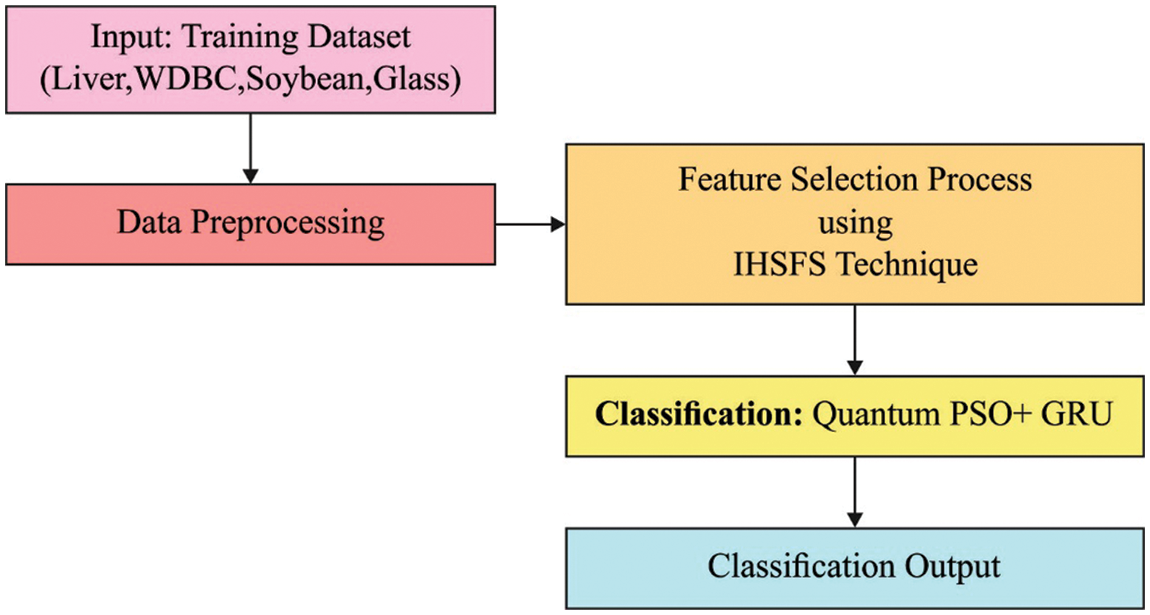
Figure 1: Overall process of IHSFS-ODL technique

2.1 Pre-Processing

Initially, the Z-score normalization approach is employed. It is a standard and normalization approach which defines a number of standard deviations [16]. It preferably ranges from [−3, +3]. It undergoes normalization of the data for transforming the data with distinct scales to the default scale. For z-score based normalization, the difference of the average population from actual data point and partitioned it using the standard deviation that offers a score ranges between [−3, +3]. Therefore, reflecting how many standard deviations a point is above or below the mean as determined using Eq. (1), where x signifies the value of a specific instance, μ denotes the mean and σ symbolizes the standard deviation.

Z−score=(x−μ)σ(1)

2.2 Design of IHSFS Technique

Next to data pre-processing, the IHSFS technique can be applied for the optimal selection of features from the pre-processed data. During the election of features, the pre-processed data is employed in IHSFS technique for choosing the features. The metaheuristic search on optimization problems that sample rates for the perfect state of harmony by improvising searching method. HS is characterized as a set of solution vector named as a harmony memory (HM), whereby all the individuals (vector or harmony) was analogous to particle in particle swarm optimization (PSO) [17]. HM was initialized by an arbitrary solution vector and has upgraded by all the improvisation by some parameter adjustment. The control parameter is pitch adjustment rate (PAR), bandwidth (BW), and harmony memory consideration rate (HMCR). Optimization with harmony search method is given below

Step1: Initialize Control Parameter

Step2: Initialize HM.

Step3: Estimate efficiency of existing harmony.

Step4: Estimate efficiency of recent sample rated harmony and improvise harmony.

Step5: Check end condition

In the system, the length of harmony is count of samples to be elected from the dataset. It employs real encoding system for representing all the bits of the harmony. For harmony vector depiction, all the bits are assigned with real numbers drawn from the searching with lower limit 1 and upper limit with total number of features (TNF) and rounded to integer value representing the feature index. To harmony calculation, related samples a certain harmony contain, the classification error with samples would be lower. Hence, we assume classification error as the FF. Fitness values of harmony are estimated considering classification error as the FF as follows

Fitness−Vector=fir(V1),fit(V2),L,fif(VHMS)(2)

The current harmony is improvised as for j =1 to NOF, if (rand(O,1)<HMCR)

gnew(j)=gf(3)

whereas g characterizes every sample index and f=1,2,3,⋯,HMS if (rand(O,1)<PAR)

gnew(j)=gnew(j)+BW(4)

elsegnew(j)=LB(j)+rand(O,1)×(UB(j)−LB(j)(5)

Now, the float number optimization approach is utilized to feature depiction. According to the probability of feature in the feature subset, feature index is estimated by the distribution factor in sample ration improvisation as FDjg given below.

FDjg=a∗(PDjPDj+NDj)+(1−(PDj+NDj)max(PDj+NDj))(6)

while PDj, indicates the amount of times feature j comes under better subset (the harmony fitness is better than or equivalent to mean fitness) and NDj, shows the amount of times feature j is come under bad subset (the harmony fitness is lesser than equivalent to mean fitness). The high possibility feature has high chance to come in the last subset. Lastly based on the ending conditions (amount of iterations or tolerable classifier error) improvisation was performed and minimized set of features is carefully chosen from this phase. When fit(gnew(j) is greater than fir (worst) then update harmony as follow

gworst=gnew(7)

After all iterations, the parameter HMCR, PAR, and BW is adopted ad follows

HMCRt=11+e−HMCRt,PARt=11+e−PARt,BVVf=11+e−BWt(8)

with Eq. (7) a sigmoidal transformation is employed to this element for bringing the value into a range. These works show a multi-stage FS method executing the benefits of filter and wrapper methodologies.

In HS technique, the pitch fine-tuning function roles a vital play from the searching method. But, to set an appropriate value of bw is most complex, thus it can be presented a local search approach for replacing the pitch altering function. The local searching work is as follows [18]:

Step1 Choose m harmony vector arbitrarily and define the existing optimum harmony vector xbest from the HM.

Step2 for calculating the mean value of these arbitrarily chosen harmony vectors, the calculation formula is demonstrated as:

x¯j=∑i=1mxji(9)

where xji refers the means jth dimensional of ith harmony vector.

Step3 utilize the present optimum harmony vector xbest and the mean harmony vector x¯ for searching a novel harmony vector xnew that work as follows:

Xjnew=xJnew+rand1×(xJbest−round(1+rand2)×x¯j)(10)

where rand1 and rand2 refers the arbitrary number amongst zero and one correspondingly; round signifies the get near integer. Fig. 2 demonstrates the flowchart of HS technique.

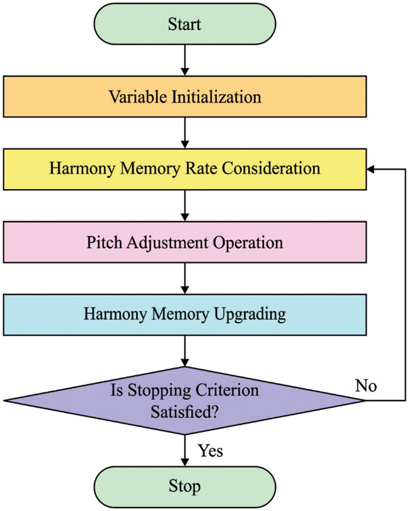
Figure 2: Harmony search flowchart

2.3 Design of QPSO-GRU Classification Model

Once the features are chosen, the classification process is concurrently carried out for every instance using the GRU model. Recurrent neural network (RNN) is most appropriate to process sequential data, however, if the input data is much time, it could not resolve the long-term dependence connection, it is effect gradient explosion or disappearance. The GRU has easier than the infrastructure of long short term memory (LSTM) networks, and their effects are same as LSTM [19]. It can be select the GRU network for learning the time dependence from the signal. Fig. 3 depicts the framework of GRU. There are only 2 gates from the GRU method: the update gate (that is a fusion of forgetting as well as input gates) and reset gate. It can be computed as:

rn=σlog(Wrxn+Urhn−1+br)(11)

zn=σlog(Wzxn+Uzhn−1+bz).(12)

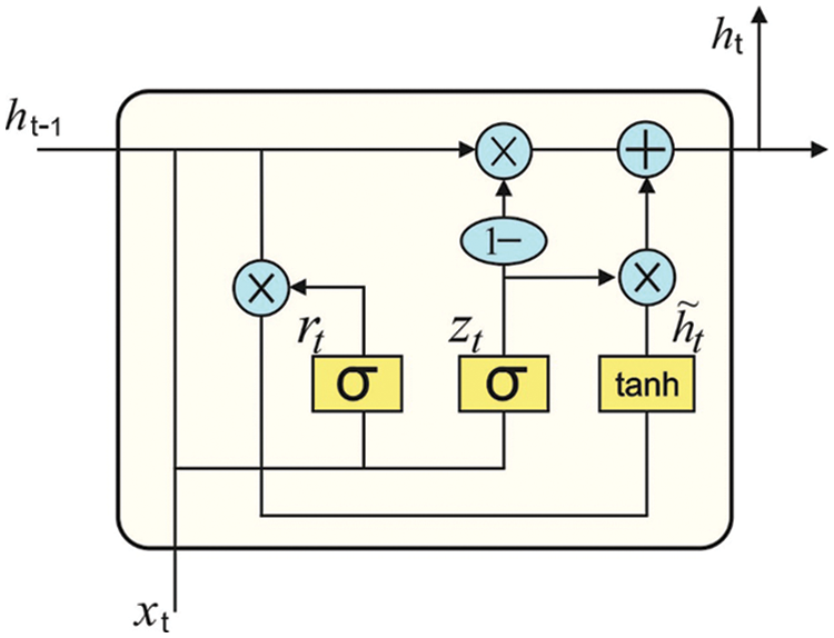
Figure 3: GRU structure

The update gate has been utilized for controlling the extent to that the state data in the preceding moment was carried as to the present state, and reset gate control that several data in the preceding state was expressed as the present candidate set

h~n=tanh⁡(Whxn+Uh(rn∘hn−1)+bh).(13)

hn=zn∘hn−1+(1−z)∘n(14)

where rn implies the reset gate, zn stands for the update gate, xn refers the input vector, hn denotes the hidden state at time n, hn−1 determines the hidden state in the preceding unit, W and U indicates the weighted matrices, b represents the deviation parameters. σlog is the logistic sigmoid function.

In order to determine the hyperparameters of the GRU model, the QPSO algorithm is applied to it. Sun et al. presented a new different of PSO, called QPSO that executes the typical PSO from searching capability [20]. The QPSO algorithm gathers a target point to all the particles; refer Gi= (gi1,gi2,…,giq) as the target point to particles, of that the co-ordinates are

gij=(∅ijpij+(1−φij)pgj,(15)

where (βij) represents the arbitrary number from the interval zero and one. The trajectory study illustrates that Gi is the local attractor of particles; i.e., in PSO, particle i converges to it. The place of particles i has been upgraded as:

xijk+1=gijk±Lijk2ln⁡(1u),(16)

where u implies the arbitrary number from the interval zero and one and C=[c1,c1,…,cq] has recognized as the mean optimum place that is determined as the average of personal optimum place of every particle, so,

cj=1n∑t=1nptj,j=1,2,…,q,(17)

The parameter α is named as Contraction-Expansion Coefficient that is tuned for controlling the convergence speed of techniques. As the iteration of QPSO has been distinct in individuals of PSO, the technique of BPSO could not be executed. The technique of BPSO could not be implemented in QPSO. Sun et al. established the crossover function of genetic algorithm (GA) as to QPSO and presented binary QPSO (BQPSO). During the BQPSO, Xi=(xi1,xi2,…,xiq) until signifies the place of particles i, however, it can be essential for emphasizing that Xi is a binary string before a vector, and xij is that substring of Xi, not the jth bit from the binary string. Consider that the length of all the substrings are l; afterward the length of Xi is lq.

The target point Gi to particles i have been created with crossover function; i.e., BQPSO applies crossover function on the personal optimum place Pi and the global optimum place Pg for generating 2 offspring binary strings, and Gi has arbitrarily chosen in them.

Define

pm=α∗dH(cj,xijk)∗ln⁡(1u),u ∼ U[0,1],(18)

where k refers the amount of iterations and dH(cj,xijk) implies the Hamming distance amongst cj and xijk. Related to the 2-bit strings, the Hamming distance is the amount of bits variance from the 2 strings. cj stands for the jth substring of mean optimum place, and that bit of cj has defined as the states of dth bit of every particle personal optimum places. When further particles get on 1 at the dth bit, the dth bit of cj is 1; then the bit is 0.

To all the bits of gij if pm>rand implement the functions as follows: when the state of the bit is 1, otherwise fixed their state to 0; then set their state to 0. The QPSO method derives a fitness function to accomplish enhanced classification accuracy. It defines a positive integer for representing the good accuracy of the candidate solution. In the study, the minimization of the classification error rate is taken into account as the fitness function, as follows. The optimum solution has a minimum error rate and the worst solution attains an improved error rate.

fitness(xi)=Classifier ErrorRate(xi)=number of misclassified instancesTotal number of instances∗100(19)

3  Experimental Validation

The performance validation of the IHSFS-ODL model is tested using four benchmark datasets [21] namely Liver (345 samples with 6 features), WDBC (569 samples with 30 features), soyabean (685 samples with 35 features), and glass (214 samples with 9 features) datasets.

Tab. 1 and Fig. 4 report the FS results of the IHSFS-ODL model with recent methods. The results indicated that the IHSFS-ODL model has chosen only minimal number of features.

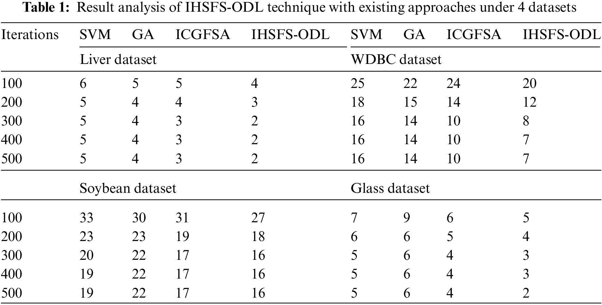
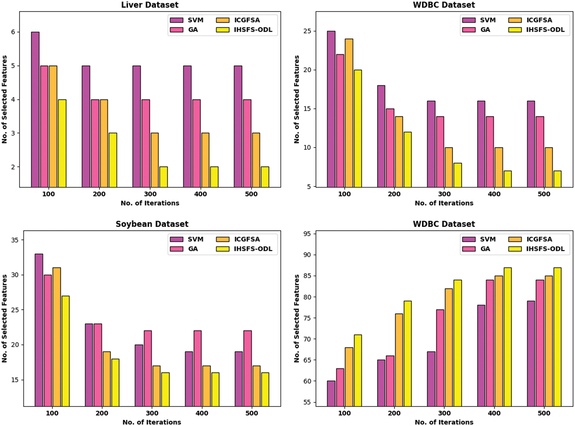
Figure 4: Result analysis of IHSFS-ODL techniques under 4 datasets

For instance, with liver dataset and 100 iterations, the IHSFS-ODL model has derived only 4 features whereas the support vector machine (SVM), GA, and ICGFSA techniques have provided 6, 5, and 5 features respectively. In addition, with WDBC dataset and 100 iterations, the IHSFS-ODL method has derived only 20 features whereas the SVM, GA, and ICGFSA approaches have offered 25, 22, and 24 features correspondingly. Followed by, with soybean dataset and 100 iterations, the IHSFS-ODL algorithm has derived only 27 features whereas the SVM, GA, and ICGFSA techniques have provided 33, 30, and 31 features respectively. In line with, with glass dataset and 100 iterations, the IHSFS-ODL technique has derived only 5 features whereas the SVM, GA, and ICGFSA approaches have provided 7, 9, and 6 features correspondingly.

Tab. 2 and Figs. 5–8 illustrates overall classification results of the IHSFS-ODL model under distinct iterations. The results show that the IHSFS-ODL model has accomplished enhanced classification results on the test datasets applied.

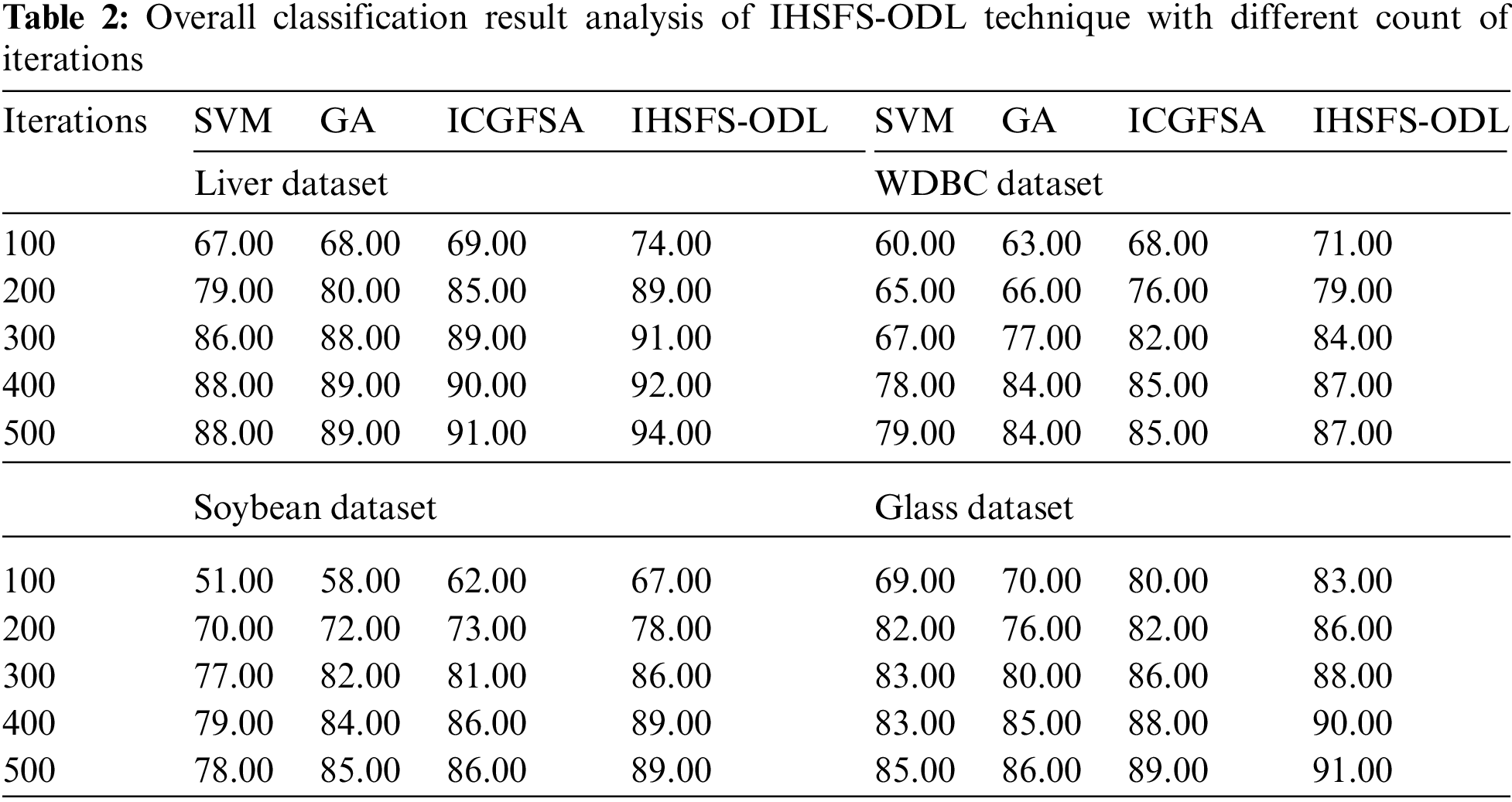
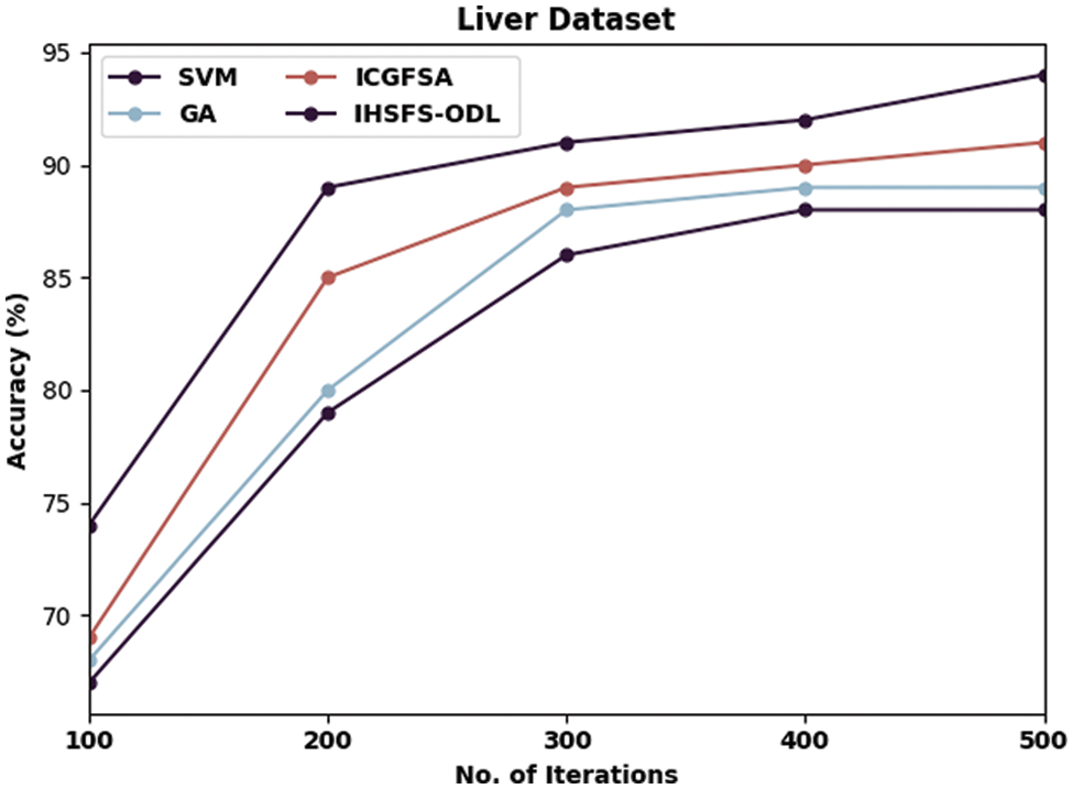
Figure 5: Accuracy analysis of IHSFS-ODL technique under liver dataset

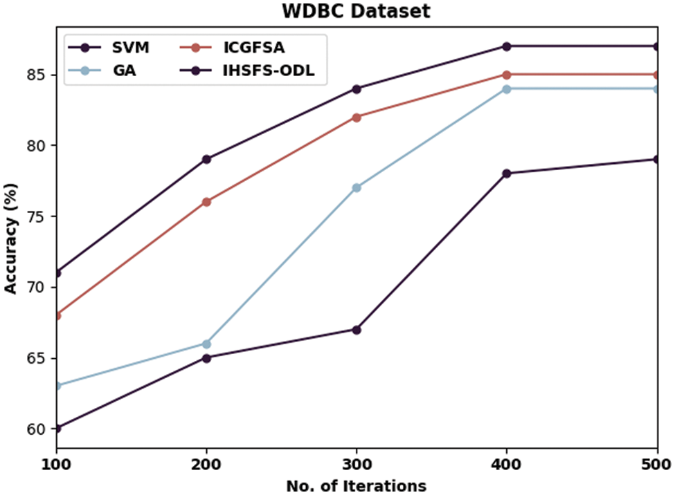
Figure 6: Accuracy analysis of IHSFS-ODL technique under WDBC dataset

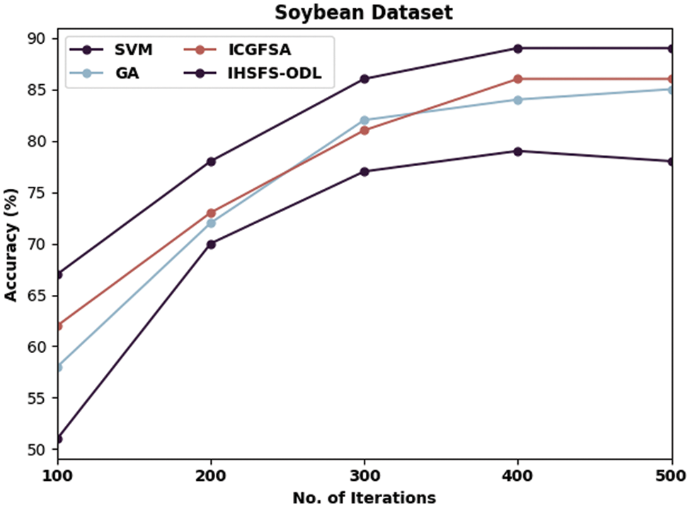
Figure 7: Accuracy analysis of IHSFS-ODL technique under soybean dataset

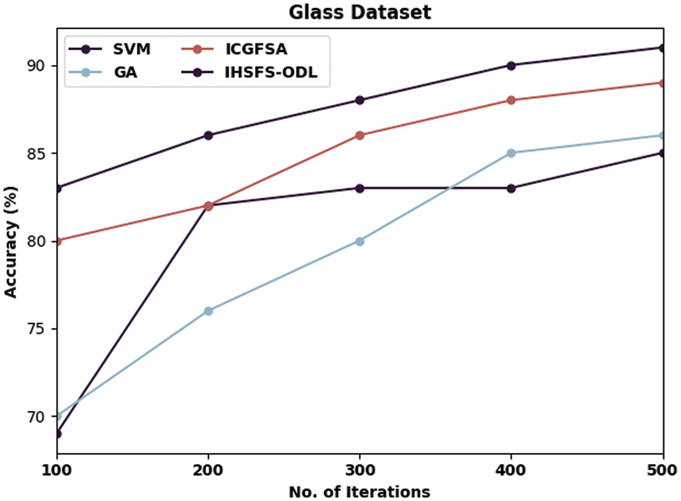
Figure 8: Accuracy analysis of IHSFS-ODL technique under glass dataset

For instance, with liver dataset and 100 iterations, the IHSFS-ODL model has provided higher accuracy of 74% whereas the SVM, GA, and ICGFSA models have accomplished lower accuracy of 67%, 68%, and 69% respectively. Similarly, with 500 iterations, the IHSFS-ODL model has resulted in increased accuracy of 94% whereas the SVM, GA, and ICGFSA models have demonstrated reduced accuracy of 88%, 89%, and 91% respectively.

A detailed running time examination of the IHSFS-ODL model is carried out with recent methods in Tab. 3 and Fig. 9. The experimental results indicated that the IHSFS-ODL model has accomplished minimal running time over other ones. For example, on liver dataset, the IHSFS-ODL model has obtained reduced running time of 0.149 min whereas the SVM, GA, and ICGFSA techniques have offered increased running time of 0.187, 0.185, and 0.205 min respectively. Moreover, on soybean dataset, the IHSFS-ODL method has gained diminished running time of 0.186 min whereas the SVM, GA, and ICGFSA techniques have obtainable higher running times of 0.218, 0.245, and 0.220 min correspondingly. Furthermore, on glass dataset, the IHSFS-ODL technique has obtained minimal running time of 0.190 min whereas the SVM, GA, and ICGFSA approaches have offered increased running time of 0.195, 0.205, and 0.197 min correspondingly.

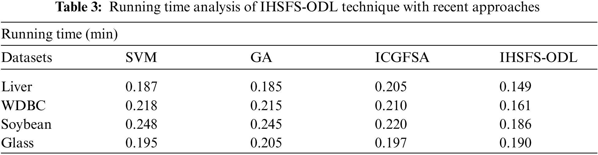
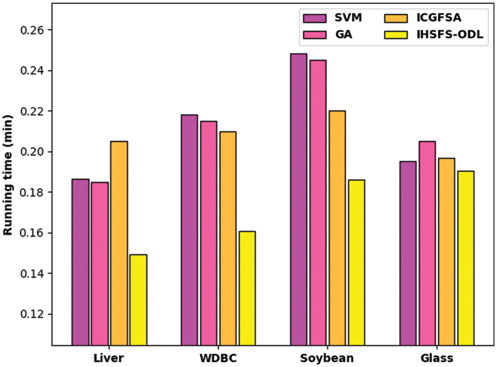
Figure 9: Running time analysis of IHSFS-ODL technique with recent approaches

Similarly, with WDBC dataset and 100 iterations, the IHSFS-ODL algorithm has obtainable superior accuracy of 71% whereas the SVM, GA, and ICGFSA systems have accomplished lower accuracy of 60%, 63%, and 63% respectively. At the same time, with 500 iterations, the IHSFS-ODL system has resulted in maximal accuracy of 87% whereas the SVM, GA, and ICGFSA approaches have outperformed decreased accuracy of 79%, 84%, and 85% correspondingly.

Followed by, with soybean dataset and 100 iterations, the IHSFS-ODL method has provided higher accuracy of 67% whereas the SVM, GA, and ICGFSA approaches have accomplished lower accuracy of 51%, 58%, and 62% respectively. Besides, with 500 iterations, the IHSFS-ODL model has resulted in increased accuracy of 89% whereas the SVM, GA, and ICGFSA models have exhibited lower accuracy of 78%, 85%, and 86% correspondingly.

Lastly, with glass dataset and 100 iterations, the IHSFS-ODL algorithm has provided maximal accuracy of 83% whereas the SVM, GA, and ICGFSA algorithms have accomplished lower accuracy of 69%, 70%, and 80% correspondingly. At last, with 500 iterations, the IHSFS-ODL model has resulted in maximal accuracy of 91% whereas the SVM, GA, and ICGFSA models have demonstrated reduced accuracy of 85%, 86%, and 89% correspondingly.

Finally, the end FS results of the IHSFS-ODL model are examined with recent methods [22] as demonstrated in Tab. 4 and Fig. 10. The results show that the IHSFS-ODL model has accomplished effectual outcomes with less number of chosen features. For instance, on Liver dataset, the IHSFS-ODL model has elected 2 features whereas the SVM, GA, and ICGFSA techniques have chosen 5, 4, and 3 features respectively. In addition, on WDBC dataset, the IHSFS-ODL method has elected 7 features whereas the SVM, GA, and ICGFSA algorithms have chosen 16, 14, and 10 features correspondingly. Along with that, on Glass dataset, the IHSFS-ODL technique has elected 2 features whereas the SVM, GA, and ICGFSA systems have chosen 5, 6, and 4 features correspondingly.

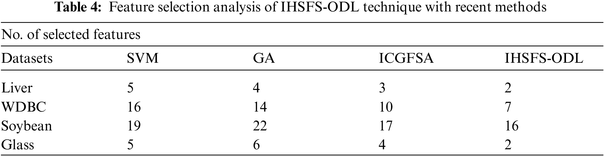
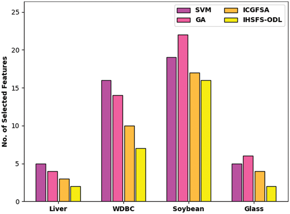
Figure 10: FS analysis of IHSFS-ODL technique with recent methods

From the above mentioned results and discussion, it is evident that the IHSFS-ODL model has resulted in maximum classification results over the other existing techniques.

4  Conclusion

This article has developed a new IHSFS-ODL technique in order to reduce the curse of dimensionality and enhance classification outcomes. The proposed IHSFS-ODL technique contains distinct operations namely Z-score normalization, IHSFS based choice of features, GRU based classification, and QPSO based hyperparameter optimization. The utilization of HSA for the choice of features and QPSO algorithm for hyper parameter tuning processes helps to accomplish maximum classification performance. In order to demonstrate the enhanced outcomes of the IHSFS-ODL technique, a series of simulations were carried out and the results reported the betterment over its recent state of art approaches. Therefore, the IHSFS-ODL technique can be utilized as a proficient tool for global optimization processes. In future, hybrid DL models can be introduced to enhance the classification outcome.

Acknowledgement: This work was funded by the Deanship of Scientific Research (DSR), King Abdulaziz University, Jeddah, under Grant No. (D-914-611-1443). The authors, therefore, gratefully acknowledge DSR technical and financial support.

Funding Statement: This work was funded by the Deanship of Scientific Research (DSR), King Abdulaziz University, Jeddah, under Grant No. (D-914-611-1443).

Conflicts of Interest: The authors declare that they have no conflicts of interest to report regarding the present study.

References

 1.  B. Ghaddar and J. Naoum-Sawaya, “High dimensional data classification and feature selection using support vector machines,” European Journal of Operational Research, vol. 265, no. 3, pp. 993–1004, 2018. [Google Scholar]

 2.  J. Cai, J. Luo, S. Wang and S. Yang, “Feature selection in machine learning: A new perspective,” Neurocomputing, vol. 300, pp. 70–79, 2018. [Google Scholar]

 3.  W. Sun, G. Z. Dai, X. R. Zhang, X. Z. He and X. Chen, “TBE-Net: A three-branch embedding network with part-aware ability and feature complementary learning for vehicle re-identification,” IEEE Transactions on Intelligent Transportation Systems, pp. 1–13, 2021. https://doi.org.10.1109/TITS.2021.3130403. [Google Scholar]

 4.  W. Sun, L. Dai, X. R. Zhang, P. S. Chang and X. Z. He, “RSOD: Real-time Small object detection algorithm in UAV-based traffic monitoring,” Applied Intelligence, vol. 92, no. 6, pp. 1–16, 2021. [Google Scholar]

 5.  A. Chaudhuri and T. P. Sahu, “A hybrid feature selection method based on Binary Jaya algorithm for micro-array data classification,” Computers & Electrical Engineering, vol. 90, no. 12, pp. 106963, 2021. [Google Scholar]

 6.  A. Behura, “The cluster analysis and feature selection: Perspective of machine learning and image processing,” Data Analytics in Bioinformatics: A Machine Learning Perspective, pp. 249–280, 2021. [Google Scholar]

 7.  L. M. Zambrano, K. K. Hadziabdic, T. L. Turukalo, P. Przymus, V. Trajkovik et al., “Applications of machine learning in human microbiome studies: A review on feature selection, biomarker identification, disease prediction and treatment,” Frontiers in Microbiology, vol. 12, pp. 1–25, 2021. [Google Scholar]

 8.  E. O. Omuya, G. O. Okeyo and M. W. Kimwele, “Feature selection for classification using principal component analysis and information gain,” Expert Systems with Applications, vol. 174, pp. 114765, 2021. [Google Scholar]

 9.  D. Tripathi, D. R. Edla, A. Bablani, A. K. Shukla and B. R. Reddy, “Experimental analysis of machine learning methods for credit score classification,” Progress in Artificial Intelligence, vol. 10, no. 3, pp. 217–243, 2021. [Google Scholar]

10. Y. Xue, Y. Tang, X. Xu, J. Liang and F. Neri, “Multi-objective feature selection with missing data in classification,” IEEE Transactions on Emerging Topics in Computational, vol. 6, no. 2, pp. 1–10, 2022. [Google Scholar]

11. N. Nahar, F. Ara, M. Neloy, A. Istiek, A. Biswas et al., “Feature selection based machine learning to improve prediction of parkinson disease,” in Int. Conf. on Brain Informatics, Cham, Lecture Notes in Computer Science book series (LNCSSpringer, 12960, pp. 496–508, 2021. [Google Scholar]

12. R. Aggrawal and S. Pal, “Sequential feature selection and machine learning algorithm-based patient’s death events prediction and diagnosis in heart disease,” SN Computer Science, vol. 1, no. 6, pp. 344, 2020. [Google Scholar]

13. T. Zhang, T. Zhu, P. Xiong, H. Huo, Z. Tari et al., “Correlated differential privacy: Feature selection in machine learning,” IEEE Transactions on Industrial Informatics, vol. 16, no. 3, pp. 2115–2124, 2020. [Google Scholar]

14. K. L. Chiew, C. L. Tan, K. Wong, K. S. C. Yong and W. K. Tiong, “A new hybrid ensemble feature selection framework for machine learning-based phishing detection system,” Information Sciences, vol. 484, no. 13, pp. 153–166, 2019. [Google Scholar]

15. A. Khamparia, A. singh, D. Anand, D. Gupta, A. Khanna et al., “A novel deep learning-based multi-model ensemble method for the prediction of neuromuscular disorders,” Neural Computing and Applications, vol. 32, no. 15, pp. 11083–11095, 2020. [Google Scholar]

16. U. Ahmed, R. Mumtaz, H. Anwar, A. A. Shah, R. Irfan et al., “Efficient water quality prediction using supervised machine learning,” Water, vol. 11, no. 11, pp. 2210, 2019. [Google Scholar]

17. M. Mahdavi, M. Fesanghary and E. Damangir, “An improved harmony search algorithm for solving optimization problems,” Applied Mathematics and Computation, vol. 188, no. 2, pp. 1567–1579, 2007. [Google Scholar]

18. G. Li and H. Wang, “Improved harmony search algorithm for global optimization,” in 2018 Chinese Control and Decision Conf. (CCDC), Shenyang, pp. 864–867, 2018. [Google Scholar]

19. S. V. Karthy, T. S. Kumar and L. Parameswaran, “LSTM and GRU deep learning architectures for smoke prediction system in indoor environment,” in Intelligence in Big Data Technologies—Beyond the Hype, Advances in Intelligent Systems and Computing Book Series (AISC). Vol. 1167. Singapore: Springer, pp. 53–64, 2020 [Google Scholar]

20. T. Sun and M. Xu, “A swarm optimization genetic algorithm based on quantum-behaved particle swarm optimization,” Computational Intelligence and Neuroscience, vol. 2017, no. 3, pp. 1–15, 2017. [Google Scholar]

21. https://archive.ics.uci.edu/ml/index.php. [Google Scholar]

22. S. Wu, Y. Hu, W. Wang, X. Feng and W. Shu, “Application of global optimization methods for feature selection and machine learning,” Mathematical Problems in Engineering, vol. 2013, pp. 1–8, 2013. [Google Scholar]

This work is licensed under a Creative Commons Attribution 4.0 International License, which permits unrestricted use, distribution, and reproduction in any medium, provided the original work is properly cited.