Computers, Materials & Continua DOI:10.32604/cmc.2022.029140
Article

Optimal Fusion-Based Handcrafted with Deep Features for Brain Cancer Classification

Mahmoud Ragab1,2,3,*, Sultanah M. Alshammari4, Amer H. Asseri2,5 and Waleed K. Almutiry6

1Information Technology Department, Faculty of Computing and Information Technology, King Abdulaziz University, Jeddah, 21589, Saudi Arabia
2Center for Artificial Intelligence in Precision Medicines, King Abdulaziz University, Jeddah, 21589, Saudi Arabia
3Mathematics Department, Faculty of Science, Al-Azhar University, Naser City, 11884, Cairo, Egypt
4Computer Science Department, Faculty of Computing and Information Technology, King Abdulaziz University, Jeddah, 21589, Saudi Arabia
5Biochemistry Department, Faculty of Science, King Abdulaziz University, Jeddah, 21589, Saudi Arabia
6Department of Mathematics, College of Science and Arts in Ar Rass, Qassim University, Buryadah, 52571, Saudi Arabia
*Corresponding Author: Mahmoud Ragab. Email: mragab@kau.edu.sa
Received: 25 February 2022; Accepted: 06 April 2022

Abstract: Brain cancer detection and classification is done utilizing distinct medical imaging modalities like computed tomography (CT), or magnetic resonance imaging (MRI). An automated brain cancer classification using computer aided diagnosis (CAD) models can be designed to assist radiologists. With the recent advancement in computer vision (CV) and deep learning (DL) models, it is possible to automatically detect the tumor from images using a computer-aided design. This study focuses on the design of automated Henry Gas Solubility Optimization with Fusion of Handcrafted and Deep Features (HGSO-FHDF) technique for brain cancer classification. The proposed HGSO-FHDF technique aims for detecting and classifying different stages of brain tumors. The proposed HGSO-FHDF technique involves Gabor filtering (GF) technique for removing the noise and enhancing the quality of MRI images. In addition, Tsallis entropy based image segmentation approach is applied to determine injured brain regions in the MRI image. Moreover, a fusion of handcrafted with deep features using Residual Network (ResNet) is utilized as feature extractors. Finally, HGSO algorithm with kernel extreme learning machine (KELM) model was utilized for identifying the presence of brain tumors. For examining the enhanced brain tumor classification performance, a comprehensive set of simulations take place on the BRATS 2015 dataset.

Keywords: Brain cancer; medical imaging; deep learning; fusion model; metaheuristics; feature extraction; handcrafted features

1  Introduction

The death rate because of brain cancer is the maximum in Asia [1]. Brain cancer grows in the spinal cord or brain [2]. The many symptoms of brain cancer involve frequent headaches, coordination issues, changes in speech, mood swings, seizures, memory loss, and difficulty in concentration. Brain cancer is a type of cancer that remains in the central nervous system or brain [3]. It can be classified as to distinct types based on the origin, nature, progression stage, and rate of growth [4]. Either, it is benign or malignant. Benign brain cancer cells hardly attack adjacent healthy cells, have a slower progression rate (for example, pituitary cancers, meningiomas, astrocytoma), and dissimilar boundaries. Malignant brain cancer cells (for example higher-grade astrocytoma, oligodendrogliomas, and so on) willingly invade adjacent cells in the spinal cord or brain, have rapid progression rates and fuzzy borders [5]. Further, it is categorized into two kinds according to the origin: primary and secondary brain cancers.

Primary cancer directly originates in the brain. When cancer develops in the brain because of cancer present in some other body organs like stomach, lungs, and so on, also it is called a metastasis or secondary brain cancer. Furthermore, grading of brain cancer can be performed according to the growth rate of tumorous cells. Also, Brain cancer is considered by the progression phases (Stage-0, 1, 2, 3, and 4). Stage-0 represents tumorous cancer cells that are abnormal, however, it doesn’t spread to neighboring cells [6]. Stages-1, 2, and 3 denote cells that are tumorous and spread quickly. Lastly, in Stage-4 cancer spread all over the body. It is certain that a considerable number of people were saved when cancer was identified at an earlier phase via cost-effective and fast diagnoses methods [7]. But it is complex for treating cancer at the highest stage where the survival rate is lower. The imaging modalities like magnetic resonance imaging (MRI), or computed tomography (CT) of the brain are safer and faster methods when compared to biopsy. This imaging modality assists radiotherapists to observe disease progression, discover brain disorders, and in operational procedures [8].

Brain image reading or brain scans to cure disorder is subjected to inter-reader accuracy and variability based on the ability of the doctor [9]. Various studies have been conducted for developing a robust and accurate solution for the automated classification of brain cancer. But, because of higher inter and intra contrast, shape, and texture dissimilarities, it remains a challenge. The conventional machine learning (ML) method is based on hand-engineered features that restrain the strength of the solution. While the deep learning-based approach extracts useful features that provide good results [10]. Deep learning (DL)-based technique requires a huge number of interpreted information for training, and acquiring this information is a difficult process. Kang et al. [11] presented a technique to brain tumor classifier utilizing an ensemble of deep feature and ML techniques. During this presented structure, can be adapted the model of transfer learning utilizes a different pre-trained deep convolutional neural network (DCNN) for extracting deep features in brain MRI. The extracting deep feature is then estimated by different ML techniques.

The authors in [12] established a multi-level attention process to the task of brain tumor detection. The presented multi-level attention network (MANet) comprises both spatial and cross-channel attention that not only efforts on prioritized tumor region. The authors in [13] presented a novel technique that utilizes DCNNs to classify brain tumors as normal and 3 distinct varieties. The tumor has primarily segmented in the MRI utilizing an improved Independent Component Analysis (ICA) mixture mode method. From the segmentation image, deep feature is extracted and classified. The authors in [14] concentrated on a 3-class classifier problem for distinguishing amongst glioma, meningioma, and pituitary tumors that procedure 3 prominent varieties of brain tumor. The presented classifier method adapts the model of deep transfer learning (TL) and utilizes a pre-trained GoogLeNet for extracting features in brain MRI images.

The authors in [15] presented an intelligent diagnostic model to initial recognition of brain tumor dependent upon radial basis function neural network (RBFNN) and effective deep feature of MRI scan. During the segmentation element, Grab cut approach was executed to segment the tumor region. During the feature extracting component, a CNN was employed to extract of novel deep feature in a segmented image. The extracting deep feature is fed as to RBFNN from the classifier modules. Devnath et al. [16] present a method for automatically detecting pneumoconiosis utilizing a deep features based binary classification. A CNN technique pre-trained with TL in a CheXNet method is primarily utilized for extracting deep features in the X-Ray image, afterward, the deep feature is mapped to high dimension feature space to classifier utilizing SVM and CNN based feature aggregation techniques.

This study focuses on the design of automated Henry Gas Solubility Optimization with Fusion of Handcrafted and Deep Features (HGSO-FHDF) technique for brain cancer classification. The proposed HGSO-FHDF technique involves Gabor filtering (GF) technique for removing the noise and enhancing the quality of the MRI images. In addition, Tsallis entropy based image segmentation approach is applied to determine injured brain regions in the MRI image. Moreover, a fusion of handcrafted with deep features using Residual Network (ResNet) is utilized as feature extractors. Finally, HGSO algorithm with kernel extreme learning machine (KELM) model was utilized for identifying presence of brain tumors. For examining the enhanced brain tumor classification performance, a comprehensive set of simulations take place on the BRATS 2015 dataset.

2  The Proposed HGSO-FHDF Model

In this study, a new HGSO-FHDF technique has been developed for the identification and classification of brain cancer. The presented HGSO-FHDF technique comprises several steps (as shown in Fig. 1) such as GF based pre-processing, Tsallis segmentation, fusion based feature extraction, KELM classifier, and HGSO based parameter optimization. At the final stage, the HGSO algorithm with KELM model was utilized for identifying presence of brain tumors.

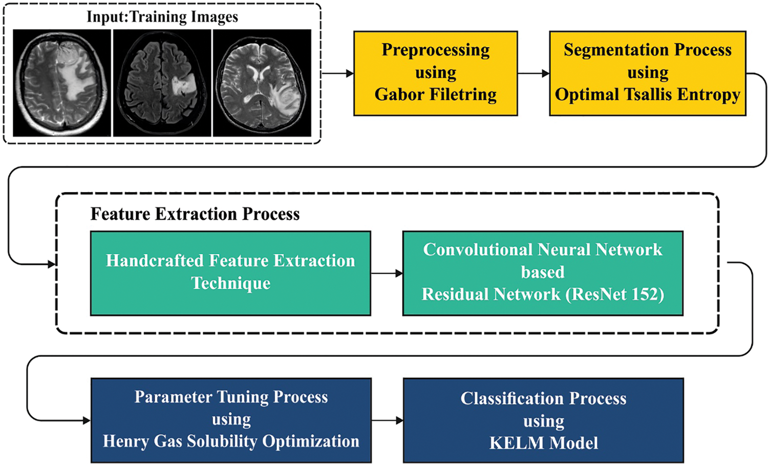
Figure 1: Overall workflow of the proposed model

2.1 Image Pre-processing Using GF Technique

At the primary stage, the input images are preprocessed by the use of GF technique. Gabor transform has a unique biological background. The Gabor filter is the same as the direct representation and frequency of the human visual scheme in terms of direction and frequency, also extracting local data of distinct directions, frequencies, and spatial positions of an image. A main benefit of GF is invariant to translation, scale, and rotation. The purpose why Gabor wavelet is utilized for facial expression detection is that once expression change occurs, the main portions of the face like eyebrows, eyes, and mouth undergoes great change because of muscle change. This part is reflected in the image as grayscale changes. Now, the real and imaginary portions of the wavelet vary, hence the amplitude response of the GF would be very clear, hence it is better suited for extracting local features. In image processing, 2D Gabor filtering is commonly utilized for processing the image. The kernel function of the 2D Gabor wavelet is given as follows:

ψuv(z)=||kuv||2σ2×e||kuv||2||z||22σ2×(eikuvZ−eσ22)(1)

Whereas u and v represents the direction and frequency of Gabor wavelet kernel, z=(x,y) signifies the location of pixel in an image, σ signifies the filter bandwidth, and |kuv|2/σ2 is utilized for compensating the attenuation of energy spectrum defined by the frequency. The Gabor feature of the image is attained by convolving the Gabor wavelet kernel and the facial expression image. Assume that the gray values of (x,y) point in the facial expression image is fixed to k, it can be expressed as follows

Guv(x,y)=I(x,y)∗ψuv(x,y)(2)

Whereas Guv(x,y) denotes the Gabor feature of the extracted image, ψUV(x,y) denotes the kernel function of 2S Gabor wavelet, and ∗ indicates the convolutional process.

2.2 Tsallis Entropy Based Segmentation

Here, Tsallis entropy is applied to segment the affected regions. The entropy is related to the chaos metric in the system. Primarily, Shannon indicated that when the physical systems are separated into 2 statistical free subsystem A & B, entropy value can be defined as follows:

S(A+B)=S(A)+S(B)(3)

Based on Shannon concept, a non-extensive entropy concept is derived as given below.

Sq=1−∑i=1T(pi)qq−1(4)

where T signifies the system potential, q designates the entropic index, and pi denotes likelihood of every state i. The Tsallis entropy Sq satisfies Shannon entropy by q→1. The entropy value is defined by the use of pseudo additive rule as given below:

Sq(A+B)=Sq(A)+Sq(B)+(1−q).Sq(A).Sq(B)(5)

The Tsallis entropy is employed for identifying optimal thresholds of the images. Consider L gray levels in the interval {0,1,…,L−1} with probability distribution pi=p0,p1,…,pL−1. So, the Tsallis multilevel thresholding is defined using following equations.

[SqA(T)+SqB(T)+…+SqK(T)+(1−q).SqA(T).SqB(T)…SqK(T)](6)

whereas

SqA(T)=1−∑i=0t1−1(PiPA)qq−1,PA=∑i=0t1−1Pi

SqB(T)=1−∑i=t1t2−1(PPB)qq−1,PB=∑i=t1t2−1Pi

SqK(T)=1−∑i=tk−1L−1(PiPK)qq−1,PK=∑i=tk−1L−1Pi

2.3 Feature Extraction

At the time of feature extraction, a fusion of handcrafted features using LDEP and deep features using ResNet-152 model are fused together to generate feature vectors. The whole procedure of computation of the LDEPi,j’ for center pixel Ii,j. Consider Qni,j denoted the nth diagonal neighbor of center pixel Qi,j at the distance D from a center pixel Qi,j, consider n∈[1,4] and Qi,j indicates the pixel at ith row and jth column of gray-scaled image M have m1 rows and m2 columns. Where Ini,j and Ii,j denotes the intensity value of Qni,j and Qi,j, correspondingly [17].

τmax=arg⁡max(sign(α)=0∀α∈[0,2])(7)

τmin=arg⁡min(sign(α)=0∀α∈[0,2])(8)

whereas,

sign(α)={1α≥00α<0}(9)

The values of LDEPnij˙ and is determined below.

LDEPni,j={1,if n=(τmax+8ω)orn=(τmin+4+8ω)0,otherwise(10)

At last, the LDEPni,j denotes the pattern calculated over an image of size m1Xm2 as follows

LDEPni,j(m1×m2)=(LDEP1i,j,LDEP2i,j,⋯,LDEPdimi,j)(11)

ResNet comprises a residual learning unit in resolving the weakening of DL models. It enables to allow the inclusion of new inputs and outputs [18]. Fig. 2 shows the structure of residual blocks. A major benefit is an improvement in classifier results with no inclusion of model complexities. The ResNet152 model has been developed by the integration of 3-layer blocks, which is less complicated compared to other models. The connections among the residual block are advantages. It helps to maintain the data attained via training and improves model building time.

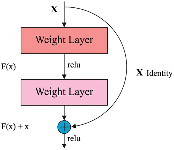
Figure 2: Structure of Residual Blocks

2.4 KELM Based Classification

Next to feature extraction process, the KELM model has been developed for the identification of breast cancer [19]. An extreme learning machine (ELM) resultant function under the case of single resultant node is:

f(x)=∑i=1LβiG(ai,bi,x)=β⋅h(x)(12)

where is the resultant weight amongst the ith node of hidden and output states and β=[β1,…,βL]T represents the resultant weight vector. G(ai,bi,x) signifies the output of ith hidden state node and the node parameter has arbitrarily created. h(x)=[G(a1,b1,x),…,G(aL,bL,x)]T signifies the resultant vector of hidden state comparative to input. Then introduced the kernel function, the kernel matrix of KELM is determined as:

ΩELM=HHT:ΩELM=h(xi)⋅h(xj)=K(xi,xj)(13)

The resultant function of ELM classification is more expressed as:

=[K(x,x1)⋮K(x,xN)](Iλ+ΩELM)−1T(14)

where I refers the identity matrix, λ implies the regularized co-efficient, and T stands for the trained set label. Afterward, it can utilize this technique, it does not require knowing the particular method of feature map h(x) then utilizing the kernel function for resultant calculation.

2.5 Optimal Parameter Adjustment Using HGSO Algorithm

At the final stage, the HGSO algorithm has been employed to optimally tune the parameters involved in it [20]. According to Henry’s law, it reproduces the huddling performance of gas for balancing exploitation as well as exploration from the searching space and avoiding local optimum. The core functions needed for this work are listed as follows. Henry’s co-efficient is computed utilizing in Eq. (15).

Hj(m+1)=Hj(m)⋅exp⁡(−Cj⋅(1/T(m)−1/Tθ)).(15)

where T(m) refers the temperature of mth generation. T(m)=exp⁡(−m/MaxIter). Tθ=298.15. The population has been separated as to equivalent clusters corresponding to the amount of gas types. All the clusters share the similar Henry’s constant value (Hj). A primary generation co-efficient Hj(1)=0.05⋅rand(). rand() implies the function which creates an arbitrary number amongst zero and one. Another co-efficient Cj=0.01.rand(). The solubility has been obtained utilizing Eq. (15).

Si,j(m)=Ks⋅Hj(m+1)⋅Pi,j(m).(16)

where Si,j(m) signifies the solubility of gas i from the cluster j of mth generation. Ks refer the constant. Pi,j(m) represents the partial pressure on gas i from the cluster j of mth generation. The place here relates to the SVR parameter in this work. This function is very serious and upgrades utilizing in Eq. (17).

η=β⋅exp⁡(−Fopt(m)+0.⋅05Fi,j(m)+005).(17)

where Xi,j(m) denotes the place of gas i from the cluster j of mth generation. Xi,j(m+1) indicates the next place of Xi,j(m). r stands for the arbitrary value amongst zero and one. α=1. β refers the constant. F represents the flag which changes the direction of searching agent and offers diversity =±. Xj,opt(m) defines the optimum gas from the cluster j of mth generation. Xopt(m) demonstrated the optimum gas of mth generation. Fopt(m) signifies the fitness of optimum gas of mth generation. F(m) means the fitness of gas i from the cluster j of mth generation. The rank and choose the amount of worse individuals (Nw) utilizing in Eq. (18).

Nw=n⋅(rand(O.1)+O.1).(18)

Assume that the worse individual recreates in the numerical range utilized in Eq. (19).

Gk=LB+ra.(UB−LB).(19)

where Gk refers the place or worse individuals. 1≤k≤Nw. ra stands for the arbitrary value amongst zero and one.

3  Results and Discussion

The performance validation of the HGSO-FHDF technique is tested using the Figshare dataset [21]. The dataset includes three class labels with 150 images under Meningioma, 150 images under Glioma, and 150 images under Pituitary classes. Fig. 3 demonstrates the sample set of test images.

Fig. 4 highlights the confusion matrices of the HGSO-FHDF model under different hidden layers (HLs). The figure indicated that the HGSO-FHDF model has effectually recognized all the classes under all HLs.

Tab. 1 reports comprehensive classification outcomes of the HGSO-FHDF model under different numbers of hidden layers (HLs). The experimental values denoted that the HGSO-FHDF model has accomplished maximum outcome under all HLs.

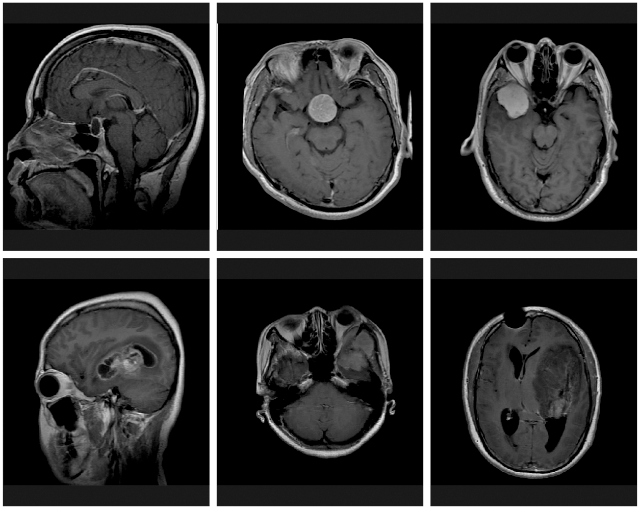
Figure 3: Sample images

Figure 4: Confusion matrices of HGSO-FHDF model

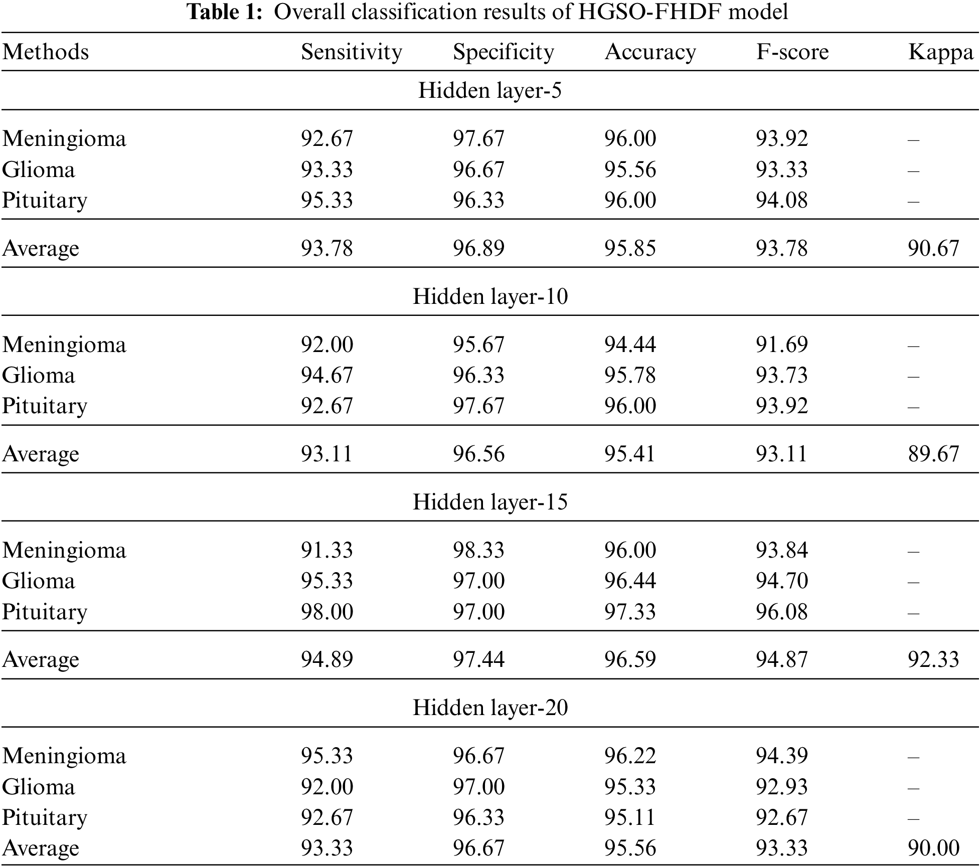
Fig. 5 demonstrates the classifier results of the HGSO-FHDF model under HL of 5. The figure indicated that the HGSO-FHDF model has effectually identified all the classes. For instance, with Meningioma class, the HGSO-FHDF model has offered sensy of 92.67%, specy of 97.67%, accuy of 96%, and Fscore of 93.92% respectively. Along with that, with Glioma class, the HGSO-FHDF model has provided sensy of 93.33%, specy of 96.67%, accuy of 95.56%, and Fscore of 94.08% respectively. Moreover, with Pituitary class, the HGSO-FHDF model has reached sensy of 95.33%, specy of 96.33%, accuy of 96%, and Fscore of 94.08% respectively.

Figure 5: Classification results of HGSO-FHDF model under HL-5

Fig. 6 validates the classifier results of the HGSO-FHDF model under HL of 10. The figure designated that the HGSO-FHDF model has effectively recognized all the classes. For instance, with Meningioma class, the HGSO-FHDF model has presented sensy of 92%, specy of 95.67%, accuy of 94.44%, and Fscore of 91.69% respectively. Also, with Glioma class, the HGSO-FHDF model has provided sensy of 94.67%, specy of 96.33%, accuy of 95.78%, and Fscore of 93.73% respectively. Also, with Pituitary class, the HGSO-FHDF model has reached sensy of 92.67%, specy of 97.67%, accuy of 96%, and Fscore of 93.92% respectively.

Figure 6: Classification results of HGSO-FHDF model under HL-10

Fig. 7 provides the classification outcomes of the HGSO-FHDF model under HL of 10. The figure designated that the HGSO-FHDF model has effectively recognized all the classes. For instance, with Meningioma class, the HGSO-FHDF model has presented sensy of 91.33%, specy of 98.33%, accuy of 96%, and Fscore of 93.84% respectively. Likewise, with Glioma class, the HGSO-FHDF model has provided sensy of 95.33%, specy of 97%, accuy of 96.44%, and Fscore of 94.70% respectively. Likewise, with Pituitary class, the HGSO-FHDF model has reached sensy of 98%, specy of 97.00%, accuy of 97.33%, and Fscore of 96.08% respectively.

Figure 7: Classification results of HGSO-FHDF model under HL-15

Fig. 8 showcases the accuracy and loss graphs offered by the HGSO-FHDF technique on the training and validation datasets under varying numbers of hidden layers. The figure portrayed that the HGSO-FHDF technique has resulted in increased accuracy and reduced loss.

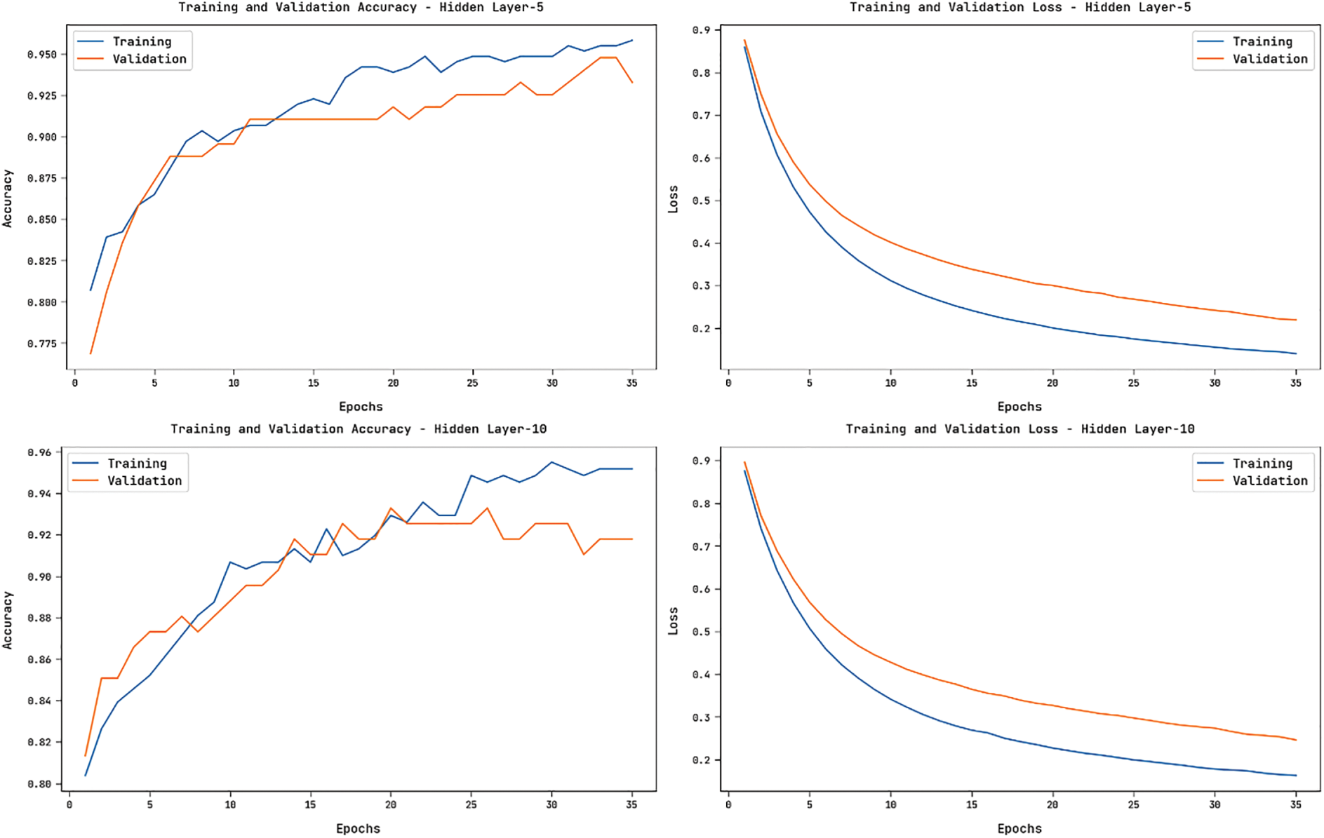
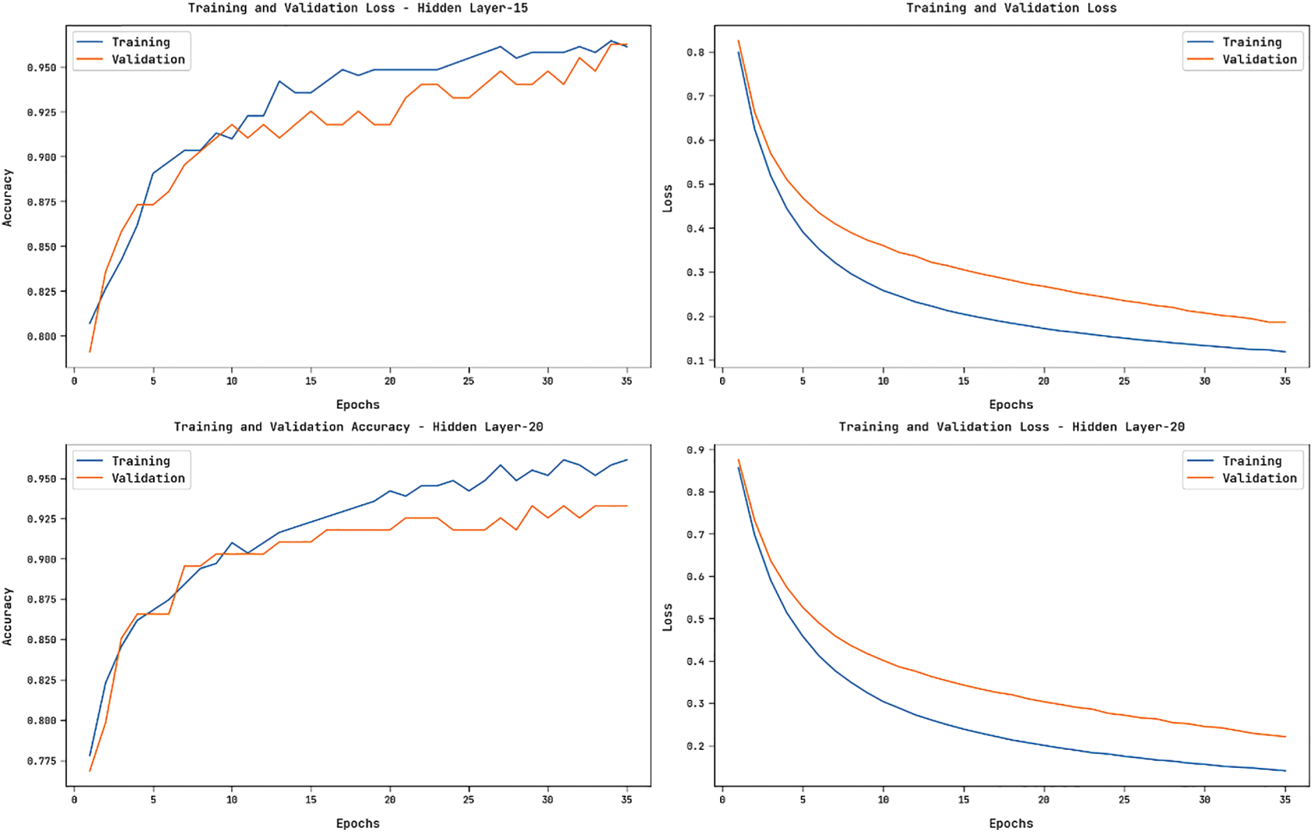
Figure 8: Accuracy and Loss Graph of HGSO-FHDF model

For demonstrating the better outcomes of the HGSO-FHDF technique, a detailed comparison study is made with existing techniques [22] in Tab. 2. Fig. 9 demonstrates the kappa examination of the HGSO-FHDF model with existing techniques. The figure represented that the ResNet50, Inc. V3, and M-Net V2 models have attained lesser kappa values of 90.52%, 88.67%, and 86.67%. Besides, the DNet201 model has resulted in certainly improved kappa value of 90.24%. However, the HGSO-FHDF model has reached better performance with a higher kappa of 92.33%.

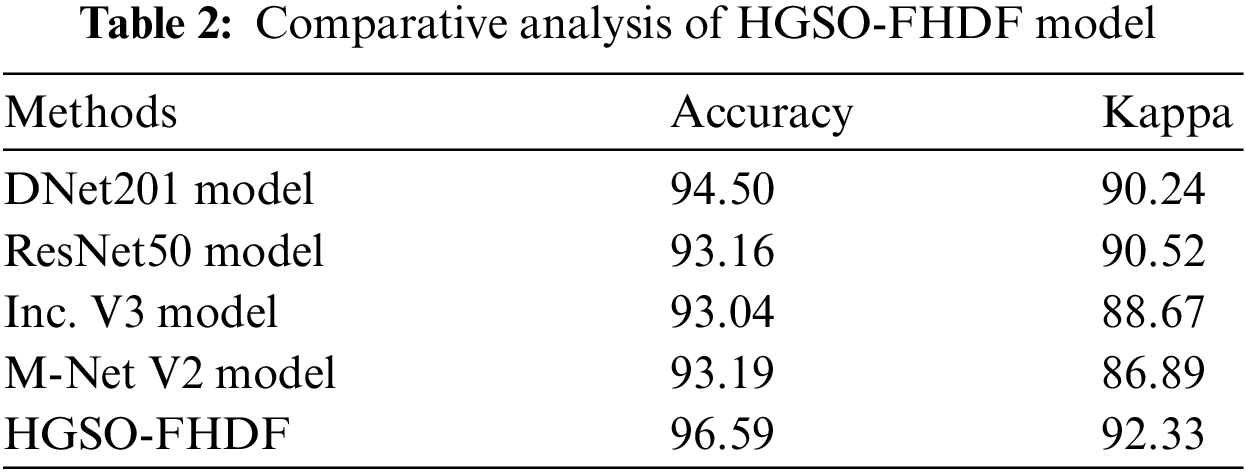
Figure 9: Comparative classification results of HGSO-FHDF model in terms of accuy

Fig. 10 illustrates the accuy investigation of the HGSO-FHDF model with recent methods. The figure portrayed that the ResNet50, Inc. V3, and M-Net V2 models have obtained lower accuy values of 93.16%, 93.04%, and 93.19%. At the same time, the DNet201 model has gained a slightly increased accuy value of 94.50%. However, the HGSO-FHDF model has accomplished a superior outcome with a maximum accuy of 96.59%. The above mentioned tables and figures reported that the HGSO-FHDF model has resulted in maximum classification outcomes over the other methods.

Figure 10: Comparative classification results of HGSO-FHDF model in terms of kappa

4  Conclusion

In this study, a new HGSO-FHDF technique has been developed for the identification and classification of brain cancer. The presented HGSO-FHDF technique comprises GF based pre-processing, Tsallis segmentation, fusion based feature extraction, KELM classifier, and HGSO based parameter optimization. At the final stage, the HGSO algorithm with KELM model was utilized for identifying presence of brain tumors. For examining the enhanced brain tumor classification performance, a comprehensive set of simulations occur on BRATS 2015 dataset. The comparative study of the HGSO-FHDF technique can be utilized as a proficient approach for brain cancer classification. Therefore, the HGSO-FHDF approach is employed as an effective tool for brain cancer detection. In future, advanced DL based segmentation models can be introduced to improve classification results.

Acknowledgement: The authors extend their appreciation to the Deputyship for Research and Innovation, Ministry of Education in Saudi Arabia for funding this research work through the project number (IFPHI- 180-612-2020) and King Abdulaziz University, DSR, Jeddah, Saudi Arabia.

Funding Statement: This research work was funded by Institutional fund projects under grant no. (IFPHI-180-612-2020). Therefore, the authors gratefully acknowledge technical and financial support from the Ministry of Education and King Abdulaziz University, DSR, Jeddah, Saudi Arabia.

Conflicts of Interest: The authors declare that they have no conflicts of interest to report regarding the present study.

References

 1.  G. S. Tandel, M. Biswas, O. G. Kakde, A. Tiwari, H. S. Suri et al., “A review on a deep learning perspective in brain cancer classification,” Cancers, vol. 11, no. 1, pp. 111, 2019. [Google Scholar]

 2.  S. A. A. Ismael, A. Mohammed and H. Hefny, “An enhanced deep learning approach for brain cancer MRI images classification using residual networks,” Artificial Intelligence in Medicine, vol. 102, pp. 101779, 2020. [Google Scholar]

 3.  H. Fabelo, S. Ortega, D. Ravi, B. R. Kiran, C. Sosa et al., “Spatio-spectral classification of hyperspectral images for brain cancer detection during surgical operations,” PLOS ONE, vol. 13, no. 3, pp. e0193721, 2018. [Google Scholar]

 4.  T. Ruba, R. Tamilselvi, M. P. Beham and N. Aparna, “Accurate classification and detection of brain cancer cells in mri and ct images using nano contrast agents,” Biomedical and Pharmacology Journal, vol. 13, no. 3, pp. 1227–1237, 2020. [Google Scholar]

 5.  X. R. Zhang, X. Sun, W. Sun, T. Xu and P. P. Wang, “Deformation expression of soft tissue based on BP neural network,” Intelligent Automation & Soft Computing, vol. 32, no. 2, pp. 1041–1053, 2022. [Google Scholar]

 6.  X. R. Zhang, J. Zhou, W. Sun and S. K. Jha, “A lightweight CNN based on transfer learning for COVID-19 diagnosis,” Computers Materials & Continua, vol. 72, no. 1, pp. 1123–1137, 2022. [Google Scholar]

 7.  F. E. Hakym and B. Mahi, “Brain cancer ontology construction,” in Int. Conf. on Business Intelligence, Lecture Notes in Business Information Processing book series, Cham, Springer, pp. 379–387, 2021. [Google Scholar]

 8.  E. Irmak, “Multi-classification of brain tumor MRI images using deep convolutional neural network with fully optimized framework,” Iranian Journal of Science and Technology-Transactions of Electrical Engineering, vol. 45, no. 3, pp. 1015–1036, 2021. [Google Scholar]

 9.  C. S. Rao and K. Karunakara, “A comprehensive review on brain tumor segmentation and classification of MRI images,” Multimedia Tools and Applications, vol. 80, no. 12, pp. 17611–17643, 2021. [Google Scholar]

10. N. Bacanin, T. Bezdan, K. Venkatachalam and F. A. Turjman, “Optimized convolutional neural network by firefly algorithm for magnetic resonance image classification of glioma brain tumor grade,” Journal of Real-Time Image Processing, vol. 18, no. 4, pp. 1085–1098, 2021. [Google Scholar]

11. J. Kang, Z. Ullah and J. Gwak, “MRI-based brain tumor classification using ensemble of deep features and machine learning classifiers,” Sensors, vol. 21, no. 6, pp. 2222, 2021. [Google Scholar]

12. N. S. Shaik and T. K. Cherukuri, “Multi-level attention network: application to brain tumor classification,” Signal Image and Video Processing, vol. 16, pp. 817–824, 2021. [Google Scholar]

13. S. Basheera and M. S. S. Ram, “Classification of brain tumors using deep features extracted using CNN,” Journal of Physics: Conference Series, vol. 1172, pp. 012016, 2019. [Google Scholar]

14. S. Deepak and P. M. Ameer, “Brain tumor classification using deep CNN features via transfer learning,” Computers in Biology and Medicine, vol. 111, no. 3, pp. 103345, 2019. [Google Scholar]

15. A. Addeh and M. Iri, “Brain tumor type classification using deep features of MRI images and optimized RBFNN,” ENG Transactions, vol. 2, pp. 1–7, 2021. [Google Scholar]

16. L. Devnath, S. Luo, P. Summons and D. Wang, “Automated detection of pneumoconiosis with multilevel deep features learned from chest X-Ray radiographs,” Computers in Biology and Medicine, vol. 129, pp. 104125, 2021. [Google Scholar]

17. S. J. Narayanan, R. Soundrapandiyan, B. Perumal and C. J. Baby, “Emphysema medical image classification using fuzzy decision tree with fuzzy particle swarm optimization clustering,” in Smart Intelligent Computing and Applications, Smart Innovation, Systems and Technologies book series. Singapore, Springer, Vol. 104, pp. 305–313, 2019. [Google Scholar]

18. X. Xu, W. Li and Q. Duan, “Transfer learning and SE-ResNet152 networks-based for small-scale unbalanced fish species identification,” Computers and Electronics in Agriculture, vol. 180, pp. 105878, 2021. [Google Scholar]

19. J. Li, C. Hai, Z. Feng and G. Li, “A transformer fault diagnosis method based on parameters optimization of hybrid kernel extreme learning machine,” IEEE Access, vol. 9, pp. 126891–126902, 2021. [Google Scholar]

20. W. Cao, X. Liu and J. Ni, “Parameter optimization of support vector regression using henry gas solubility optimization algorithm,” IEEE Access, vol. 8, pp. 88633–88642, 2020. [Google Scholar]

21. J. Cheng, “Brain tumor dataset,” Figshare, 2017. https://figshare.com/articles/dataset/brain_tumor_dataset/1512427. [Google Scholar]

22. T. Sadad, A. Rehman, A. Munir, T. Saba, U. Tariq et al., “Brain tumor detection and multi-classification using advanced deep learning techniques,” Microscopy Research and Technique, vol. 84, no. 6, pp. 1296–1308, 2021. [Google Scholar]

This work is licensed under a Creative Commons Attribution 4.0 International License, which permits unrestricted use, distribution, and reproduction in any medium, provided the original work is properly cited.