Computers, Materials & Continua DOI:10.32604/cmc.2022.029473
Article

Explainable Software Fault Localization Model: From Blackbox to Whitebox

Abdulaziz Alhumam*

Department of Computer Science, College of Computer Sciences and Information Technology, King Faisal University, Al-Ahsa, 31982, Saudi Arabia
*Corresponding Author: Abdulaziz Alhumam. Email: aahumam@kfu.edu.sa
Received: 04 March 2022; Accepted: 14 April 2022

Abstract: The most resource-intensive and laborious part of debugging is finding the exact location of the fault from the more significant number of code snippets. Plenty of machine intelligence models has offered the effective localization of defects. Some models can precisely locate the faulty with more than 95% accuracy, resulting in demand for trustworthy models in fault localization. Confidence and trustworthiness within machine intelligence-based software models can only be achieved via explainable artificial intelligence in Fault Localization (XFL). The current study presents a model for generating counterfactual interpretations for the fault localization model's decisions. Neural system approximations and disseminated presentation of input information may be achieved by building a nonlinear neural network model. That demonstrates a high level of proficiency in transfer learning, even with minimal training data. The proposed XFL would make the decision-making transparent simultaneously without impacting the model's performance. The proposed XFL ranks the software program statements based on the possible vulnerability score approximated from the training data. The model's performance is further evaluated using various metrics like the number of assessed statements, confidence level of fault localization, and Top-N evaluation strategies.

Keywords: Software fault localization; explainable artificial intelligence; statement ranking; vulnerability detection

1  Introduction

Artificial intelligence that can be explained (XAI) is a critical component of boosting public confidence in intelligent machine systems. According to different basic assumptions, these XFL strategies were created to assess the possibility of each statement being erroneous, known as suspiciousness, using various fault locator functions. Software developers focus on the accuracy of their products’ functions since they are so commonplace in our everyday lives. Debugging software has been more challenging over the last several decades as the complexity and volume of software have increased. Large-scale software systems need extensive debugging, even if test results or erroneous behavior suggest that the program is defective [1]. Some combinations of system characteristics are required to disclose these defects, resulting in unpredictable behavior. The interplay between these elements causes the malfunction of the system.

Code faults that affect just very few or maybe even a single statement of code is often the source of issues. Model-based safe development process or current compilations of the good security vulnerabilities and recommendations must be supplemented with analytical quality assurance methods for finding fault in source code to minimize such errors. Due to modern software's rising scale and complexity and the increasing list of possible attacks, human source code vulnerability identification must be backed by automated procedures. These methods may (i) accurately discover possible faulty and (ii) lead programmers to the susceptible code fragments. The strategies should also be (iii) scalable to real-time application software, (iv) generalizable across software projects, and (v) easy to set up or configure. And none of the present approaches meet most of these criteria.

Some of the most common ways for building predictive models for different software engineering activities like fault detection or effort estimate include machine learning techniques. The software intelligence literature's predominant criteria for assessing predictive models is accuracy (as measured by metrics such as precision, recall, F-measure, Mean Absolute Error, and similar). Support Vector Machine (SVM), ensemble approaches, and deep neural networks are sophisticated and complicated models that increase predicted accuracy [2]. It is challenging for software developers to grasp and interpret the predictions made by these “black box” models, which many regarded as difficult to comprehend. Due to a lack of confidence in software analyses due to its lack of interpretability, the industry has been reluctant to accept or use the technology. A model's predictions are worthless if software practitioners don't know how to interpret them. They're also worthless if they have to devote project resources or time to implementing the forecasts. If the model has a good track record of accuracy throughout testing, it might help build confidence. However, when the model is deployed and used “in the wild,” the outcomes may be different. Because the model creator already knows the test data, the “future” data may be radically different from the test data, reducing the prediction machine's usefulness considerably. Model predictions that deviate from the software developer's expectations are particularly critical in establishing trust (e.g., sending alarms for areas of coding that the developer expects to be “clean”) [3]. To build trust with practitioners, an explanation must be clear and concise. However, it's not the only factor in a practitioner's opinion. To fix a bug, generally, the software programmer wants to know how a fault localization model predicts a particular statement is vulnerable. To put it another way, marking a file as “defective” is not always sufficient. Such predictions need those developers to have some trace and rationale for them.

The current study is largely motivated from the conventional fault localization techniques, that ranks the statements based on the probability of being vulnerable. There is a demand for the model that is transparent in assigning the rank and the decision making. Moreover, the feature weight optimization and the normalization that have a significant impact on the performance of the neural network model are being observed and evaluated in the current study. The main objective of the present study is to develop a robust fault localization model whose decisions are interpretable. The proposed model relay on the Explainable Artificial Intelligence framework, where the decisions made by the model are explainable and interpretable to build a trustworthy model. Some of the pivotal objectives of the current study are listed below

■   To design and build a robust model that can assist in localizing the faulty statements associated with the program.

■   The code statements in the software program are associated with the rank that determines the possible vulnerability related to the program statement.

■   The decision model and the probabilistic measures associated with the vulnerability score must be explainable and interpretable for the software professional.

■   The outcome associated with the XFL would be more precise when performing the optimization, the feature weights, and batch normalization.

■   In evaluating the score associated with the statements, the global best and the best score within the program fragment are considered optimal.

■   The statement with the highest score is assumed to be more vulnerable, and by introspecting those statements, the debugging process must be made easy.

The entire study is organized across various sections, where Section 1 elaborates more on the introduction to the field of study and the objectives. Section 2 is the literature review where various existing models are discussed in line with the proposed model. Section 3 elaborates more on the background of the study that discusses the XAI-driven feature weight optimization. Section 4 presents the proposed XAI-driven fault localization model and the layered architecture of the deep neural network model. Section 5 focuses on the results and discussion associated with the proposed model, and Section 6 presents the conclusion of the study.

2  Background

XFL algorithms attempt to uncover unknown vulnerabilities over the target software by training numerous vulnerability patterns from pre-existing data. Data collection, model creation, and evaluation are the three most used DLVP procedures. After gathering training data, an appropriate model is chosen depending on the design goal and resource-related constraints. Initially, the training data is processed in the manner suggested by the classifier. After that, the classifier is trained to reduce the loss function. The trained model is employed to use in localization practices.

The majority of the model's design is generated by the data that will be included. Token-based or graph-based models are prominent Deep Learning-based vulnerability detection solutions. The data items are a deep learning-based fault detection model trained on a massive real-time dataset [4]. VUDENC [5] concentrates on a textual way of presenting the source code to ensure readability across a wide range of applications. The vulnerable ranking of the program statements and the fragments are built through a dynamic slice of a failed test case's erroneous output. A dynamic slice comprises an execution log and the stack traces of executed programs. Furthermore, as the program fragmentation criteria, the model employs the program statements with their probabilistic vulnerability rank that highlights the defective statements identified through a failed test case. Those statements might influence subsequent after fault statements [6].

The proposed approach is based on features extracted connected with the valuation process to analyze the software snippet's operating method. As a result, the features are prioritized according to the probability of the fragment failing. The ranks are then utilized to examine the software's design principle and work technique closely. All static and dynamic features were evaluated for fault localization and other extensive feature sets [7]. Across programming languages, the employment of numerous classes, packages, and objects is prevalent. Other aspects are static, while objects are formed at run-time. Their relationship is primarily dynamic [8]. Fig. 1 depicts a few of these correlations.

Figure 1: Image representing the vulnerable statements in association with the test cases

Comprehensive static and dynamic investigation of a software program is required for discovering vulnerable statements in the program. Static analyses describe the system, whereas dynamic analysis profiles the often-utilized parts. These components are the first to be restructured or optimized. The static feature collection consists of a set of parameters associated with the software program that may be vulnerable, resulting in a defect in the program fragment or program malfunction. The feature set is more about the program's information that explains the entire framework, including integer utilization, logic, conditional expressions, statement indentation, labels, and annotations used throughout the program. Static program information preserves the program structure, but even advanced analysis approaches retrieve only a limited amount of knowledge about the program's behavior beforehand. Some of the static features are being presented in Tab. 1 [9].

The associated dynamic features in the software statements are identified by repeated evaluation through the test cases, looking at the program's reaction towards the test cases, and interpreting the stack information to see how the program behaves. The dynamic features, code fragments, and vulnerable statements associated with the software program are recognized through the models. All the statements are classified using an explainable fault localization mechanism. Fig. 2 represents the set of features used in classifying the features as low and highly vulnerable.

Figure 2: Image representing the feature set for fault localization

3  Literature Review

It is necessary to choose input data, execute the program code, and validate the quality of calculated outputs to test key source codes at the unit level. An example of symmetric testing is shown. An oracle or formal specification isn't necessary for symmetric testing, which aims to investigate the program that doesn't need one. Source code alternation associations are commonly used to automate testing. Automatic test case data generation and symmetries are the primary components of symmetric testing, which look for defects or vulnerabilities in software systems. However, writing and debugging automated test scripts is one of the drawbacks of automated testing approaches. Machine learning (ML) approaches may also be used to assess the defectivity of software modules or programs. Software defect prediction (SDP) is the term for this strategy where a technique that uses machine learning approaches to analyze software data to find bugs in individual software modules or components. Unsupervised and supervised machine learning techniques have been explored in this research and tested in SDP.

Research has yielded several new defect detection technologies. Such technologies often take stand-alone software packages, either analyzing pattern data offline or giving the complex management system an online analysis. The slice-based approach [10] divides the program code into several components called segments. The fragment answer is used to test each part for bugs. Static slicing helps developers uncover bugs faster by decreasing the searching space. Because a failure may be attributed to a variable's values, debugging can only examine the vulnerable slice rather than the whole package. The disadvantage of using static slicing is that it includes all operational snippets that may affect the parameter value. As a result, it may make inaccurate predictions. The fragment that affects a specific value viewed at a given position may also be determined through dynamic slicing.

Most conventional static analysis tools rely on rule-based systems that define susceptible code aspects. On one side, establishing such characteristics using human specialists is laborious and error-prone, resulting in incomplete rule sets. Using general features like software metrics suffers from large false-positive rates, whereas trials using structural techniques like code clone detection and similarity search suffer from unacceptable false-negative rates. If somehow the program fails, the log data may pinpoint the problem. It reveals which parts of the software under test have been inspected. State-driven fault localization maintains a record of the numbers and results of fragments in the program and occasionally examines the values for fault localization. Faults are identified by comparing the states of development and reference versions of program fragments. It also modifies parameter values to detect erroneous program execution. Using an unsupervised hybrid Self-Organized Map (SOM) based approach, Viji et al. [11] created a Prediction of SFP-based fault classes. This model was able to identify detailed software problems, and it was combined with two Adaptive Neuro-Fuzzy Inference System (ANFIS) techniques that assessed metrics for fault detection [12], When these measures were modeled, the resultant model's defect detection became more accurate. Furthermore, the degree of defects that occurred in a system crash or unable to open required system files were not considered.

Keywords from such a web database are used by Pang et al. [13]. According to the researchers, Pang] categorizes entire Java classes as either susceptible or not. A dataset associated with four Android apps works over java was used to test the effectiveness of an n-gram model in conjunction with feature selection (ranking) to minimize the number of irrelevant characteristics that needed to be taken into account while increasing the number of relevant features. After that, they learn by using support vector machines. Cross-project prediction, on the other hand, has had a lower success rate than inside a single project. A study by Lwin et al. [14] shows that machine learning may minimize the number of false positives while looking for XSS and SQLI flaws in PHP code. Static analysis techniques are boosted by a multi-layer perceptron trained to supplement the user selection of particular code properties. Although they found fewer flaws than static analysis, it reduced false-positive rates. Layered Recurrent Neural Network with an Iterated Feature Selection method (L-RNN) [15], After including the L-RNN, the network can do better in terms of predicting software faults. An efficient model was needed to increase the accuracy of fault prediction based on specified criteria produced by the researchers.

When using hand-crafted features, it's difficult to capture the source code's syntax and semantics fully. Even if two pieces of code have the same structure and complexity, most conventional code statistics cannot tell them apart if they implement distinct functions. There would be no difference in the number of tokens or function calls if we changed a few lines of code in the fragments. As a result, semantic information is more critical for defect prediction than these measurements. Modern techniques commonly include extracting the implicit structure, syntactic and semantic features from the source code rather than employing hand-crafted features explicitly. Convolutional neural networks, long short-term memory (LSTM), and transformer architecture are perhaps the most widely used deep learning approaches for software fault identification. The following were still the issues with the current models: These models necessitated additional software fault prediction techniques with integrated classifiers, which resulted in optimization concerns and overfitting issues [16]. Class imbalance issues were introduced into the system, lowering the accuracy of software fault classification and preventing the system from exploring for a greater number of defects. The interpretability of the features selection and optimization of the feature set for classifying the statements in the program with possible vulnerabilities.

4  Methods and Material

The proposed fault localization model assesses the vulnerability score of the statements in the software program using the explainable neural network model. The features play a significant role in approximating the vulnerability score. The weights associated with the features are evaluated through the feature correlation using XAI-Feature Engineering model (XAI-FEM).

4.1 XAI-Driven Feature Weight Assessment

XAI-FEM uses a feature weighting strategy to enhance similarities among instances in the same category while deteriorating similarities among instances in other categories. XAI-FEM varies with our technique regarding the similarity measure, refinement strategy, and feature subset selection. The stability of the feature is assessed to determine the significance of the feature for further processing. The stability of the feature is denoted by Θ, which is being assessed using Eq. (1)

Θ=1−1s∑f=1s⁡xf2md×(1−md)(1)

From Eq. (1), the variable s denotes the number of features, and the variable m denotes the mean of the features selected. The md in the stability assessment designated the hypergeometric distribution. The value of xf2 for the variance among the selected feature and the n selected categories of features, whose value is determined through the Eq. (2)

xf2=nn−1m^f(1−mf)(2)

In Eq. (2), the variable  m^f denote the proportion of the feature f being selected. In the initial feature weight assessment process, the stability of the futures is considered in weight assessment. Interpolation M times the training data yields various subgroups. This is the only contemporary metric that meets all five characteristics like strict monotonicity, fully defined, correlation, maximum stability, and bounds [9]. The similarity among the feature categories with instances irm,irn is assessed through the following Eq. (3)

smnR=∑r=1n⁡Θ×ρR(υrm,υrn)(3)

From Eq. (3), the variable ρR denotes the correlation factor among the two feature instances belonging to two different categories. Eq. (4) approximates the initial feature weight over the sample s, for the ith feature fi is determined through the variable iw(s) over the category label c as follows

iw(s)=smnR(fi,c)mean(mi(s),e(c))(4)

From Eq. (4), the function mi ( ) denotes the mutual information over the sample, which is derived as shown in Eq. (5) and the function e( ) denotes the entropy associated with the category, overtraining data with Ts samples, which is determined through Eq. (6) as shown below

mi(s)=∑x=1p⁡∑y=1q⁡|sx∩⁡cy|Tslog(Ts|sx∩⁡cy||sx||cy|)(5)

e(c)=−∑x=1p⁡ρ(|cx|Ts)log(|cx|Ts)(6)

Using the formulas mentioned above, the stability of the corresponding feature and the initial feature weights are being assessed. The feature weighting process is especially effective for occurrences based on training frameworks, where a distance measure is often produced using all features. Furthermore, feature weighting may minimize the chance of overfitting by reducing noisy features, hence boosting the prediction performance.

4.2 Feature Weight Normalization and Optimization

Convolutional neural networks typically contain weights than pre-activations, normalizing the weights is generally computationally less expensive. Normalization is a scaling method that involves shifting and rescaling values to fall somewhere between the numbers zero and one. It is useful when the data distribution does not match the Gaussian distribution. Normalization may be advantageous in strategies such as deep neural networks that don't make explicit assumptions about the data distribution. The linear min-max function [17] is used in scaling the feature weights, as shown in Eq. (7). When using this procedure, the features or outputs in any range are rescaled into a new range. Typically, the feature weights are scaled between 0 and 1.

fwnew=fw−fminfmax−fmin(7)

The weight optimization is performed by considering the cumulative density and probability density functions identified by α,β, respectively, under the exploitation and exploration criteria. The weight optimization is performed through Eq. (8)

fwopt=∑x=0p⁡∑y=0q⁡α×wy×fyhitx−∑x=0p⁡∑y=0q⁡β×wy×fymissx(8)

From Eq. (8), the variable wy illustrates the normalized weight corresponding to the feature y. The variable fyhitx denotes the feature y over the nearest hit associated with instance concerning to x and similarly the variable fymissx denotes the feature y over the nearest miss associated with instance concerning to x. The cumulative density function (α) and probability density function (β) are presented through Eqs. (9) and (10).

α(m≤P≤n)=∫mn⁡f(x)dx(9)

β(x)=∫−∝∝⁡f(t)dt,  for all x ∈R(10)

4.3 Dataset Description

The proposed XFL methodology is evaluated using Siemens test case programs [18] and four Unix system utilities [Software-Artifact Infrastructure Repository], including gzip, sed, flex, and grep. Typically, these theme programs have been employed by numerous researchers to locate faults. On the other hand, Unix utility software has both genuine and introduced defects [19]. Each topic program has roughly 1000 test inputs in the Siemens validation set and consists of seven separate test programs: sched2, print tokens, print tokens2, replace, and tot info2. The Unix real-life utility tool uses the gzip program to compress and decompress files. The program's capacity to shrink the size of named records makes it popular. The gzip application accepts 13 arguments and a list of compressed files as input. With 6573 code statements and 211 evaluation inputs, the program can provide a wide range of tasks. To alter a stream of input, the sed program may be used. It is used to parse and modify user-supplied data, where the software has 12,062 statements in the program and 360 evaluation inputs.

The flex software uses a lexical analyzer to complete its job. Guidelines, groupings of logical operators, and C code were used to build the input files. Overall, 13,892 statements and 525 evaluation inputs are included in the documentation package. The grep software accepts two parameters: a pattern and a list of files to search. The program prints lines in every file that has matched a few of the patterns. There are 12,653 input statements, with 470 supplied explicitly [20]. Unix utility programs will now display both real and inserted errors. Tab. 4 lists the topic programs analyzed in the suggested model assessment. An XFL model's training and validation phases leverage the normal and susceptible program statements. 60% of the program data samples are included in the training data. For most samples, a 60% training dataset and 40% testing dataset are randomly selected from normal and defective instances. Out of 40% of the testing dataset, 5% of the data is used for the purposed of validation of the model for updating the feature weights and adjusting the neuron weights. The details of the dataset programs concerning the number of statements and vulnerable program fragments are presented in Tab. 2.

4.4 Implementation Platform

The proposed XFL model is implemented over the Windows platform using the training and validation data in a python environment. The complete details of the implementation platform are presented in Tab. 3.

5  Explainable Fault Localization Through Deep Learning-based Vulnerability Detection Model

The proposed XAI-driven fault localization model is driven by a deep neural network that relay on the optimized feature weights for ranking the statements in the programs. The training data provides insights into the model's static and dynamic features. The probabilistic evaluation of each statement is done based on the feature and patterns associated with the statement, and the rank is assigned to each such statement. The updated catalog of vulnerable statements is being prepared to evaluate and troubleshoot the program. The framework associated with XAI-Fault localization is presented in Fig. 3.

Figure 3: Image representing the XFL framework for fault Localization

Deep neural networks comprise three layers: the input nodes, the hidden nodes, and the output vector. The current study of neural network layers is primarily concerned with determining the hidden layer to calculate the number of layers in a network. The hidden layer in neural networks has an abstraction impact and may extract information from the input. Simultaneously, the hidden layers significantly influence the network's processing power to extract features. If the hidden layers are small, they may not fit the complex situations with a limited quantity of training data. In contrast, an increase in hidden layers improves the overall network's processing capabilities. However, hidden layers have several negative consequences, such as increased computation complexity and local minima. As a result, we conclude that having substantially fewer hidden layers is detrimental to network training. To adapt to the various real situations, we must select the proper network layers.

When the training data of a deep neural network are validated, the nodes of the input and output units can usually be identified directly; consequently, calculating the amount of hidden layer is perhaps crucial. Suppose plenty of hidden nodes are involved in the design architecture. That will significantly raise the training efforts, and excessive training may steer to contexts like overfitting. In contrast, the network will not handle complex problems because acquiring information will deteriorate as hidden nodes decrease. The hidden nodes are a direct link with the number of inbound and outbound nodes, and a series of tests must establish it.

5.1 Layered Architecture of XFL

The proposed XFL-based deep neural network model encompasses three layers: that start with the input layer, followed by the hidden layers, and ends with the output layer. The study of neural network layers is primarily concerned with determining the hidden layers to calculate the layers in the proposed architecture. The hidden layer ‘i’ has an abstraction effect and may extract information from the input. Simultaneously, the hidden layers directly influence the network's processing power to extract features.

The proposed model consists of the input layer constituted by the set of units associated with the feature set processed by the XAI-driven feature processing component. The input layer performs the responsibilities of the convolutional layer associated with the activation functions like Sinu-sigmoidal Linear Unit (SinLu) [21] that can effectively handle the gradient diffusion and information loss issues. The cumulative logistic distribution identified by σ(α) assists in smoothing the output when the value of α is close to zero. The Equation for the SinLu is given by Eq. (11),

SinLu(α)=(α+βsin⁡γα)⋅σ(α) (11)

where,

σ(α)=11+e−x(12)

From Eqs. (11) and (12), the variables β,γ are the trainable parameters of the SinLu activation function. And the symbol σ denotes the sigmoid function. Fig. 4 presents the layered architecture of the XFL model.

Figure 4: The layered framework of the XFL model for statement rank evaluation

Dropout is a training strategy wherein randomly chosen units are being rejected. This implies that their influence on subsequent unit's activity is eliminated immediately to the forward pass, and any change in the unit weight doesn't influence the units over the backward pass. During the training process, the conventional dropout is applied to every unit in the associated layer over a parameter m, regulating the involvement of every such unit ny over a gating variable gy which is an independent variable which could be either 1 with a probability ρ as a retainment ratio or else the value would be 0 over the probability q=1−ρ that indicates dropout ratio, the dropout factor is approximated through the Eq. (13)

di=1m∑j=1p⁡ωij(gy⋅ny)(13)

From Eq. (11), the variable ωij denotes the associated weight of the unit, and the symbol ⋅ denotes the scalar multiplication. Drop Neuron incorporates unpredictability into the training phase, forcing every unit to acquire more resilient interpretations that are successful with variable input neuron sets, improving generalization. Consequently, the final network under inference may be thought of as an exponentially bigger ensemble of all potential subnets.

Following the convolution procedure, the activation function affects the outcome value. The initial multi-dimensional features are mapped to improve the linear separability of the obtained features [22]. To be more exact, the preceding layer's output would initially distribute over the one-dimensional vector, i.e., full connection layer. The Equation for the fully connecting layer in the proposed XFL is shown in Eq. (14)

fcl(j)=∑x=1p⁡wxyl×SinLu(α)+biasyl(14)

From Eq. (12), the component wxyl denotes the weight associated with neuron x at layer l and the y neuron at the next layer. Similarly, the variable biasyl denotes the bias associated with all neurons at layer l  to the neuron y at the next level. The next consecutive layer associated with the XFL architecture is the Softmax layer, which approximates the probability of the vulnerability related to the statement in the software program. The SoftMax function across the multi-class problem [23] is being assessed as shown in Eq. (15)

softmax=ezc∑m=1c⁡[ezm](15)

From Eq. (12), variable c denotes the number of classes. In the current problem, we assume the value of c = 3, as the statements are categorized as highly vulnerable, possible (moderately) vulnerable, and safe.

5.2 Statement Ranking

The ranking is done to all the statements in the statements in the software program based on the possible chances of being faulty or vulnerable. In rank assignment, the ranks are normalized initially, and they are updated over the executed proceeds. The global best rank, i.e., the program statement with the highest rank in the complete software program, and the local best, i.e., is the program statement with the highest rank locally within the program fragment, are being considered for assigning the ranks to the statements. Initially, the ranks are being normalized across the statements using the Min-Max mode of processing the ranks [24]. The formula for the initial rank normalization to program statements is shown in Eq. (16)

R′=R−RminRmax−Rmin(16)

From Eq. (16), the variable R represents the current rank corresponding to the statement and the variable Rmin and Rmax is the highest and least ranks associated with the program fragment. Fine-tuning every statement rank is done by comparing it to the global best, which means that the vulnerability rank associated with the current statement follows all other ranks across all program fragments, making it possible to identify problems depending on where they occur and how much impact they do [25,26]. The ranks are updated in line with the global best ranks, as shown in Eq. (17)

Rnew=Rold+1κ × |G_bestR−L_bestR|(17)

From Eq. (17), the variable Rnew represents the new assessed rank and the variable Rold denotes the existing rank. The variables G_bestR,L_bestR designates the global best rank associated with best ran across the software program, and local best is associated with the best rank within the program fragment respectively. The variable κ is the influencing factor. Priority is given to resolving the more susceptible statements first before the least important ones when updating the rankings concerning the global best rank.

5.3 Hyperparameters

The learning evaluation of the proposed XFL model is important in evaluating the model's performance, which regulates the network's weights about the loss gradience in general and the loss gradience in particular. According to this assumption, the learning rate is assumed to be ideal, and the model will progress towards the answer by taking into account all of the key elements in the prediction. The learning capability is slower because of the decreased learning rate, leading to slow convergence. However, a greater learning rate leads to a more rapid solution that may overlook certain aspects of the learning process to be more efficient. The learning rate of the model is presented in Fig. 5.

Figure 5: Learning rate graph of XFL model

The hyperparameters like the accuracy and loss functions associated with the proposed XFL model's training and testing phases are presented in Fig. 6. It is apparent from the graphics that the proposed model has exhibited reasonably good performance. A declining training loss towards the conclusion of the curve indicates an underfit model. Underfitting is a context where the model's error rate over the training data is significantly high. On the other hand, overfitting is a context where there is a reduction in the model's ability to generalize to unseen data used for testing the model, resulting in increasing generalization error. The validation loss plot reduces to the point, and again it starts increasing.

Figure 6: Accuracy and loss functions associated with XFL model

6  Results and Discussion

The preciseness of a defect localization technique must be evaluated using the correct metrics. The present research evaluates the number of assertions, Wilcoxon signed-rank test, and Top-N. Defect localization methods should be evaluated using an appropriate metric to establish their usefulness and relevance. The percentage of snippets that don't need to be examined to find a bug is defined as the score for better interpretability. The percentage of code that needs to be reviewed until the first statement in which a fault is found is defined as the exam score. Many studies employ the exam score (ESoc) to determine if a defect localization approach is effective [27]. A technique E which examines fewer code statements to find faults is considered more effective than technique F, which needs more code statements for examination and hence takes more time to detect any defects [28]. Eq. (16) measures the statement's vulnerability score as determined by vs and ts denotes the sum of code statements in the software program used to calculate the ESoc values.

ESoc=vsts(18)

The Wilcoxon signed-rank test [29] gives a thorough experimental evaluation of methodology effectiveness. Top-N shows the percentage of mistakes which a fault detection approach ranks for every vulnerable code snippet inside the Top N (where the value of N is evaluated against 5, 10) locations. Consequently, as the size of N in Top-N drops, the measure grows stronger [30]. The XFL performance is compared to the performance of state-of-art techniques like fault localization models that include Jaccard [31], Ochiai [32], Tarantula [33], software-network centrality measure (SNCM) [34], fault localization method based on complex network theory (FLCN-S) [35] and Aggregation-Based Neural Ranking (ABNR) models.

The total amount of statements in the program that are to be analyzed to find faults in the subject program is considered. As a result, for each program with N defective versions, the variables x(n) and y(n) denotes the proportion of statements in the program that must be evaluated by two different fault localization methods, namely x and y, to identify all faults associated with the kth version of the software program. The method y appears to be more efficient than method x as it needs to evaluate fewer statements to identify the faults in the program; which is shown in Eq. (19)

∑n=1N⁡y(n)<∑n=1N⁡x(n)(19)

The effectiveness of the XFL model is being evaluated concerning the number of statements of subject programs of the siemens validation set that are being evaluated, and the performances are tabulated in Tab. 4. It is desired that a robust model must localize the faulty statements by introspecting the fewer number of statements in the program.

It is apparent that the proposed XFL model has outperformed among the other fault localization techniques concerning the number of statements that are being analyzed for fault localization for the siemens validation set. The same way of evaluation is done for the Unix utility programs to assess the performance of the proposed model. Tab. 5 denotes the number of statements being introspected by each model.

The proposed XFL model has outperformed in localizing the faults in the Unix Utility programs with minimal statements compared to the state-of-art models. Furthermore, the suggested model has been validated by utilizing the Wilcoxon signed-rank testing to evaluate if two autonomous code samples are highly correlated. This assesses two samples’ overall cumulative probability ranks by applying paired differential testing that returns the confidence measures. The XFL has been examined the same way as other models that include the Jaccard, Ochiai, and Tarantula. Tab. 6 gives the confidence measures associated with various fault localization models. The confidence measure shows the degree of confidence level, with which the statement is identified as vulnerable.

It is apparent from the obtained confidence values, which are presented in Tab. 6, for the siemens validation set the performance of XFL is comparatively better than the other existing models. The performance of XFL is slightly better than the Aggregation-Based Neural Ranking, where the decision model in XFL is interpretable. The obtained confidence value on experimenting over the Unix utility programs is presented in Tab. 7.

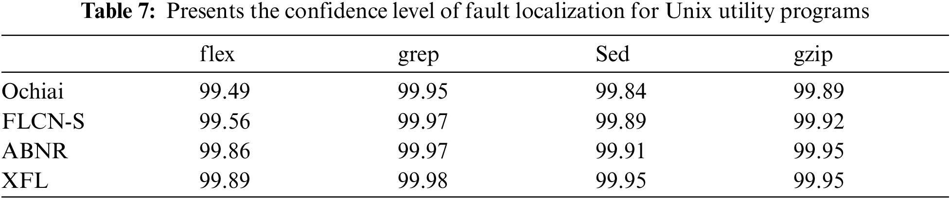
XFL has exhibited a better confidence level for Wilcoxon signed-rank evaluation for determining the correlation among the statements in the software program. In some cases, the performance of the proposed model is slightly better than the ABNR model for subject Unix utility programs. The model is evaluated against the Top-N assessment over the Unix utility program. The observed values are tabulated in concern to the other state-of-art models in Tab. 8.

It can be observed from the experimental values presented in the above table. The proposed XFL model outperforms the other existing model. The model has exhibited an overall performance of 97.4% accuracy, on precisely ranking the vulnerable program statements, which assists in localizing the program's faulty statements.

7  Conclusions

The proposed explainable fault localization model largely focuses on the interpretability and transparency of the decisions made in ranking the statements. Using the suggested paradigm, developers will rapidly and accurately identify the vulnerable statement and assign a rating based on the incorrect statement to all subsequent statements. Compared to other methods of analyzing benchmark subject programs such as the Siemens validation set and Unix utility applications, the suggested method for fault localization demonstrates satisfactory performance. The model is validated using various criteria, including the statements assessed for fault identification, the Wilcoxon signed-rank test, and the Top-N. The findings show that the proposed XFL approach can locate vulnerable statements by analyzing a smaller number of statements with higher confidence. The proposed model is explainable, and the feature weight initialization and the optimization procedures are transparent for analysis. It can be observed from the associated hyperparameters the model has exhibited an optimal performance.

The proposed XFL model is evaluated over the pre-existing dataset for making the statistical analysis more evident. However, the model can be further evaluated against the real-time programs for better evaluation of the real-time performance of the model. Furthermore, to optimize the efforts of training the model, a self-learning model that can dynamically learn from the previous debugging outcomes can be employed for efficient fault localization and to avoid overfitting issues of the model.

Acknowledgement: The author wishes to thank the College of Computer Sciences and Information Technology, King Faisal University, Saudi Arabia, for providing the infrastructure for this study.

Funding Statement: The author did not receive particular funding for this current study. This activity is a component of his academic pursuits.

Conflicts of Interest: The authors declare that they have no conflicts of interest to report regarding the present study.

References

 1.  H. Alaqail and S. Ahmed, “Overview of software testing standard ISO/IEC/IEEE 29119,” IJCSNS International Journal of Computer Science and Network Security, vol. 18, no. 2, pp. 112–116, 2018. [Google Scholar]

 2.  P. Guleria, S. Ahmed, A. Alhumam and P. N. Srinivasu, “Empirical study on classifiers for earlier prediction of COVID-19 infection cure and death rate in the Indian states,” Healthcare, vol. 10, no. 85, pp. 1–32, 2022. [Google Scholar]

 3.  M. -Y. Kim, S. Atakishiyev, H. K. B. Babiker, N. Farruque, R. Goebel et al., “A multi-component framework for the analysis and design of explainable artificial intelligence,” Machine Learning and Knowledge Extraction, vol. 3, pp. 900–921, 2021. [Google Scholar]

 4.  S. Chakraborty, R. Krishna, Y. Ding and B. Ray, “Deep learning based vulnerability detection: Are we there yet?,” arXiv e-prints, 2020. [Google Scholar]

 5.  W. Laura, N. Yannic, V. Thomas, K. Timo and G. Lars, “VUDENC: Vulnerability detection with deep learning on a natural codebase for python,” Information and Software Technology, vol. 144, no. 106809, 2022. [Google Scholar]

 6.  N. Chen, N. Xialihaer, W. Kong and J. Ren, “Research on prediction methods of energy consumption data,” Journal of New Media, vol. 2, no. 3, pp. 99–109, 2020. [Google Scholar]

 7.  W. Sun, X. Chen, X. R. Zhang, G. Z. Dai, P. S. Chang et al., “A multi-feature learning model with enhanced local attention for vehicle re-identification,” Computers, Materials & Continua, vol. 69, no. 3, pp. 3549–3561, 2021. [Google Scholar]

 8.  Z. Chen, W. Ma, W. Lin, L. Chen and B. Xu, “Tracking down dynamic feature code changes against python software evolution,” in 2016 Third Int. Conf. on Trustworthy Systems and Their Applications, Wuhan, China, pp. 54–63, 2016. [Google Scholar]

 9.  A. Alhumam, “Software fault localization through aggregation-based neural ranking for static and dynamic features selection,” Sensors, vol. 21, no. 21, pp. 1–21, 2021. [Google Scholar]

10. X. Mao, Y. Lei, D. Ziying, Q. Yuhua and W. Chengsong, “Slice-based statistical fault localization,” Journal of Systems and Software, vol. 89, pp. 51–62, 2014. [Google Scholar]

11. C. Viji, N. Rajkumar and S. Duraisamy, “Prediction of software fault-prone classes using an unsupervised hybrid SOM algorithm,” Cluster Computing, vol. 22, no. 1, pp. 133–143, 2019. [Google Scholar]

12. K. V. Bakka and A. Deshpande, “Model-based integration and system test automation for visualizing error inclined to an application,” International Journal of Engineering Research, vol. 5, no. 5, pp. 404–407, 2016. [Google Scholar]

13. Y. Pang, X. Xue and A. S. Namin, “Predicting vulnerable software components through n-gram analysis and statistical feature selection,” in 2015 IEEE 14th Int. Conf. on Machine Learning and Applications (ICMLA), Miami, FL, USA, pp. 543–548, 2015. [Google Scholar]

14. K. S. Lwin and B. K. T. Hee, “Predicting SQL injection and cross-site scripting vulnerabilities through mining input sanitization patterns,” Information and Software Technology, vol. 55, no. 10, pp. 1767–1780, 2013. [Google Scholar]

15. H. Turabieh, M. Mafarja and X. Li, “Iterated feature selection algorithms with layered recurrent neural network for software fault prediction,” Expert Systems with Applications, vol. 122, pp. 27–42, 2019. [Google Scholar]

16. A. Balaram and S. Vasundra, “Prediction of software fault-prone classes using ensemble random forest with adaptive synthetic sampling algorithm,” Automated Software Engineering, vol. 29, no. 6, pp. 1–21, 2021. [Google Scholar]

17. N. Sarah, S. Konstantinos and B. Gavin, “On the stability of feature selection algorithms,” The Journal of Machine Learning Research, vol. 18, no. 1, pp. 6345–6398, 2017. [Google Scholar]

18. N. Vafaei, R. A. Ribeiro and L. M. Camarinha-Matos, “Normalization techniques for multi-criteria decision making: Analytical hierarchy process case study,” In: L. M. Camarinha-Matos, A. J. Falcão, N. Vafaei and S. Najdi (Eds.) Technological Innovation for Cyber-Physical Systems (DoCEIS-2016IFIP Advances in Information and Communication Technology, Cham: Springer, vol. 470, pp. 261–269, 2016. [Google Scholar]

19. M. Hutchins, H. Foster, T. Goradia and T. Ostrand, “Experiments on the effectiveness of dataflow and control-flow-based test adequacy criteria,” in Proc. of the 16th Int. Conf. on Software Engineering, Sorrento, Italy, pp. 191–200, 1994. [Google Scholar]

20. Software-Artifact infrastructure repository, [Online]. Available: https://sir.csc.ncsu.edu/php/previewfiles.php (accessed on 28 February 2022). [Google Scholar]

21. A. Zakari, S. Lee and I. Hashem, “A single fault localization technique based on failed test input,” Array, vol. 3, no. 4, pp. 1–13, 2019. [Google Scholar]

22. A. Paul, R. Bandyopadhyay, J. H. Yoon, Z. W. Geem and R. Sarkar, “SinLU: Sinu-sigmoidal linear unit,” Mathematics, vol. 10, no. 337, pp. 1–14, 2022. [Google Scholar]

23. C. -C. Chen, Z. Liu, G. Yang, C. -C. Wu and Q. Ye, “An improved fault diagnosis using 1d-convolutional neural network model,” Electronics, vol. 10, no. 59, pp. 1–19, 2021. [Google Scholar]

24. K. Vijay and D. Bala, “Deep learning,” In: V. Kotu and B. Deshpande (Eds.) Data Science, 2nd Edition, Morgan Kaufmann, Elsevier, Amsterdam, Netherlands, pp. 307–342, 2019. [Google Scholar]

25. A. O. Alzahrani and M. J. F. Alenazi, “Designing a network intrusion detection system based on machine learning for software defined networks,” Future Internet, vol. 13, no. 5, pp. 1–18, 2021. [Google Scholar]

26. P. N. Srinivasu and V. E. Balas, “Self-learning network-based segmentation for real-time brain M. R. images through HARIS,” PeerJ Computer Science, vol. 7, no. e654, 2021. [Google Scholar]

27. P. N. Srinivasu, T. S. Rao and V. E. Balas, “A systematic approach for identifying tumor regions in the human brain through HARIS algorithm,” in Deep Learning Techniques for Biomedical and Health Informatics, Cambridge, MA, USA: Academic Press, 2020. [Google Scholar]

28. P. K. Singh, S. Garg, M. Kaur, M. S. Bajwa and Y. Kumar, “Fault localization in software testing using soft computing approaches,” in Proc. of the 2017 4th Int. Conf. on Signal Processing, Computing and Control (ISPCC), Solan, India, pp. 627–631, 2017. [Google Scholar]

29. L. Zhu, B. Yin and K. Cai, “Software fault localization based on centrality measures,” in Proc. of the 2011 IEEE 35th Annual Computer Software and Applications Conf. Workshops, Munich, Germany, pp. 37–42, 2011. [Google Scholar]

30. H. Tong, S. Wang and G. Li, “Credibility based imbalance boosting method for software defect proneness prediction,” Applied Science, vol. 10, no. 8059, 2020. [Google Scholar]

31. M. Christakis, M. Heizmann, M. N. Mansur, C. Schilling and V. Wüstholz, “Semantic fault localization and suspiciousness ranking,” In: T. Vojnar and L. Zhang (Eds.) Tools and Algorithms for the Construction and Analysis of Systems (TACAS-2019), Prague, Czech Republic, Cham, Switzerland: Springer, vol. 11427, pp. 226–243, 2019. [Google Scholar]

32. R. Hewett, “Program spectra analysis with theory of evidence,” Advances Software Engineering, vol. 2012, no. 642983, 2012. [Google Scholar]

33. S. Pearson, J. Campos, R. Just, G. Fraser, R. Abreu et al., “Evaluating and improving fault localization,” in Proc. of the IEEE/ACM Int. Conf. on Software Engineering, Alamitos, CA, USA, pp. 609–620, 2017. [Google Scholar]

34. W. E. Wong, V. Debroy, Y. Li and R. Gao, “Software fault localization using DStar (D*),” in Proc. of the 2012 IEEE Sixth Int. Conf. on Software Security and Reliability, Washington, DC, USA, pp. 21–30, 2012. [Google Scholar]

35. S. A. Zakari, P. Lee and C. Y. Chong, “Simultaneous localization of software faults based on complex network theory,” IEEE Access, vol. 6, pp. 23990–24002, 2018. [Google Scholar]

This work is licensed under a Creative Commons Attribution 4.0 International License, which permits unrestricted use, distribution, and reproduction in any medium, provided the original work is properly cited.