DOI:10.32604/cmc.2022.029576
| Computers, Materials & Continua DOI:10.32604/cmc.2022.029576 | |
| Article |
Real-time Volume Preserving Constraints for Volumetric Model on GPU
1Department of Software Convergence, Soonchunhyang University, Asan, 31538, Korea
2Department of Computer Science and Engineering, University of Colorado Denver, Denver, 80217, CO, USA
3Department of Computer Software Engineering, Soonchunhyang University, Asan, 31538, Korea
*Corresponding Author: Min Hong. Email: mhong@sch.ac.kr
Received: 07 March 2022; Accepted: 07 April 2022
Abstract: This paper presents a parallel method for simulating real-time 3D deformable objects using the volume preservation mass-spring system method on tetrahedron meshes. In general, the conventional mass-spring system is manipulated as a force-driven method because it is fast, simple to implement, and the parameters can be controlled. However, the springs in traditional mass-spring system can be excessively elongated which cause severe stability and robustness issues that lead to shape restoring, simulation blow-up, and huge volume loss of the deformable object. In addition, traditional method that uses a serial process of the central processing unit (CPU) to solve the system in every frame cannot handle the complex structure of deformable object in real-time. Therefore, the first order implicit constraint enforcement for a mass-spring model is utilized to achieve accurate visual realism of deformable objects with tough constraint error. In this paper, we applied the distance constraint and volume conservation constraints for each tetrahedron element to improve the stability of deformable object simulation using the mass-spring system and behave the same as its real-world counterparts. To reduce the computational complexity while ensuring stable simulation, we applied a method that utilizes OpenGL compute shader, a part of OpenGL Shading Language (GLSL) that executes on the graphic processing unit (GPU) to solve the numerical problems effectively. We applied the proposed methods to experimental volumetric models, and volume percentages of all objects are compared. The average volume percentages of all models during the simulation using the mass-spring system, distance constraint, and the volume constraint method were 68.21%, 89.64%, and 98.70%, respectively. The proposed approaches are successfully applied to improve the stability of mass-spring system and the performance comparison from our experimental tests also shows that the GPU-based method is faster than CPU-based implementation for all cases.
Keywords: Deformable object simulation; mass-spring system; implicit constraint enforcement; volume conservation constraint; GPU parallel computing
Real-time physically-based simulation plays a crucial role in the computer animation industry. Additionally, medical simulation particularly demands animation of the deformable object in real-time and visually realistic animations to represent human organs and soft tissues [1]. Under these circumstances, the applications related to physically-based simulation significantly require both fairly high resolution of 3D mesh and high performance to obtain real-time animation of deformable objects with smooth and responsive interactivity. However, it’s challenging to achieve the main goal of physical simulation with dense mesh structure in real-time due to the large computation. The virtual surgical training system, in particular, requires higher framerates since low framerates can cause glitches and further problems that make users are motion sickness [2]. Therefore, various studies have focused on modeling and simulating deformable objects that can be categorized into continuum mechanics-based techniques, a discrete mass-spring damper technique, and position-based dynamics [3–5].
In continuum mechanics-based techniques, a finite element (FEM) method can deliver a precise result of a deformable object simulation. In addition, FEM is used to represent soft tissues accurately by controlling Young's modulus and Poisson's ratio parameter. However, the computational cost is also high for an interactive simulation, therefore not suitable for real-time deformation. Nevertheless, some researchers have improved FEM techniques to be used in real-time [3]. Mass-spring system (MSS) is simple, easy to implement, and has parameter controllability [4]. The major advantage of MSS is low computation cost. Hence, the result of MSS is inaccurate and unstable, hence potentially producing a huge loss of volume during simulation. The springs in MSS can be nordinately elongated which cause stability and robustness problems. The stability of MSS can be improved by enforcing the geometric constraints on the springs, however it cannot be achieved in real-time performance using only CPU due to the heavy computational cost.
The position-based dynamic (PBD) method is the superior approach that is widely used in various real-time interactive simulations. Unlike FEM and MSS, it determines the projecting position directly to satisfy the existing constraints in the system and omit the velocity layer [5]. PBD is a fast, stable, and effective method however, its numerical result is not accurate compared to FEM and MSS.
Previously, various studies were focusing on the development of high-performance physics simulators for virtual reality (VR) and augmented reality (AR) using graphic processing units (GPU) [6]. Generally, GPUs are utilized mainly for image and animation rendering purposes, however, they are also utilized for general computing. Compared to the traditional approach that implements on the central processing unit (CPU), the GPU-based approach is extremely fast since the direct access to the GPU buffer is more effective than streaming data from the CPU to the GPU buffer [7]. Moreover, GPU-based approaches utilize parallel processing units that processes on muti-cores and thousands of threads at once. Under these circumstances, research on 3D interaction simulation frameworks for VR/AR using the GPU method has been developed to achieve real-time performance under large calculations [8]. In addition, well-known general-purpose computing on the graphics processing unit (GPGPU), compute unified device architecture (CUDA) and Open Computing Language (OpenCL) are normally used as a GPGPU library for any GPU-based approaches [9]. However, it required additional setup and configuration for it to support the graphic library that is not suitable for lightweight applications [10].
Therefore, in this study, we proposed methods for deformable object simulation that use a 3D volumetric model or tetrahedron model to represent the 3D object. The proposed method utilizes parallel processing by using compute shader as GPGPU that existed on OpenGL Shading Language (GLSL). The specific contributions of this paper are:
• The stability of deformable object simulation using the mass-spring system is improved by enforcing the distance constraint to the spring structure and enforcing the volume preservation constraint as maintenance of the local volume during simulation.
• The numerical problem of the constraints system is solved by the parallel method in order to accelerate the performance using compute shader that executes on GPU.
The rest of the paper is structured as follows. Section 2 gives an overview of the previous studies on deformable object simulation. Section 3 presents the proposed method for implementing a mass-spring system and first-order implicit constraint enforcement method based on process distribution on compute shader for simulating object deformation. The data structure for GPU buffer to represent the tetrahedron model for modeling and rendering is also described. Section 4 provides the performance comparison of each method in various 3D objects. To compare the efficiency of each method for deformable object simulation, the overall volume of the 3D object is computed for comparing under the free-fall case. We also compared the performance difference between CPU and GPU-based approaches correspondingly. Section 5 concludes the paper.
FEM is widely used in various dynamic simulation applications due to its high precision and high complexity, as more computing resources are available. The first work on the use of FEM on the linear elastic object was presented in [11]. Later on, Bro-Nielsen et al. [12] reduced the complexity of the volumetric model in order to speed up the result, a model he named as fast finite element models (FFE).
Muller et al. [13] simulated deformable objects using a shape matching approach that found the goal position of each point to satisfy the current state corresponding to the initialize state. They only treat one global constraint for the whole deformed object. Later on, they proposed a position-based dynamic (PBD) simulation supported by explicit integration method [5]. Their key idea was to control the simulation through project positions instead of force. Furthermore, the general constraints can be simply defined via constraint function. A Jacobi, and nonlinear Gauss-Seidel solver were used to solve the dynamic equation of the PBD system.
A mass-spring-damper model is made by a number of nodes connected by springs where each node can have more than one spring. Generally, there are three spring types of cloth models, however, it’s not easy to extract all types of springs to represent general deformable object. Therefore, only structural spring is easily extracted for both surface and volumetric models. Cover et al. [14] presented the first real-time model for surgery simulation using the surface mesh mass-spring model. However, the surface-based model was not well preserved to represent volumetric behavior since the interior structure is not defined. Wang et al. [15] proposed a mass-spring model based on shape matching for a mass-spring model that uses only surface mesh. Zhang et al. [16], used a mass-spring system on a volumetric model based on tetrahedron to maintain the volume of the deformable object to construct the soft tissues. Since the mass-spring model is weak in terms of shape restoration, they applied volume conservation constraints on the tetrahedrons that exist in the model. Additionally, they employed the PBD method for volume conservation constraints to characterize the volumetric model.
Provot [17] and Desbrun et al. [18] used constraint projection in mass-spring systems to prevent springs from overstretching. The implicit constraint enforcement scheme, as according to Hong et al. [19], predicts the correct magnitude of the constraint forces by using future time-steps. Different from the method used by Provot [17], this method is not moving the nodes instantly, instead, they used the geometric constraint over the mass-spring model to prevent the excessive stretching of the springs.
Human muscle dynamics have been modeled and simulated using volume preservation. Hong et al. [20] modeled a mass-spring muscle with volume preservation on the surface mesh. Instead of preserving the local volume of tetrahedral mesh, they used global volume preservation to maintain the global volume of closed mesh topology that represents the deformable object. Zang et al. [21] proposed a soft tissue grasping deformation model to simulate the grasping deformation using the optimized backpropagation neural network to obtain the force and displacement of any mesh point on the soft tissue epidermis.
In this section, we present volume conservation techniques for a deformable object that respect the force-driven method in GPU using parallel processing with different aspects and contributions. We modeled deformable objects using the conventional mass-spring system, distance constraint enforcement, and local volume preservation constraint for a mass-spring system that utilizes the Single Instruction Multiple Data (SIMD) architecture of the GPU. Compute shader was used as kernel program on the GPU for task distribution to obtain high performance.
3.1 Volumetric Model for Deformable Object
Due to the low cost of rendering, most computer-aided design (CAD) and modeling software only work with surface mesh that are represented by a closed triangle. Therefore, the simulation of a deformable object using surface mesh seems to be unrealistic due to the missing interior structure of the topological mesh. The object can be squeezed when the large external force is given. Furthermore, the cutting operations on surface mesh potentially restructure the entire mesh. However, an existing study has presented an approach that adds the internal link to a surface mesh [22]. Also, feature selection can be used to evaluate the selected feature set through a classifier to select the appropriate feature in the geometric constraint datasets [23].
In this work, we used a tetrahedron model to represent the deformable object. The tetrahedron model can be created by various programs and software, among these TetGen [24], generates tetrahedral meshes. TetGen generates polyhedral domain triangulations in three dimensions. It creates meshes with well-shaped elements whose sizes are adjusted according to geometric features or sizing functions provided by the user. The standard input file formats only supports .off file, .ply file, .stl file, and .mesh file. To generate a tetrahedron model from a given surface mesh, TetGen uses a Delaunay-based algorithm. They are capable of preserving any complex geometry or topology. TetGen employs a constrained Delaunay refinement algorithm that maintains mesh quality. TetGen’s robustness is improved by the use of advanced computational geometry technologies. TetGen also inserts the new vertices inside the surface mesh and the new tetrahedron mesh itself in case the user wants to scale the resolution of their mesh. Fig. 1 shows an example of the conversion from surface mesh to tetrahedron mesh. The main output file format for tetrahedrons are:
• .node : a list of nodes or vertices of the mesh.
• .face : a list of triangular faces of the mesh.
• .ele : a list of tetrahedrons of the mesh.
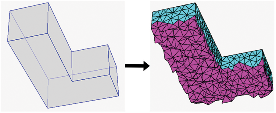
Figure 1: The conversion of a surface mesh to a tetrahedron mesh [22]
Since we used OpenGL as a graphic library for the rendering part, we employed OpenGL Shading Language (GLSL) technology that existed since OpenGL 4.3 was released. In the rendering pipeline, vertex shader, geometry shader, and fragment shader are sequentially executed on the graphic processor to render the images on the display device. Particularly, compute shader is executed outside the rendering pipeline to make the simultaneous thread computes the data in parallel for the non-rendering purpose [25]. Compute shader script is programmed based on C programming syntax. There is the concept of a workgroup to define the compute space for parallel processing.
When a compute operation is invoked, the user specifies the number of workgroups with which it will be executed. These groups’ space is three-dimensional, hence, there are “X”, “Y”, and “Z” groups where any of these can be one, allowing us to create a two-dimensional or one-dimensional computation instead of a three-dimensional one. Each group has its local size with three-dimensional (size can be one to allow two-dimensional or one-dimensional local processing). The specific size is defined in compute shader script, where the number of threads is also define as invocation [26]. This can be used to process image data, linear arrays from a particle system, a cloth model, and other complicated 3D models as well [27].
The shader storage buffer object (SSBO) and image load-store operation are used to output the result data in compute shader since there are no output variables in compute shader. Therefore, we used SSBO for storing data in our proposed algorithm. SSBO stores a massive amount of structured data as a linear array in memory that can be accessed by invocations. SSBO can be adjusted as read-only, write-only, and read-write. Likewise, we use the std430 layout qualifier for initializing compute shader since it does not need data packing before initializing the SSBOs.
3.3 Parallel Mass-Spring System for Tetrahedron Model
In a single tetrahedron, there are four points or nodes, linked by six straight edges and four triangular faces. Fig. 2 illustrates the structure of a single tetrahedron. In the volumetric model represented by a set of tetrahedrons, a pair of two nodes known as spring are extracted from the tetrahedron where each spring must be unique since a single node can be shared with many tetrahedrons. In the general mass-spring-damper model for cloth simulation, the representative types of springs are classified into structural, shear, and flex (bend). Therefore, only structural springs can be easily extracted from the tetrahedron model.
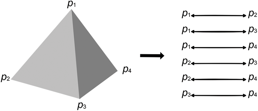
Figure 2: Structure of tetrahedron
Each spring consists of two mass nodes as shown in Fig. 3. Where
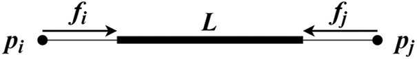
Figure 3: A spring structure in mass-spring damper model
Spring force acting on both nodes can be computed by Hooke’s law as shown in Eq. (1). Where the stiffness and the damping of spring are denoted by
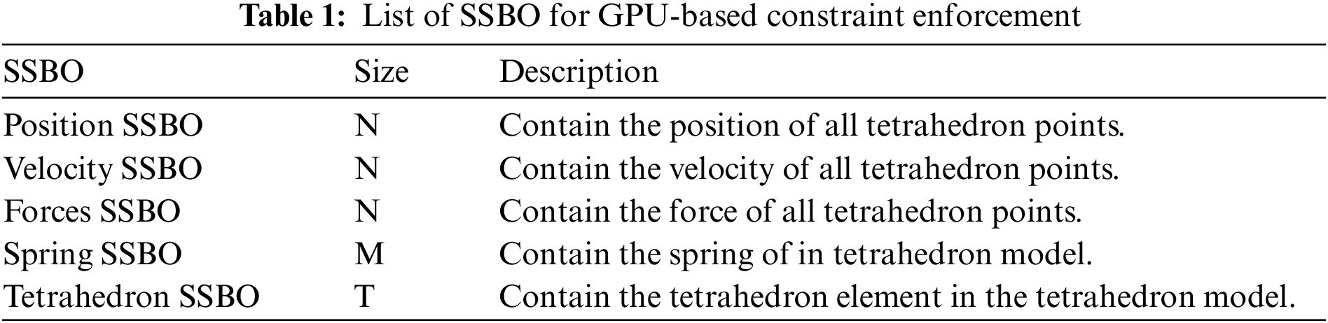
To perform the simulation, there are five SSBOs to store the arrays of data needed to compute in the GPU as shown in Tab. 1. Where N, M, and T are the number of discrete nodes, the number of springs that existed in the tetrahedron model, and the number of tetrahedron elements inside the volumetric model, respectively.
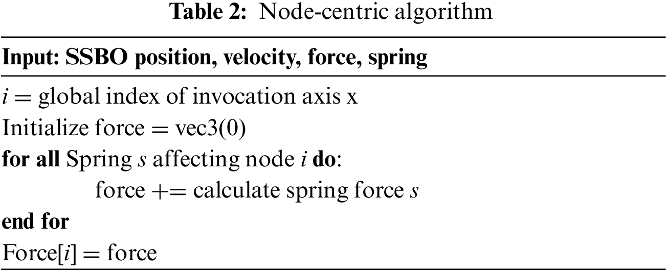
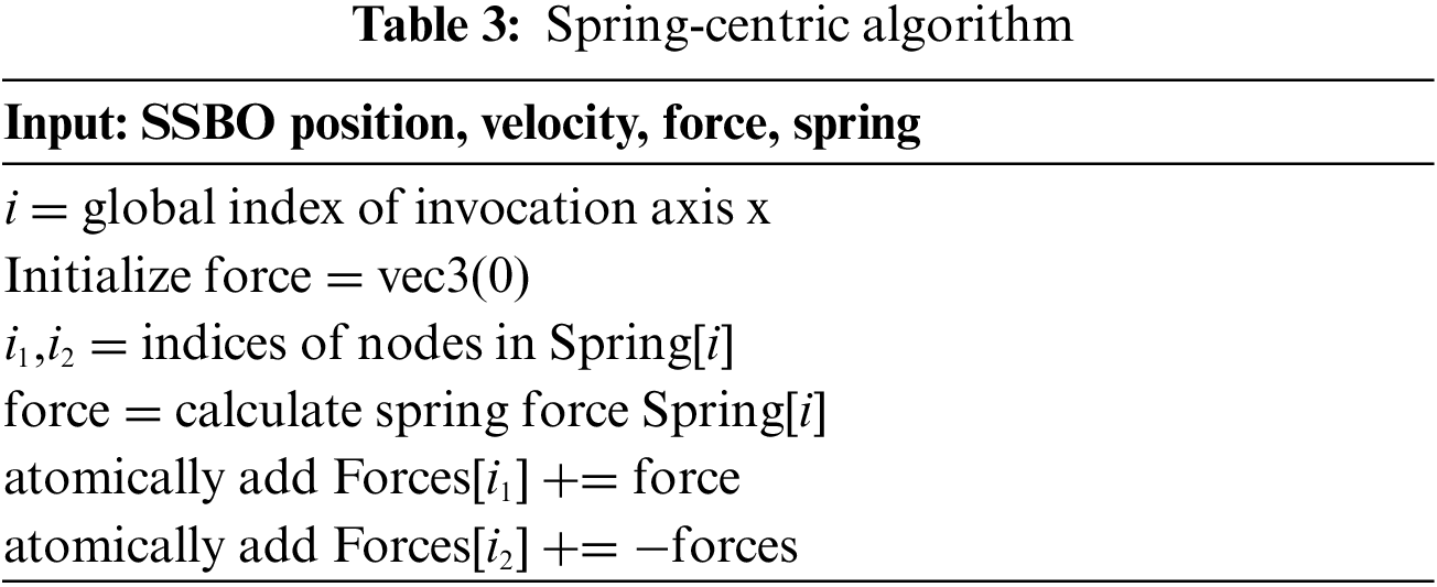
Two compute shaders are required to perform the mass-spring system algorithm in GPU. Springs can be solved in a node-centric or spring-centric manner. In the node-centric approach (See Tab. 2), we assign an invocation or thread per node and loop over all spring affecting it to obtain a good load balancing. After determining the total spring forces, the write operation per node is performed. On the other hand, the spring-centric process a spring for a thread and scatter the force to each affected node. Then a compute shader will invoke two blocks of buffer at the same time causing a problem of data racing on writing data. Therefore, the atomic operation is required to scatter spring force to each affected node (see Tab. 3).
As shown in Eq. (1), the spring equations are linearized and individually solved for each spring, making it is easy to parallelize the algorithm. We then create a one-dimensional compute space for computing force for all nodes (see Section 3.2). Fig. 4 illustrates the compute space for compute forces where
Identically, to determine the new position and velocity of all nodes, we follow Eqs. (2) and (3). The compute space for computing the new position every timeframe of simulation is demonstrated in Fig. 5, where

Figure 4: Compute space for GPU-based mass-spring system using the spring-centric scheme

Figure 5: Compute space for GPU-based mass-spring system using the node-centric scheme
3.4 Parallel Implicit Constraint Enforcement Scheme
The formula of constraint using Lagrange multipliers results in a mixed system of ordinary differential equations (ODE) and algebraic equations. Using 3n generalized coordinate, we obtain Eq. (4), where n denotes the total number of nodes.
The vector of constraint
The partial differentiation on this constraint concerning subscript q obtains a Jacobian matrix
We also applied the local volume constraint over the tetrahedron model. As shown in Fig. 2, a tetrahedron is made by four nodes (
Same as distance constraint, the partial differentiation on volume constraint, we obtain a Jacobian matrix
In an implicit first-order constraint enforcement scheme, the relation between Lagrange multiplier and constraint force is written as follows:
where M is a 3n × 3n diagonal mass matrix,
The implicit constraint enforcement scheme has to solve the problem
The constraint function of the next time is treated implicitly and can be written as
We can eliminate the implicit generalized coordinates
Eq. (17) is simply the linear equation and can be expressed by
In previous work, we applied implicit constraint enforcement for real-time cloth simulation. The parallel method of conjugate gradient solver was used to solve the Eq. (17). However, the performance is poor compared to the conventional mass-spring system since the operation of the sparse matrix becomes a bottleneck [28]. A similar approach has been applied to solve the PBD constraint, where the non-linear Gauss-Seidel solver is used to solve each constraint equation separately, since each constraint has a single scalar value to satisfy the constraints. Each constraint is linearized individually, the solver is more stable than a global approach where the linearization is kept constant throughout the global solution.
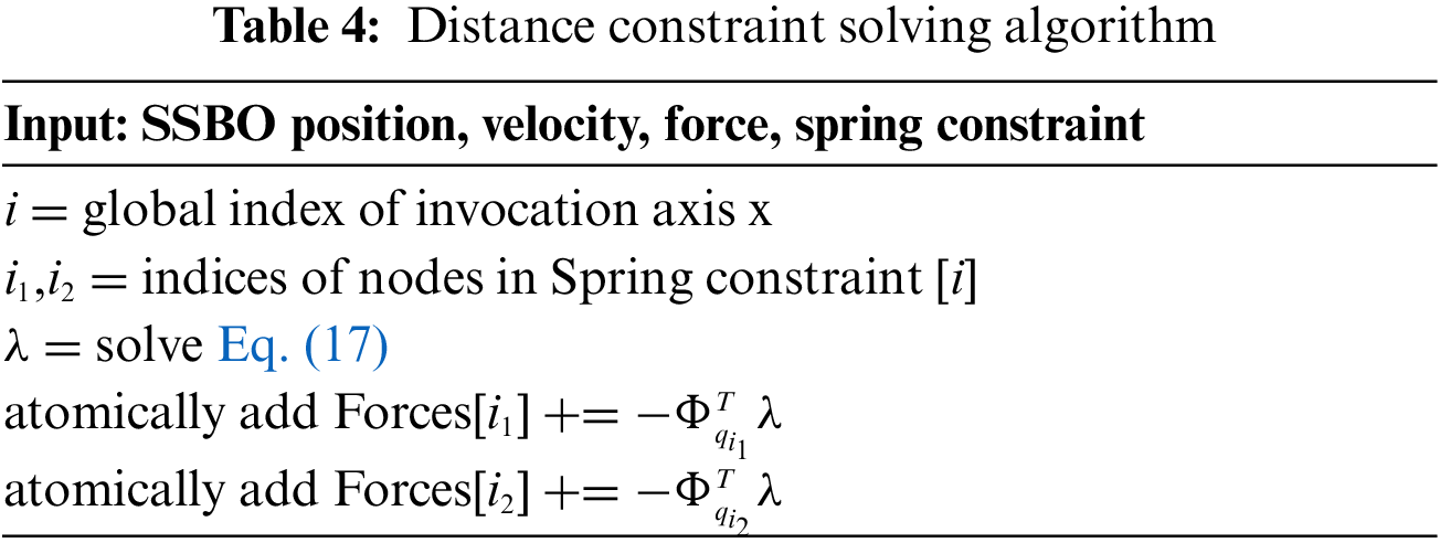
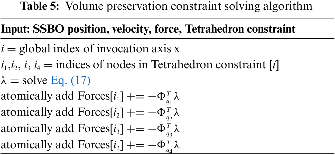
Therefore, we linearized the constraint equation and solved it individually to find each Lagrange multiplier. Then, Eq. (17) seizes from being a linear solving algorithm as the system matrix and right-hand side are scalar values. For distance constraint, we still required two compute shaders for calculating the constraint force and finding the new velocity and position. Tab. 4 shows the algorithm for calculating constraint force using distance constraint. Identically, the implicit constraint enforcement for volume preservation constraint linearized the tetrahedron volume constraint separately. Tab. 5 demonstrated the algorithm for calculating constraint force using volume constraint.
The compute space (see Section 3.2) for distance constraint solving is the same as spring force solving using spring-centric. Fig. 6 demonstrates the compute space for volume constraint solving, where

Figure 6: Compute space for GPU-based volume constraint solving scheme
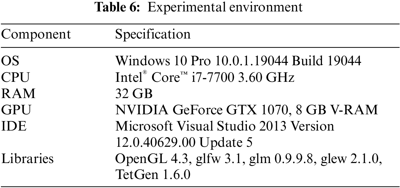
We implemented our proposed method to evaluate the efficiency of volume preservation. Experiments were conducted for the CPU-based and GPU-based approaches to compare the performance that measure in frame per second (FPS). Tab. 6 shows the specifications with which our experiment was conducted on:
We used Stanford’s 3D model made by 3D scanning and available on the Stanford repository [29]. The model data are stored in PLY file format. Therefore, we converted the surface model to the volumetric model using TetGen. Fig. 7 shows a 3D model representing the deformable object.

Figure 7: Volumetric model use in this simulation for performance comparison
To compare the simulation's performance, the vertical synchronization (VSync) is turned off. The maximum number of local sizes for our hardware is 1,536. Alternatively, we found the optimal number to define the local size for general cases of deformable object simulation. The local size of a compute shader for our proposed approach utilized only 1,024 invocations per workgroup. Fig. 8 shows the performance comparison between CPU-based implementation and GPU-based based implement methods.

Figure 8: Performance comparison of deformable object simulation using CPU-based and GPU-based approaches
In the naïve method using CPU-based, the mass-spring method is fast and achieves real-time simulation for all cases compared to other methods. The mass-spring method achieved 32 fps for the largest model (Asian dragon). However, only the Armadillo model could achieve real-time performance for distance constraint and volume preservation constraint methods. A deformable object simulation using our proposed method implemented on GPU achieved real-time performance for all the cases. Although the usage of atomic operation in GPU processing is commonly less efficient, the result showed that the mass-spring system that uses spring-centric is faster than the mass-spring system that uses the node-centric method. This is because the dense connectivity of the springs in the model leads to unbalancing of the amount of process per compute shader program. Also, our GPU hardware is more suitable for this kind of problem, making the spring-centric is faster than the node-centric approach.
As shown in the performance comparison, the mass-spring system is fast but problematic. The simulation using 82k vertices and 93k triangles model still obtain real-time performance with 154 fps using the mass-spring system, 149 fps for distance constraint, and 150 fps for volume preservation constraint method. Fig. 9 shows the minimum volume percentage for all experimental models in a free fall with a simple flat surface as a collider. For the comparison, we used three methods; mass-spring system, constraint enforcement with distance constraint, and constraint enforcement with volume preservation constraint under 400 frames of the simulation. To perform the simulation with stable behavior, we set the timestep to 0.001, and used 10 iterations per frame. The spring stiffness
For the dragon model, the conventional mass-spring system, the minimum volume preservation was 0.04% of the total volume. On the other hand, the volume preservation using distance constraint on mass-spring model obtain a minimum volume of 71.04%. The volume preservation on the mass-spring model well preserves the dragon model with the minimum loss of 92.54% of total volume. The minimum percentage of volume preservation of an Asian dragon model using mass-spring, distance constraint, and volume constraint were 0.01%, 40.2%, and 86.62%, respectively.

Figure 9: Minimum percentage of volume preservation for the three methods
Fig. 10 shows the average volume percentage for all experimental models using the mass-spring system, distance constraint, and volume constraint. The average volume percentage was at least 58.6% for the mass-spring system approach and 77.89% for the distance constraint method. The proposed volume constraint obtained an average of 95.09% for the largest volumetric model. Therefore, the average volume percentage of all models during the simulation using the mass-spring system, distance constraint, and the volume constraint method were 68.21%, 89.64%, and 98.70%, respectively. These show that the mass-spring system is not well preserved and is poor in terms of shape restoration while the distance constraint approach obtains better results. Overall, the proposed approach of volume preservation constraint deliver sophisticated result with significant improvement for the percentage of the deformable object’s volume. The volume preservation constraint approaches are successfully applied to improved the stability of mass-spring system for the large and complex model of the deformable object. Fig. 11 shows the snapshots of the simulation we conducted.

Figure 10: Average percentage of volume preservation for the three methods

Figure 11: (a) Snapshots of the simulation using the Stanford armadillo model. (b) Snapshots of the simulation using the Stanford dragon model
We proposed a method to design and implement the simulation of volumetric objects based on the mass-spring system and constraint enforcement method that applied CPU-based and GPU-based methods. The mass-spring system required a suitable parameter to achieve stable and effective behavior. Therefore, a constraint-based method is stable and well preserves the volume of the 3D objects compared to a mass-spring method. The average volume percentage of all models during the simulation using the mass-spring system, distance constraint, and the volume constraint method were 68.21%, 89.64%, and 98.70%, respectively. The performance result also proves that the constraint-based approaches are not as fast as the mass-spring system. However, the distance constraint on the mass-spring model to preserve the local element (tetrahedron) is more efficient than the conventional mass-spring system. Our local volume preservation constraint on the mass-spring model is the more efficient and well-preserved global volume of a volumetric object compared to the other two methods. Hence, the volume preservation constraint provides good shape restoration ability for the incompressible soft-body object. The usage of compute shader, executed in GPU processing, made our proposed approaches faster than the traditional CPU-based method. Furthermore, the simulation using 82k vertices and 93k triangles model produced real-time performance with 154 fps using the mass-spring system, 149 fps for distance constraint, and 150 fps for volume preservation constraint method.
However, the limitation of our deformable object simulation is that it requires the pre-processing stage to construct the tetrahedron model using the TetGen library from the given surface model. On the other hand, the compute shader is not supported with float-type data for an atomic operation, for this reason, we utilize the NVIDIA extension, which provides the additional extension library for floating-point operation. Also, our proposed approach might not run in different environments besides the NVIDIA GPU model, which is an open problem for a multi-GPU-based approach. Another limitation is that we only defined the one-dimensional workgroup and the number of invocations per workgroup as 1024. However, the adaptive size for local workgroup remains a question and an important topic for future research. On the other hand, we did not apply self-collision detection and response while it is an important part of physically-based simulation.
In future work, we will apply global volume preservation constraints on the deformable object to speed up the performance, since the volume of the surface model can be simply calculated using the divergence theorem. We will also focus on the complex biological characteristics of the soft tissue model. Besides that, we will focus on self-collision detection and the response part without a significant computational burden. In addition, the human organs model can be represented using our proposed approach and interact in real-time which is beneficial for virtual surgery using AR/VR devices.
Funding Statement: This work was supported by the Basic Science Research Program through the National Research Foundation of Korea (NRF-2019R1F1A1062752), funded by the Ministry of Education; was funded by BK21 FOUR (Fostering Outstanding Universities for Research) (No.: 5199990914048); and was also supported by the Soonchunhyang University Research Fund.
Conflicts of Interest: The authors declare that they have no conflicts of interest to report regarding the present study.
1. W. Shi, P. X. Liu and M. Zheng, “Cutting procedures with improved visual effects and haptic interaction for surgical simulation systems,” Computer Methods and Programs in Biomedicine, vol. 184, no. 4, pp. 105270, 2020. [Google Scholar]
2. Y. Ryu and E. Ryu, “Overview of motion-to-photon latency reduction for mitigating VR sickness,” KSII Transactions on Internet and Information Systems, vol. 15, no. 7, pp. 2531–2546, 2021. [Google Scholar]
3. A. Lamecki, A. Dziekonski, L. Balewski, G. Fotyga and M. Mrozowski, “GPU-accelerated 3D mesh deformation for optimization based on the finite element method,” Radioengineering, vol. 26, no. 4, pp. 924–929, 2017. [Google Scholar]
4. K. Golec, “Hybrid 3D mass spring system for soft tissue simulation,” Ph.D. dissertation. University of Lyon, France, 2018. [Google Scholar]
5. M. Müller, B. Heidelberger, M. Hennix and J. Ratcliff, “Position based dynamics,” Journal of Visual Communication and Image Representation, vol. 18, no. 2, pp. 109–118, 2007. [Google Scholar]
6. H. Hyder, G. Baloch, K. Saad, N. Shaikh, A. B. Buriro et al., “Particle physics simulator for scientific education using augmented reality,” International Journal of Advanced Computer Science and Applications, vol. 12, no. 2, pp. 671–681, 2021. [Google Scholar]
7. W. Shin, K. H. Yoo and N. Baek, “Large-scale data computing performance comparisons on SYCL heterogeneous parallel processing layer implementations,” Applied Sciences, vol. 10, no. 5, pp. 1656, 2020. [Google Scholar]
8. H. Va, M. H. Choi and M. Hong, “Real-time cloth simulation using compute shader in Unity3D for AR/VR contents,” Applied Sciences, vol. 11, no. 17, pp. 8255, 2021. [Google Scholar]
9. Y. Yamato, “Study and evaluation of improved automatic GPU offloading method,” International Journal of Parallel, Emergent and Distributed Systems, vol. 36, no. 6, pp. 594–608, 2021. [Google Scholar]
10. H. Va, D. Lee and M. Hong, “Parallel algorithm of conjugate gradient solver using OpenGL compute shader,” Journal of the Korea Society of Computer and Information, vol. 26, no. 1, pp. 1–9, 2021. [Google Scholar]
11. M. Bro-Nielsen and S. Cotin, “Soft tissue modeling in surgery simulation for prediction of results of craniofacial operations & steps toward virtual reality training systems,” in Proc. 3rd Int. Workshop Rapid Prototyping in Medicine & Computer-Assisted Surgery, Erlangen, Germany, pp. 35, 1995. [Google Scholar]
12. M. Bro-Nielsen and S. Cotin, “Real-time volumetric deformable models for surgery simulation using finite elements and condensation,” in Computer Graphics Forum. Edinburgh, UK: Blackwell Science Ltd, pp. 57–66, 1996. [Google Scholar]
13. M. Muller, B. Heidelberger, M. Tescher and M. Gross, “Meshless deformations based on shape matching,” ACM Transactions on Graphics (TOG), vol. 24, no. 3, pp. 471–478, 2005. [Google Scholar]
14. S. A. Cover, N. F. Ezquerra, J. F. O’Brien, R. Rowe, T. Gadacz et al., “Interactively deformable models for surgery simulation,” IEEE Comput. Graphics Applicat. Mag, vol. 13, no. 6, pp. 68–75, 1993. [Google Scholar]
15. Y. Wang, Y. Xiong, K. Xu, K. Tan and G. Guo, “A mass-spring model for surface mesh deformation based on shape matching,” in Proc. of the 4th Int. Conf. on Computer Graphics and Interactive Techniques in Australasia and Southeast Asia 2006, Kuala Lumpur, Malaysia, pp. 375–380, 2006. [Google Scholar]
16. X. Zhang, H. Wu, W. Sun and C. Yuan, “An optimized mass-spring model with shape restoration ability based on volume conservation,” KSII Transactions on Internet and Information Systems, vol. 14, no. 4, pp. 1738–1756, 2020. [Google Scholar]
17. X. Provot, “Deformation constraints in a mass-spring model to describe rigid cloth behavior,” in Graphics Interface Canadian Human-Computer Communications Society. Quebec City, QC, Canada, 147–154, 1995. [Google Scholar]
18. M. Desbrun, P. Schröder and A. Barr, “Interactive animation of structured deformable objects,” in Proc. of Graphics Interface '99, Kingston, Ontario, Canada, pp. 2–4, 1999. [Google Scholar]
19. M. Hong, M. H. Choi, S. Jung, S. Welch and J. Trapp, “Effective constrained dynamic simulation using implicit constraint enforcement,” Computational Science—ICCS 2006. Lecture Notes in Computer Science, vol. 3991, pp. 490–497, 2006. [Google Scholar]
20. M. Hong, S. Jung, M. H. Choi and S. W. J. Welch, “Fast volume preservation for a mass-spring system,” IEEE Computer Graphics and Applications, vol. 26, no. 5, pp. 83–91, 2006. [Google Scholar]
21. X. R. Zhang, X. Sun, W. Sun, T. Xu and P. P. Wang, “Deformation expression of soft tissue based on BP neural network,” Intelligent Automation & Soft Computing, vol. 32, no. 2, pp. 1041–1053, 2022. [Google Scholar]
22. D. Lee, T. W. Kim, Y. J. Choi and M. Hong, “Volumetric object modeling using internal shape preserving constraint in Unity 3D,” Intelligent Automation & Soft Computing, vol. 32, no. 3, pp. 1541–1556, 2021. [Google Scholar]
23. M. Yang and J. Yang, “Feature selection based on distance measurement,” Journal of New Media, vol. 3, no. 1, pp. 19–27, 2021. [Google Scholar]
24. H. Si, “TetGen, a Delaunay-based quality tetrahedral mesh generator,” ACM Transactions on Mathematical Software (TOMS), vol. 41, no. 2, pp. 1–36, 2015. [Google Scholar]
25. J. Kessenich, D. Baldwin and R. Rost, “The OpenGL shading language,” 2013. [Online]. Available: https://www.khronos.org/registry/OpenGL/specs/gl/GLSLangSpec.4.30.pdf. [Google Scholar]
26. D. Shreiner, G. Sellers, J. Kessenich and B. Licea-Kane, Compute Shader. In: OpenGL Programming Guide: The Official Guide to Learning OpenGL, Version 4.3, 8th ed., Boston, MA, USA: Addison-Wesley, 2013. [Online]. Available at: https://www.cs.utexas.edu/users/fussell/courses/cs354/handouts/Addison.Wesley.OpenGL.Programming.Guide.8th.Edition.Mar.2013.ISBN.0321773039.pdf. [Google Scholar]
27. H. Va, M. H. Choi and M. Hong, “Parallel cloth simulation using OpenGL shading language,” Computer Systems Science and Engineering, vol. 41, no. 2, pp. 427–443, 2022. [Google Scholar]
28. W. Lee, M. Kim and J. Park, “Speed-up of the matrix computation on the ridge regression,” KSII Transactions on Internet and Information Systems, vol. 15, no. 10, pp. 3482–3497, 2021. [Google Scholar]
29. M. Levoy, J. Gerth, B. Curless and K. Pull, “The stanford 3D scanning repository,” 2004. [Online]. Available: http://www-graphics.stanford.edu/data/3Dscanrep/. [Google Scholar]
 | This work is licensed under a Creative Commons Attribution 4.0 International License, which permits unrestricted use, distribution, and reproduction in any medium, provided the original work is properly cited. |