Computers, Materials & Continua DOI:10.32604/cmc.2022.025751
Article

Linear Active Disturbance Rejection Control with a Fractional-Order Integral Action

Maâmar Bettayeb1,3, Rachid Mansouri2,*, Ubaid M. Al-Saggaf3,4, Abdulrahman U. Alsaggaf3,4 and Mohammed Moinuddin3,4

1Electrical Engineering Department, University of Sharjah, United Arab Emirates
2L2CSP Laboratory, University Mouloud Mammeri of Tizi-Ouzou, Algeria
3Center of Excellence in Intelligent Engineering Systems (CEIES), King Abdulaziz University, Jeddah, Saudi Arabia
4Electricaland Computer Engineering Department, King Abdulaziz University, Jeddah, Saudi Arabia
*Corresponding Author: Rachid Mansouri. Email: rachid.mansouri@ummto.dz
Received: 03 December 2021; Accepted: 13 April 2022

Abstract: Linear active disturbance rejection control (LADRC) is a powerful control structure thanks to its performance in uncertainties, internal and external disturbances estimation and cancelation. An extended state observer (ESO) based controller is the key to the LADRC method. In this article, the LADRC scheme combined with a fractional-order integral action (FOI-LADRC) is proposed to improve the robustness of the standard LADRC. Using the robust closed-loop Bode’s ideal transfer function (BITF), an appropriate pole placement method is proposed to design the set-point tracking controller of the FOI-LADRC scheme. Numerical simulations and experimental results on a cart-pendulum system will illustrate the effectiveness of the proposed FOI-LADRC scheme for the disturbance rejection, the set-point tracking and the improved robustness. To illustrate the LADRC control schemes and to verify the performance of the proposed FOI-LADRC, compared to the standard LADRC and IOI-LADRC structures, two tests will be carried out. First, simulation tests on an academic example will be presented to show the effect of the different parameters of the control law on the performance of the closed-loop system. Then, these three control structures are implemented on an experimental test bench, the cart-pendulum system, to show their efficiency and to show the superiority of the proposed method compared to the two other structures.

Keywords: Fractional calculus; active disturbance rejection control; pole placement; cart-pendulum system; robust control

1  Introduction

Nowadays, industrial systems are becoming more and more complex, making their analysis and control very difficult. Several robust control systems design methods have been developed recently. Nevertheless, in addition to non-linear behavior, uncertainty is unavoidable during the modeling of these physical systems. Uncertainties can be internal (unknown parameters or unmodelled dynamics) and external (disturbances). Recently, research on the control of uncertain systems has shown the use of several methods. These include: (1) the sliding mode control method, which is mainly used for linear or non-linear systems affected by external disturbances [1]; (2) methods using the linear matrix inequalities, which apply to interval systems with parameters uncertainties [2,3]; and (3) methods using data driven control, based on ultra-local models and on online parameter identification [4,5]. In addition to these methods, another effective scheme is proposed by Han [6,7], where the internal and the external disturbances are considered as a generalized disturbance. Based on an Extended State Observer (ESO), this generalized disruption is estimated and canceled by a judicious feedback loop. Simulation results as well as experimental results have been reported in several examples (see for example [8–10]).

The linear active disturbance rejection control (LADRC) with an integral action (IOI-LADRC) is presented in [11]. This control structure is interesting insofar as it solves the set-point tracking problem as well as the disturbance rejection in a better way than the standard scheme, especially when the external disturbances are variable [11]. The generalization of this structure to the fractional-order case consists in replacing the integer integration action by a non-integer order one. In this case, the challenge is to propose a design method to calculate the parameters of the obtained fractional-order control law, notably the non-integer order introduced by the fractional-order operator. In the state space representation, the solution that is often used is the pole placement method. Nevertheless, this solution is not obvious in the fractional-order case because of the non-integer order [12,13].

One solution is to use the so called “augmented model” corresponding to the fractional-order model [14–17]. In this solution, the non-integer order is not designed in accordance with the closed-loop reference model; it is rather chosen, and it must be rational. Afterwards, using a suitable change of variable, the characteristic polynomial of the augmented model can be reduced to an integer polynomial. An appropriate pole placement is then used to design the parameters of the control law. This method has two major disadvantages. On the one hand, the non-integer order of the control law is not designed in relation to the closed-loop reference behavior, and it must be rational. On the other hand, the degree of the integer-order of the characteristic polynomial corresponding to the augmented model is very high, which requires the designer to choose a large number of poles; while the fractional-order model does not require that number [18].

Another solution is to find a design method that makes it possible to calculate both the non-integer order introduced by the fractional-order integrator and the parameters of the control law, based on the desired closed-loop performance. This is precisely what we present in this paper: based on the Bode's ideal transfer function (BITF) [19,20], the proposed method makes it possible to impose the iso-damping property to the closed-loop response, so as to make the control law more robust.

The main contributions of this paper are:

•   To control systems with high relative degree using fractional-order controllers and to impose the flatness of the phase margin, a new reference model using the BITF is proposed. This makes it possible to impose, in the closed-loop response, the iso-damping property.

•   A control structure, the LADRC control scheme associated with a fractional-order integral action inserted in the set-point tracking loop is proposed.

•   Based on the BITF, a new design method of the set-point tracking controller is the main theoretical contribution.

•   Numerical simulations are presented in order to validate these theoretical results, in particular the robustness of the control structure with respect to the set-point tracking controller gain variations.

•   The proposed LADRC with a fractional-order integral action control structure is also implemented on an experimental testbed consisting of a pendulum cart system. We have shown that this structure can be implemented without modeling the system and that it has made it possible to improve the robustness of the LADRC control scheme compared to the exiting schemes in the literature.

2  Preliminary

2.1 LADRC: Standard Formulation

In the standard formulation of the LADRC approach, for a linear integer-order system, it is not necessary to have the complete model of the system to be controlled. The information on which this method is based is the relative degree and the high frequency gain of the model [7,8,21]. The controlled system is modeled by:

{y(n)(t)=b0u(t)+f(t)f(t)=f(t,y(i),u(i),d(i),d)+(b−b0)u(t)(1)

where y(n)(t) is the nth derivative of y(t), u(t) and y(t) are, respectively, the input and the output, d(t) is the external disturbance, n is the relative degree, b0 is the estimate value of the gain b and f(t) is the generalized disturbance. y(i), u(i) and d(i) are the nth derivatives of u(t), y(t) and d(t), respectively.

In the LADRC approach, the key is to estimate the unknown generalized disturbance f(t) using an ESO. Assume that f(t) is differentiable; consider the extended state space model corresponding to Eq. (1).

System:{x˙=Ax+Bu+Ehy=Cx(2)

where xs=[yy˙⋯y(n−1)]T, x=[xsf], h=f˙

A=[010⋯0001⋯0⋮00⋮00⋮00⋱⋯⋯⋮10],B=[00⋮b00],E=[00⋮01],C=[10000]

The structure of the full ESO is given by

ESO:{z˙=Az+Bu+L(y−y0)y0=Cz(3)

where zs is the estimate of xs, zn+1 the estimate of f(t), and L the gain vector of the observer.

L=[β1β2⋯βnβn+1](4)

The parameters βi (i=1,⋯,n+1) are determined so that (A−LC) is asymptotically stable. Il this case, variables zi(t) (i=1,⋯,n) approximate the output y(t) and its (n−1) derivatives, and zn+1(t) approximates the unknown generalized disturbance f(t). To reject the estimated disturbance, the control law is chosen as:

u(t)=1b0[u0(t)−zn+1(t)](5)

If the estimated error is ignored (we assume that (zn+1(t)=f(t)), then Eq. (1) is reduced to n cascaded integer-order integral operators.

y(n)(t)=u0(t)(6)

In the standard form, a state feedback is used to solve the set-point tracking problem. So, the control law u(t) is given by: [7]

u(t)=K0(r^(t)−z(t))(7)

where r^(t) is the new reference signal obtained from the reference signal r(t) and its (n−1) derivatives.

r^(t)=[r(t)r˙(t)⋯r(n−1)(t)0]T(8)

and

K0=1b0[k1k2⋯kn1](9)

The structure of the standard LADRC is shown in Fig. 1. It has two gain vectors to design: the gain L of the ESO and the gain K0 of the controller. To do this, the method proposed in [22] is often used, which comes down to two parameters: the controller bandwidth ωc and the observer bandwidth ω0.

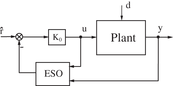
Figure 1: Standard LADRC scheme

2.2 LADRC with Integer Integral Action

To improve the performance of the standard LADRC for uncertain systems, in particular with respect to external disturbances, a control scheme associating an LADRC with an integer-order integral action, (IOI-LADRC) is proposed in [11]. The new control scheme is shown in Fig. 2.

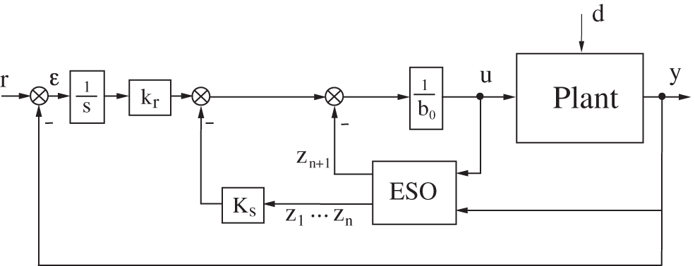
Figure 2: Control structure of LADRC with integer integral action

An additional state is introduced: the integral of the set-point tracking error is given by:

xr(t)=∫0t(r(τ)−y(τ))dτ(10)

where r(t) is the reference signal and y(t) is the output. The new state xr(t) denotes the tracking error, at it will be included in the control law. In this case, the control signal of Eq. (7) becomes

u(t)=1b0(krxr(t)−Kszs(t)−zn+1(t))(11)

where: Ks=[ks1ks2⋯ksn] and kr are the feedback gains of the observed variable and the added integration state, respectively. The pole placement method can be used to design these parameters. Assuming that the observer is well designed (the original plant (1) is transformed to cascaded integrators (6)), the transfer function between r(s) and y(s) is:

Gyr(s)=krsn+1+ksnsn+ksn−1sn−1+…+ks1s+kr(12)

In this case too, the solution suggested in [20] is used. So, (12) should be

Gyr(s)=(krs+ωc)n+1(13)

Thus, the controller parameters are tuned as [11].

[krks1⋯ksn]=[ωcn+1αn+1ωcnαn⋯ωcα1](14)

αi=(n+1)!i!(n+1−i)!i=1,⋯,n+1

With the integral action added in the feedback loop, the disturbance rejection is improved. In addition, the steady error for changing the disturbance or the reference signal can be eliminated. This feature is not possible with the standard LADRC [11].

2.3 Bode’s Ideal Transfer Function

In the fractional-order controllers design, the new degree of freedom introduced by the controller (the non-integer order) is used, so that at least one characteristic of the closed loop system will depend only on it. In this case, this feature will be insensitive to the changes of the system or controller parameters. To address this issue, one solution is to impose, on the open-loop, a behavior equivalent to that of Bode’s ideal transfer function [18,23–26]. The open-loop transfer function suggested by [19] is:

Gol(s)=1τcsλ+1λ∈R(15)

The gain crossover frequency depends on the times constant τc and the phase, which is an horizontal line, dependsonly on the non-integer order λ. The corresponding closed-loop is then

Gcl(s)=11+τcsλ+1(16)

Its step response for (0<λ<1) which is equivalent to that of a second-order model for a damping ration is (0<ξ<1). However, it exhibits the so-called iso-damping property. In this paper, the adjustable parameters τc and λ of Gcl(s) are used to tune the control law parameters.

When the relative degree of the model is greater than 2, to obtain, in open-loop, a transfer function equal to (12), the set-point tracking controller should be complex. To simplify its design, the transfer function (17) is proposed as the new open-loop reference model:

Gol(s)=1(1+Ts)n−1τcsλ+1(17)

for which it corresponds in closed-loop, the transfer function:

Gcl(s)=11+(1+Ts)n−1τcsλ+1(18)

n is the relative degree and τc and λ are the design parameters of (15). T is an additional time constant which must be chosen as small as possible according to τc so that the dynamics it generates will not modify the dynamics of the BITF imposed by τc and λ.

Fig. 3 shows the Bode diagram of (17) for (n=1,2,3,4) when λ=0.3, τc=0.5 and T=τc/50. Fig. 4 shows the step responses of (18) for three values of τc. These Figures prove that the behavior of the transfer function (13) is very close to that of the BITF (10). Fig. 3, in particular, shows the iso-damping property of the closed-loop step response.

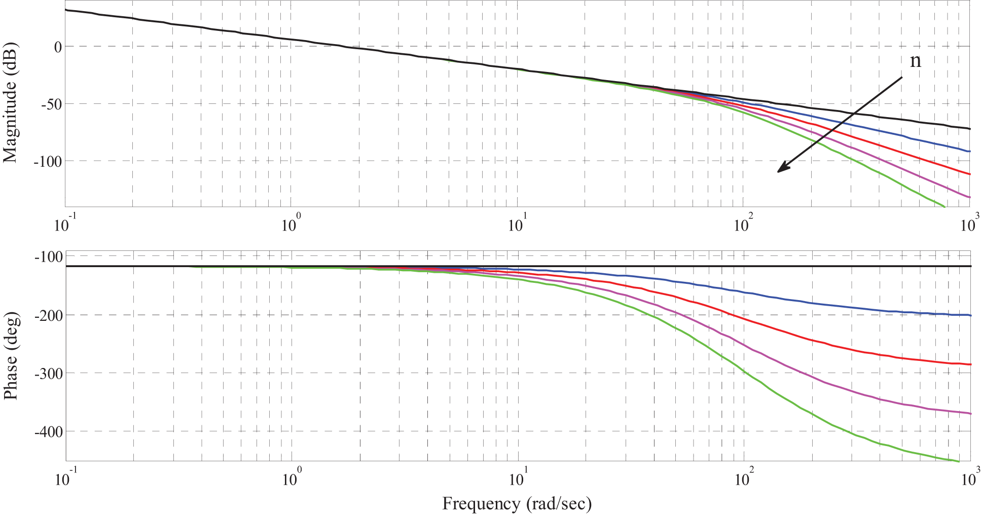
Figure 3: Bode diagram of Gol(s) (17)

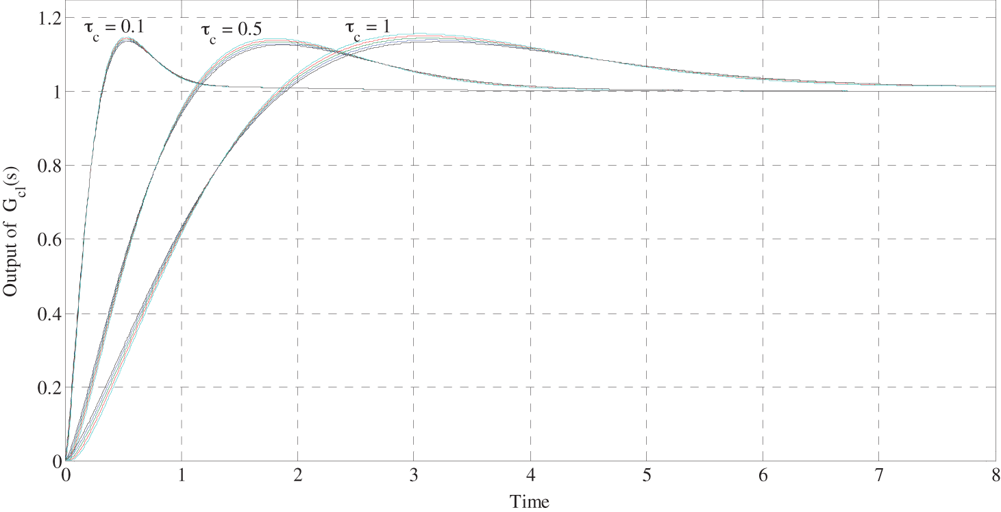
Figure 4: Step response of the close-loop (18) corresponding to Gol(s) (17)

Remark: To link with the standard LADRC, the set-point tracking controller parameter design ωc is replaced by the two parameters τc and λ and ω0 is still used to tune the observer gain. In addition, in order for the observer to correctly estimate the generalized disturbance, the frequency corresponding to the time constant T must be smaller than ω0.

3  LADRC with Fractional-Order Integral Action

The LADRC with a fractional-order integral action (FOI-LADRC) scheme is the same as that of Fig. 2 where the integer-order integral action is replaced by a fractional-order one. The state feedback Ks allows to arbitrary place the n poles of the closed-loop characteristic polynomial. It is associated with the gain kr of the fractional integration to impose to the closed-loop the BITF (18). This makes it possible to increase the robustness of the LADRC structure with respect to the set-point open-loop gain. The ESO is that of Eq. (3).

So, the control signal is given by:

u(t)=1b0[krIα(r(t)−y(t))−Kszs(t)−zn+1(t)](19)

where Iα(.) denotes the fractional-order integral operator [27].

The objective is to propose a method to design the state feedback vector Ks, the coefficient kr and the non-integer order α (0<α<1) of the fractional-order integrator of (19) when the closed-loop reference model is (18).

Theorem 1. Consider the integer-order model (1) representing a stable linear minimum phase system. ESO (3) is used to estimate the generalized disturbance f(t) involved in the model (1). The parameters of the FOI-LADRC (19), which allow to obtain, in closed-loop, the reference model (18) are given by:

α=λ,kr=1Tn−1τc,(20)

and

Ks=[n−1T(n−2)(n−1)2!T2(n−3)(n−2)(n−1)3!T3⋯1Tn−10](21)

λ, τc and T are the parameters of the closed-loop reference model (18) and n is the relative degree of the integer-order model (1).

Proof: Assume that the extended observer is well designed (we assume that zn+1(t)=f(t)). From Fig. 5, the transfer function between ε(s) and y(s) is given by:

y(s)ε(s)=krΔol(s)sα(22)

where

Δol(s)=sn+ks1sn−1+ks2sn−2+…+ksn−1s+ksn(23)

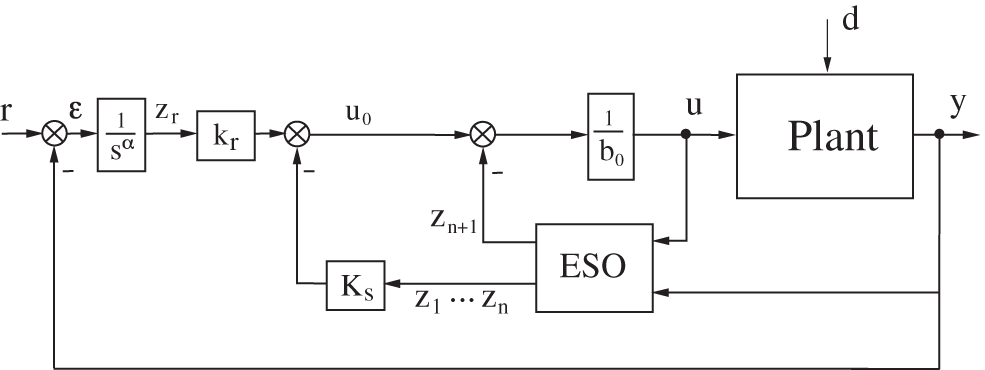
Figure 5: LADRC with a fractional-order integral action

To obtain, in open-loop, the transfer function (17), we must maintain one pole of Δol(s) equal to zero to combine it with that of the fractional-order integrator to obtain the BITF (19). To do this, we put:

ksn=0(24)

In this case, the transfer function (22) becomes, after dividing by ksn−1:

y(s)ε(s)=1ksn−1krΔol(s)sα+1(25)

and Δol(s) becomes a (n−1)th order polynomial. It is given by:

Δol(s)=1ksn−1sn−1+ks1ksn−1sn−2+ks2ksn−1sn−3+…+ksn−2ksn−1s+1(26)

To obtain, in open-loop, a behavior equivalent to that of the BITF, we impose that the imposed transfer function (25) must have the form of the transfer function (17). To do this, we must have:

α=λandksn−1kr=τc(27)

On the other hand, using Newton’s binomial formula, we have:

(1+Ts)n−1=∑k=0n−1(n−1k)(Ts)k(28)

A term-by-term identification of the coefficients of (28) and those of the integer-order denominator of the transfer function (26), leads to:

ks1=n−1T,ks2=(n−2)(n−1)2!T2,ks3=(n−3)(n−2)(n−1)3!T3,…,ksn−2=(n−1)Tn−2,ksn−1=1Tn−1(29)

Substituting the expression of ksn−1 into (27), we obtain:

kr=1Tn−1τc(30)

This completes the proof.

4  Frequency Domain Characteristics Analysis

To analyze the characteristics of the FOI-LADRC in the frequency domain and to avoid complex mathematical expressions, we present, in what follows, the most common case of the second-order FOI-LADRC. In this case, matrices of the ESO (3) are given by:

A=[010001000],B=[0b00],C=[100],L=[3ω03ω02ω03](31)

From the observer state model, it is easy to deduce the transfer functions between the two inputs u(s) and y(s) and the estimated states z2(s) and z3(s) used in the control law. We find:

z2(s)=G1(s)u(s)+G2(s)y(s)(32)

z3(s)=G3(s)u(s)+G4(s)y(s)(33)

where:

G1(s)=b0s(s+β1)Δ(s),G2(s)=s(β2s+β3)Δ(s),G3(s)=β3b0Δ(s),G4(s)=β3s2Δ(s)(34)

and

Δ(s)=(s+ωo)3=s3+3ωos2+3ωo2s+ωo3(35)

Using these equations, the closed-loop control scheme of Fig. 5 becomes that represented by Fig. 6. In order, to calculate the expressions of u(s) according to r(s) and y(s), the block diagram of Fig. 6 is transformed into that of Fig. 7, where:

H(s)=1b01+1b0(ks1G1(s)+G3(s))=Δ(s)b0dH(s)(36)

F(s)=ks1G2(s)+G4(s)=nF(s)Δ(s)(37)

and

dH(s)=s3+(β1+ks1)s2+(β2+β1ks1)snF(s)=(ks1β2+β3)s2+β3ks1s(38)

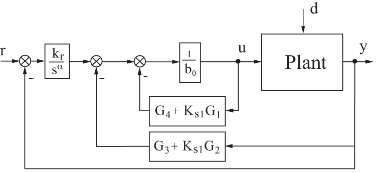
Figure 6: Block diagram of the second order FOI-LADRC

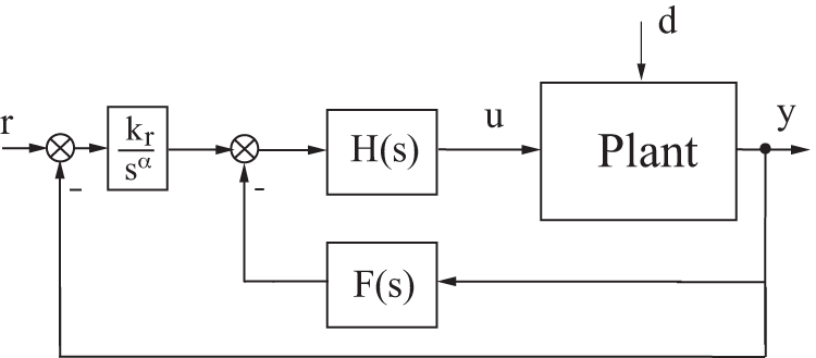
Figure 7: Simplified block diagram of the second order FOI-LADRC

From Fig. 7, we can now deduce the transfer function between r(s) and y(s) and between f(s) and y(s).we get:

u(s)=H(s)(krsα(r(s)−y(s))−F(s)y(s))(39)

Based on Eq. (1) and taking into account the disturbances du(s) on the input and dy(s) on the output, we can write the following equation:

u(s)=s2b0(y(s)+dy(s))−1b0f(s)−du(s)(40)

The equality of Eqs. (39) and (40) leads to:

y(s)=Gry(s)r(s)+Gfy(s)f(s)+Gduy(s)du(s)+Gdyy(s)dy(s)(41)

where

Gry(s)=1sαkrH(s)D(s),Gfy(s)=1b01D(s),Gduy(s)=1D(s),Gdyy(s)=s2b01D(s)(42)

and

D(s)=s2b0+krH(s)sα+H(s)F(s)(43)

Substituting the transfer functions H(s) and F(s) by their respective expressions (36) and (37) and after some algebraic manipulation, we obtain:

Gry(s)=1Tτrs2+α+1Ts1+α+1Tτr(44)

Gfy(s)=s1+α[s2+(3ω0+1T)s+(3ω02+3ω01T)](s+ω0)3(s2+α+1Ts1+α+1Tτr)(45)

Gduy(s)=b0Gfy(s),Gdyy(s)=s2Gfy(s)(46)

These equations show that if the disturbance f(t) is estimated correctly and the parameter b0 is properly chosen, the output y(s) will depend only on the parameters imposed on the closed-loop. This will confer on the closed-loop a very high robustness. Also note that the transients of the disturbance rejection and the set-point tracking are similar because the corresponding transfer functions have the same denominator since the dynamics of the observer can be neglected.

5  Numerical Simulation

To illustrate the advantage of the proposed control scheme, performances of the standard LADRC, the IOI-LADRC and the FOI-LADRC are compared. To do this, consider the exact linear model of a stable system given by:

y(s)=2s+4s3+2s24s+4(47)

for which the relative degree is n=2 and the high frequencies gain is b=2.

To compare these control structures, the closed-loop step response is chosen to have a slight overshoot. Therefore, the closed-loop reference model for the standard LADRC is:

Gclref(s)=ωn2s22zωns+ωn2(48)

with z=0.52 and ωn=5 which corresponds to an overshoot of about 14% and a settling time of about 2 units.

For the IOI-LADRC, a third real pole pr=−50 is added. The reference model is:

Gclref(s)=prωn2(s+pr)(s22zωns+ωn2)(49)

To obtain similar performance with the FOI-LADRC, the closed-loop reference model is:

Gclref(s)=11+(1+Ts)τcsλ+1(50)

with: τc=0.15, λ=0.3 and T=τc/50 = 0.006.

For all the control structures, the observer parameter design is ω0=100 rad/s. The value of b0 is first chosen as b0=b=2. To exemplify the performance of each control structure, a reference signal r(t)=1 at t=0 is considered. A step signal disturbance, denoted du(t), of amplitude 10 is added to the input at t=2.5 and a second-step signal disturbance, denoted dy(t), of amplitude 0.5 is added to the output at t=5.We deliberately exaggerated the amplitude of du(t) to show the robustness of the LADRC control. Small values of this amplitude do not appear on the closed-loop step responses curves.

The simulation scheme is shown in Fig. 8 where the “set-point tracking controller” block is an adequate controller to be associated with the ESO to obtain the standard LADRC, the IOI-LADRC or the FOI-LADRC. CRONE approximation [20] in the frequency range [10−410+4] with 20 cells is used to approximate the non-integer order integrator.

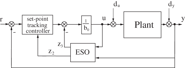
Figure 8: Block diagram of the simulation scheme

5.1 Disturbance Rejection and Set-Point Tracking Performance Analysis

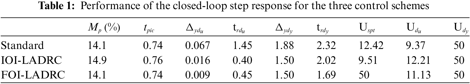
Figs. 9 and 10 show simulation results obtained using the three control schemes and Tab. 1 summarize the main characteristics of the obtained results. Where Mp(%) is the overshoot. tpic is the time corresponding of the first peak (it measures the controller stability to react to changes in the set-point). Δydu is the deviation of the output due to the disturbance on the input. ttdu is the corresponding disturbance rejection time. Δydy is the deviation of the output due to the disturbance on the output. trdy its corresponding disturbance rejection time. Uspt is the maximum value of the control signal required to the set-point tracking. Udu and Udy are the maximum value of the control signal necessary to reject the disturbance on the input and the disturbance on the output, respectively. We notice that:

•   About the set-point tracking, the results obtained using the three control schemes are similar since they all make it possible to achieve the control objectives, namely an overshoot of approximately 14% and the same peak time, and therefore the same settling time.

•   Concerning the external disturbance du(t), however, these results show that the IOI-LADRC and FOI-LADRC are almost the same, but they are both better than the standard order. Indeed, the deviation on the output is only 0.9% and 1.6% for the IOI-LADRC and FOI-LADRC schemes and the time needed to reject this disturbance is of the order of 0.4, while, the deviation on the output is within the range of 6.7 with a disturbance rejection time of about 1.45 for the standard LADRC.

•   Concerning the disturbance on the output, the difference is even more obvious since for the IOI-LADRC and FOI-LADRC, the deviation is only 50% and the output returns to its value after 0.3 whereas with the standard LADRC, the deviation is also 50%, but the time needed to return the output to its initial value is much greater for the standard LADRC since it is 2.32, only 2.01 and 1.69 of the IOI-LADRC and FOI-LADRC respectively.

•   For the control signal, these results show that the FOI-LADRC is the least efficient because it consumes the most energy since the maximum value of the control signal is always the highest. This result was expected because fractional-order controllers are known to be more nervous than integer-order controllers.

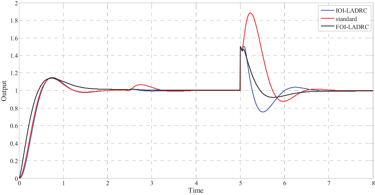
Figure 9: Closed-loop step response with external disturbance on the input at t=2.5 and on the output at t=5

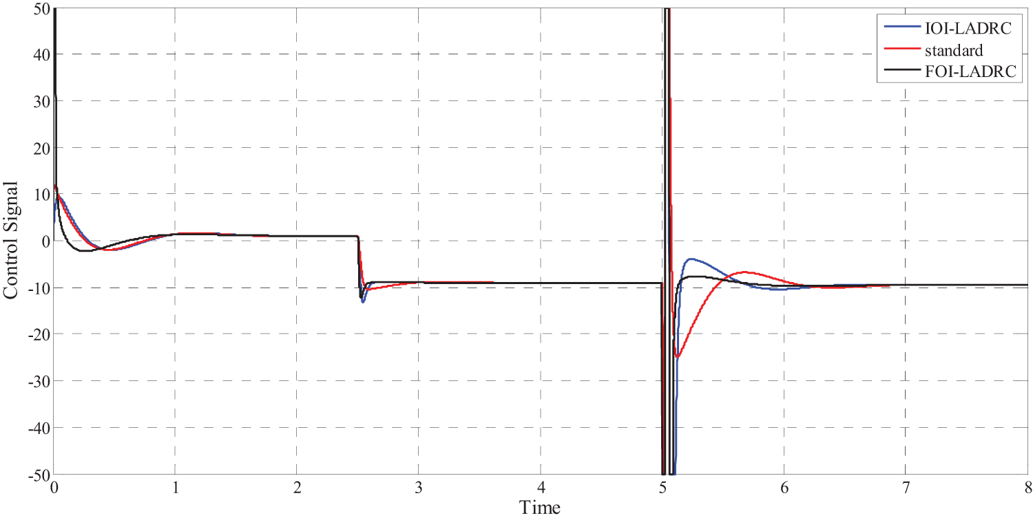
Figure 10: Control signal for the three control schemes

5.2 Influence of b on the Control System Performance

To show the robustness of the three control schemes relative to the gain b, its value is changed to show its effect on the set-point tracking as well as on the rejection of external disturbances du(t) and dy(t). The values of b for which the system becomes unstable are also required. Fig. 11 shows the results obtained with the standard LADRC, Fig. 12 shows those obtained with the IOI-LADRC and Fig. 13 shows those obtained with the FOI-LADRC for b=0.1,0.5,1,2,3. Fig. 13 also shows zooms on the closed-loop step response and the evolution of the output according to the two disturbances.

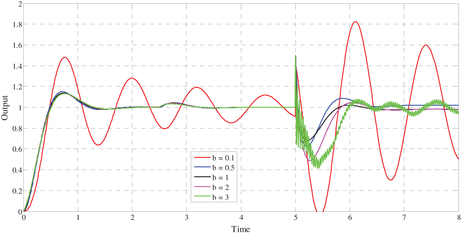
Figure 11: Influence of the variation of b on the performance of the standard LADRC

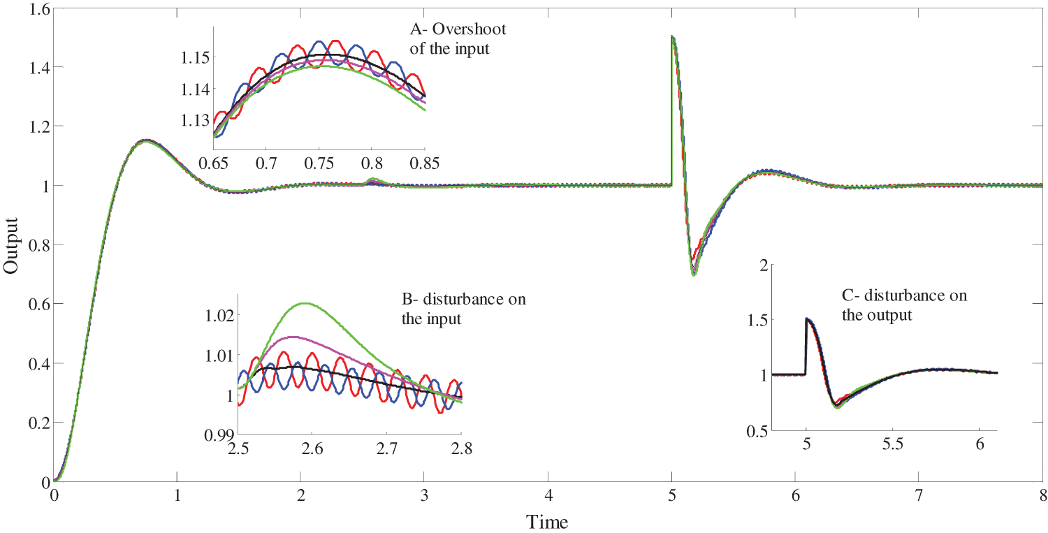
Figure 12: Influence of the variation of b on the performance of the IOI-LADRC

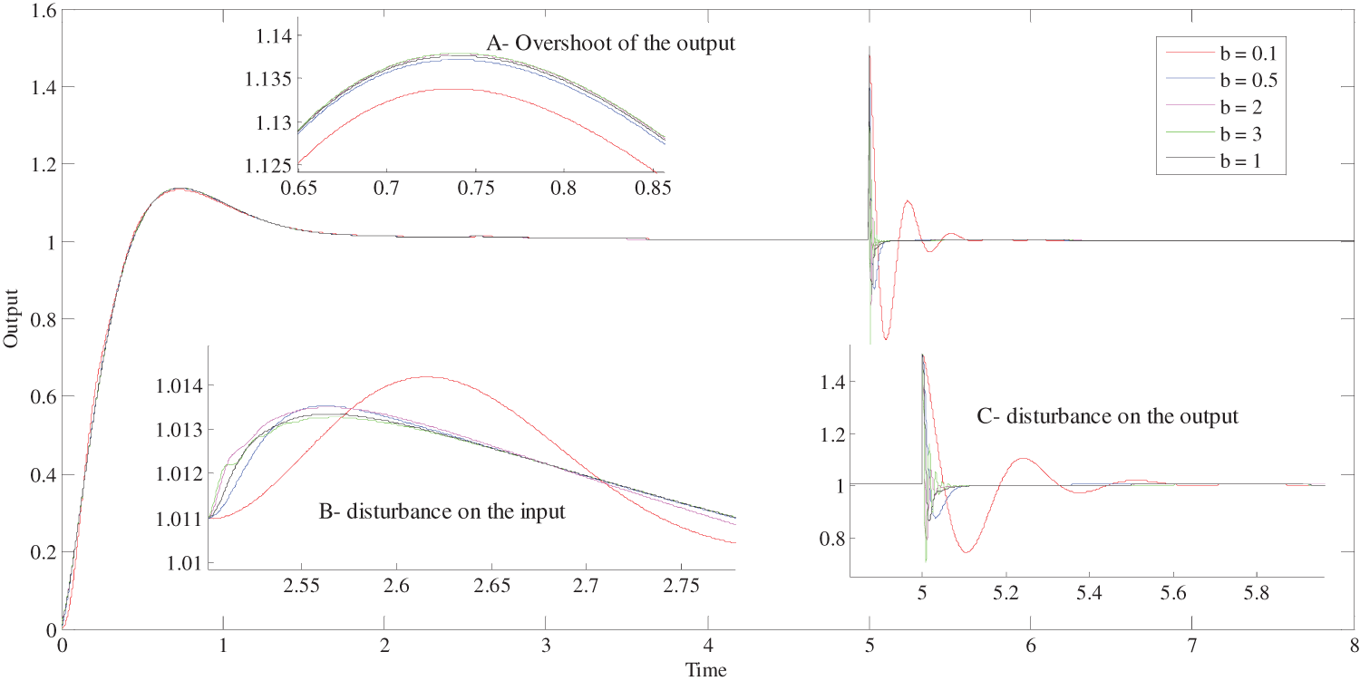
Figure 13: Influence of the variation of b on the performance of the FOI-LADRC

First, for the variation limits of b for which the closed-loop remains stable, we found that the standard LADRC maintains the stability of the closed-loop for 0.07<b<4.15, the range of variation of b is 0.04<b<8.43 for the IOI-LADRC; whereas for theFOI-LADRC, this range of variation is 0.02<b<0.1. Regarding the influence of b on the closed-loop performance, the results shown in Figs. 11–13 clearly illustrate the superiority of the FOI-LADRC compared to the two other LADRC based schemes.

5.3 Closed-Loop Robustness Relative to the Set-Point Tracking Controller Gain Variation

To show the superiority of the FOI-LADRC structure, and the iso-damping property that it is able to obtain, Fig. 14 illustrates the closed-loop step response when the gain kr of the set-point tracking controller changes (Three values of kr are considered: the nominal value, 1.5 and 0.5 times this value) (the standard LADRC is in red color, the IOI-LADRC is in blue color and FOI-LADRC is in black color). Fig. 14 shows that the overshoot of the closed-loop step response changes for the standard LADRC and the IOI-LADRC structures (the overshoot is same for the two control schemes). However, it is insensitive to the variations of kr when the FOI-LADRC structure is used.

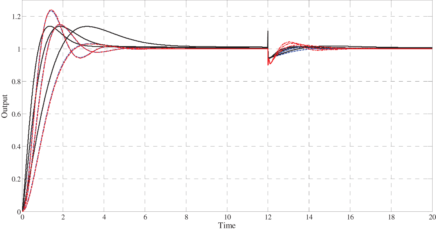
Figure 14: Robustness of the Standard LADRC, the IOI-LADRC and the FOI-LADRC relative to kr

6  Implementation on a Cart-Pendulum System

To illustrate the LADRC control schemes and verify the performance of the proposed FOI-LADRC, compared to the standard LADRC and the IOI-LADRC structures, the cart-pendulum system is a very interesting example because it involves the movement of two interacting systems and its modeling is relatively complex. Indeed, the cart’s motion affects the pendulum and vice-versa. As the goal is to control the position of the cart, the movement of the pendulum is considered to be an internal and a permanent disturbance. The experimental testbed is shown in Fig. 15 [12,28]. Two pendulums are attached to the cart and are able to rotate freely. The movement of the cart causes oscillations of the pendulums. Inversely, the swing of the pendulums disrupts the movement of the cart in a sinusoidal way. The force that allows the cart to move is obtained using a DC motor. The voltage applied to the motor is the control signal and the cart position on the rail is the controlled variable. An advantech PCI1711 card interfaces the experimental hardware with a PC and the control law is implemented in a Matlab/Simulink environment. The sampling time is 0.001 s.

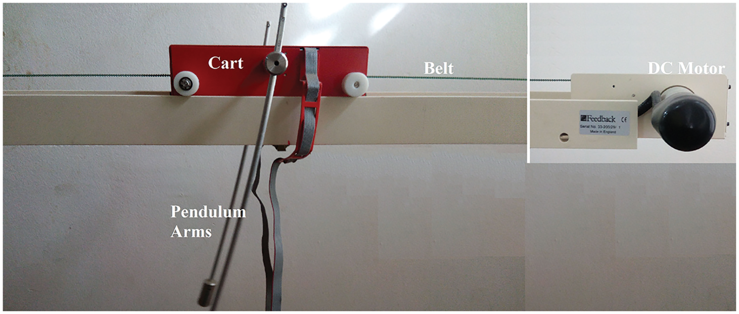
Figure 15: Experimental testbed of the cart-pendulum system

To evaluate and compare the performance of the two LADRC structures, design parameters of the observer are: ω0=100 rad/s and b0=10. For the standard LADRC and the IOI-LADRC, the set-point tracking controller is designed based on the reference model (48) with ωn=3 rad/s and z=0.9 (a third pole pr=50 is added to design the set-point tracking controller of the IOI-LADRC structure). To get similar transient performance, the FOI-LADRC is designed based on the model (50) where τc=0.5 s and λ=0.05. But, because the sampling time is 0.001 s, the time constant of (50) is T=τc/20=0.025 s. CRONE approximation method is used to implement the fractional-order integral action in the frequency range [10−450] with 10 cells.

The reference positions are:+0.2 m at t=0 s, −0.2 m at t=5 s, and 0 at t=10 s. In addition, an external disturbance is applied around t=15 s by tapping the cart manually. Fig. 16 illustrates the experimental results obtained (the standard LADRC is in red color, the IOI-LADRC is in blue color and FOI-LADRC is in black color). This figure shows the cart position, the evolution of the control signal as well as the estimation of the generalized disturbance. A zoom of the disturbance rejection is also highlighted. Tab. 2 summarizes the performances of the three control schemes for the three steps of the reference signal. Mp(%) is the overshoot, Um(V) is the maximum value of the control signal and fm is the maximum variation of the estimated generalized disturbance.

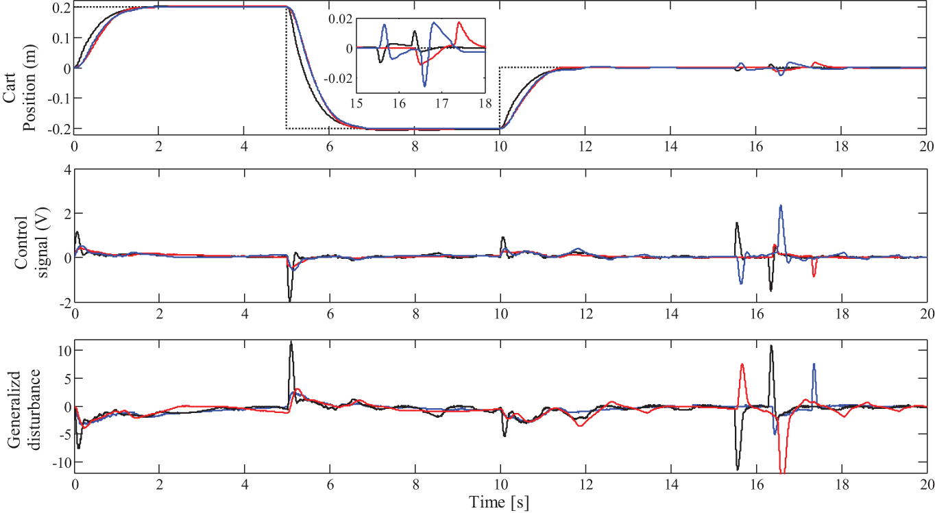
Figure 16: Closed-loop behavior of the Standard LADRC, IOI-LADRC and the FOI-LADRC

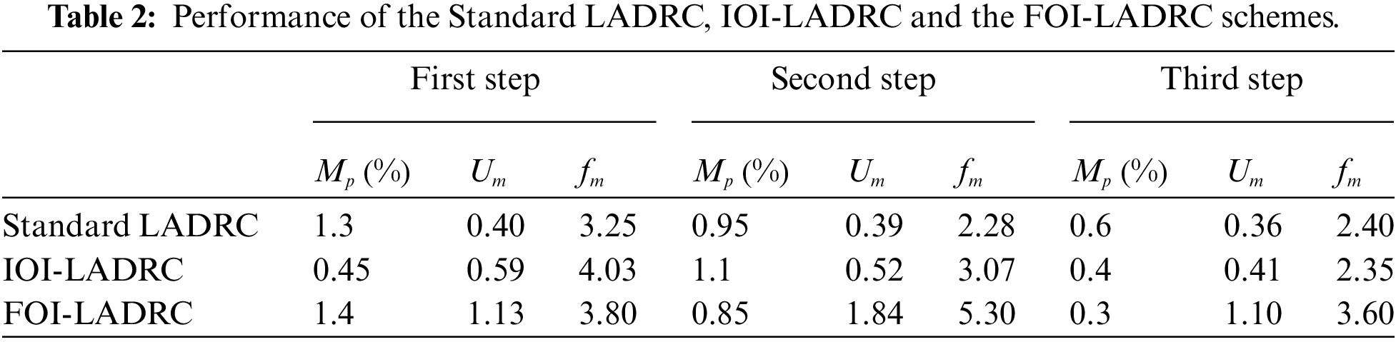
Fig. 16 and Tab. 2 show that the cart tracks the desired position with a small overshoot for all control schemes. The generalized disturbance, the internal as well as the external disturbances have been well estimated and compensated by the three LADRC structures. Note that, when there is a change in the output, (whether due to the set-point or the external disturbance), the generalized disturbance changes accordingly. This means that the observer estimates these changes well. The variation in the generalized disturbance and the fact that there is no change in the set-point or external disturbance, as will be mentioned later, are due to the oscillations of the pendulum, which are considered as internal disturbances. Note also that the control signal is more important for the FOI-LADRC structure. This is explained by the fact that the transient response obtained by theFOI-LADRC is slightly faster. This result are expected because fractional-order systems are known for their nervousness at startup and their slow steady state performance.

A comparison of the three LADRC structures is also made by studying their robustness against the variations of the set-point controller parameter and the variations of a parameter of the cart-pendulum system. On the one hand, to show the robustness of the LADRC schemes against the set-point controller parameter variations, three values of the parameter kr are considered: the tuned value and the value obtained by multiplying this tuned value by 0.5 and by 1.5. On the other hand, to show the robustness of the studied LADRC schemes against the parameters of the controlled system, the three LADRC structures are evaluated for two values of the cart weight: the normal value 2.3 kg and the value modified by adding on the cart an additional metal mass weighing 0.72 kg.

The obtained results are illustrated in Figs. 17, 18 and Tab. 3 for the standard LADRC scheme, in Figs. 19, 20 and Tab. 4 for the IOI-LADRC scheme and Figs. 21, 22 and Tab. 5 for the FOI-LADRC scheme.

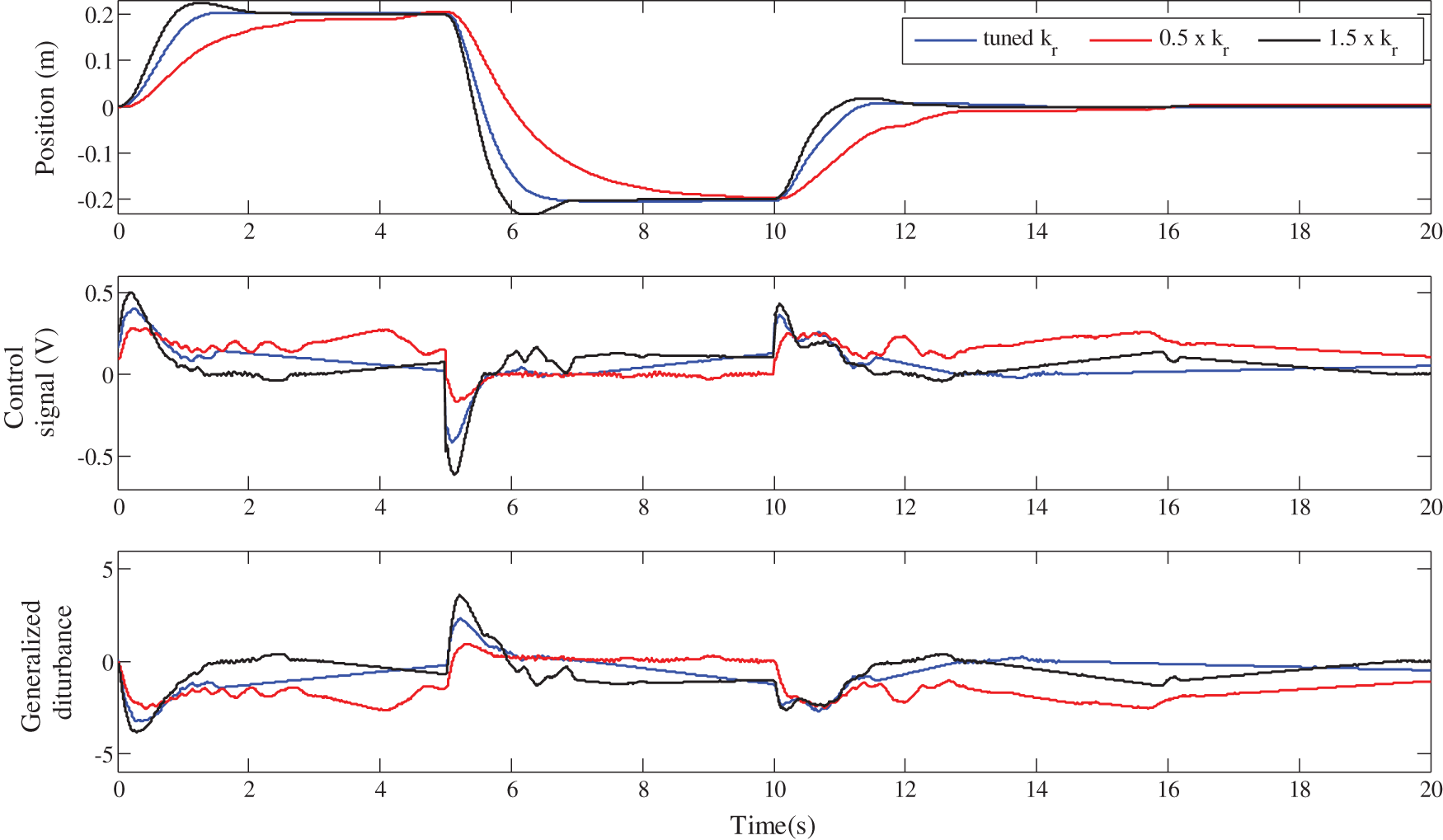
Figure 17: Robustness of the standard LADRC against the gain kr

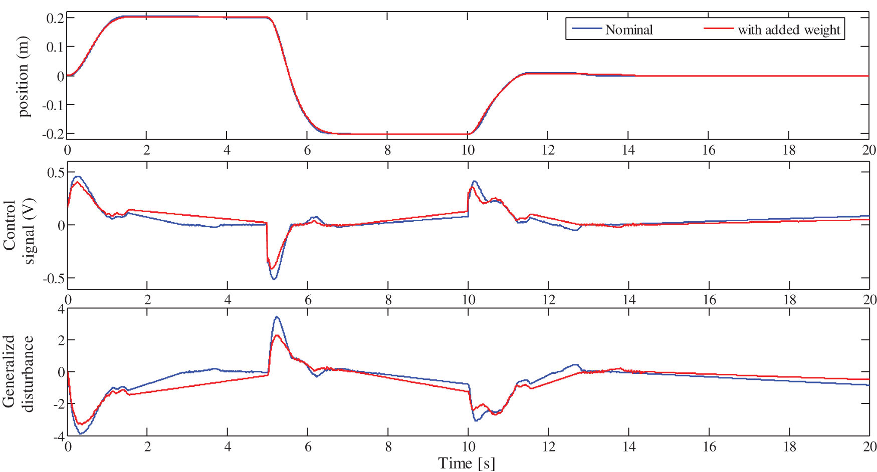
Figure 18: Robustness of the standard LADRC against the cart weight variation

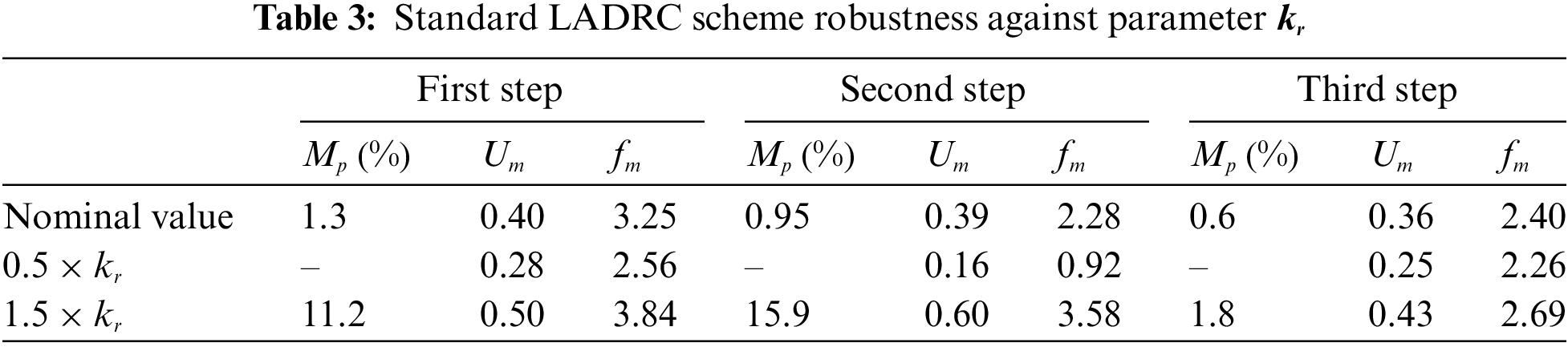
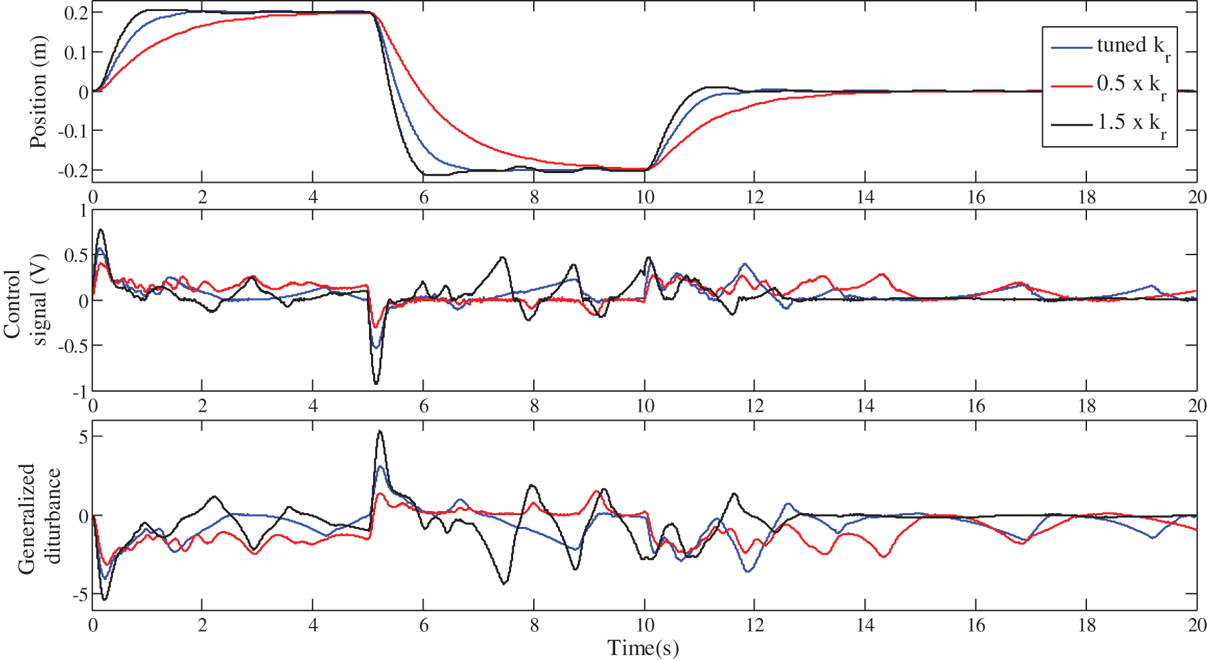
Figure 19: Robustness of the IOI-LADRC against the gain kr

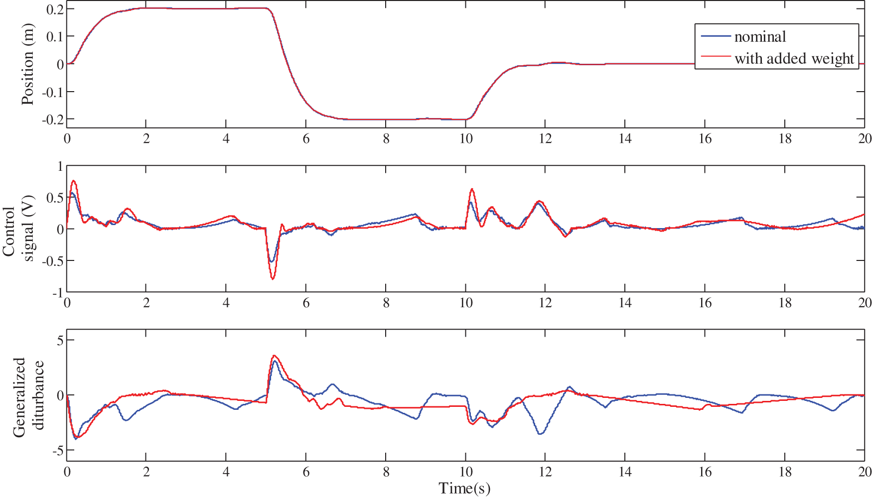
Figure 20: Robustness of the IOI-LADRC against the cart weight variation

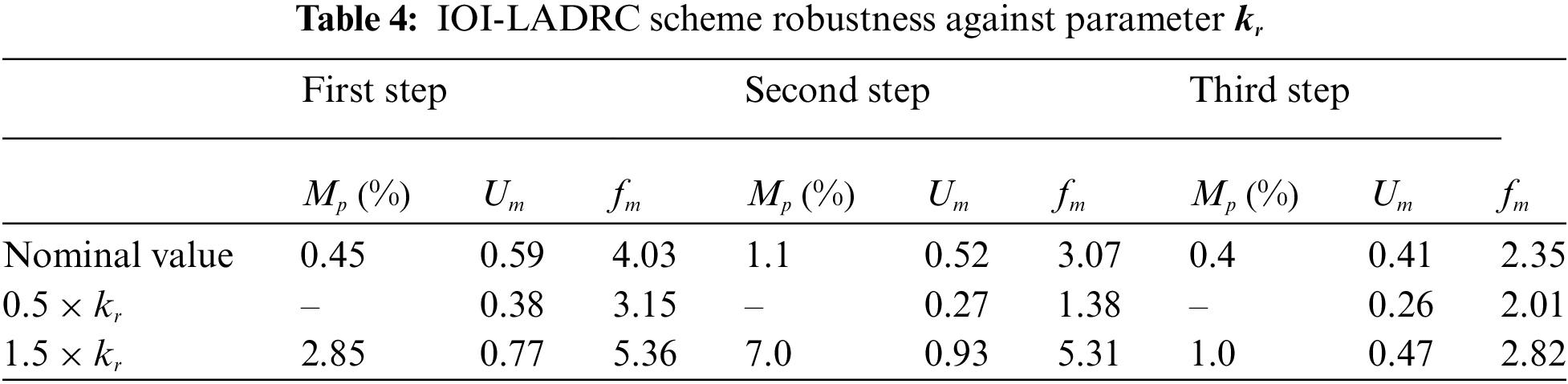
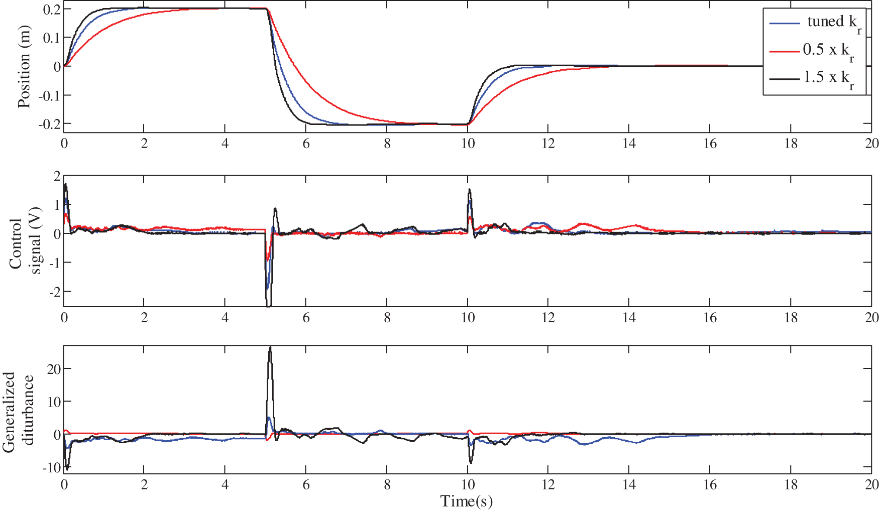
Figure 21: Robustness of the FOI-LADRC against the gain kr

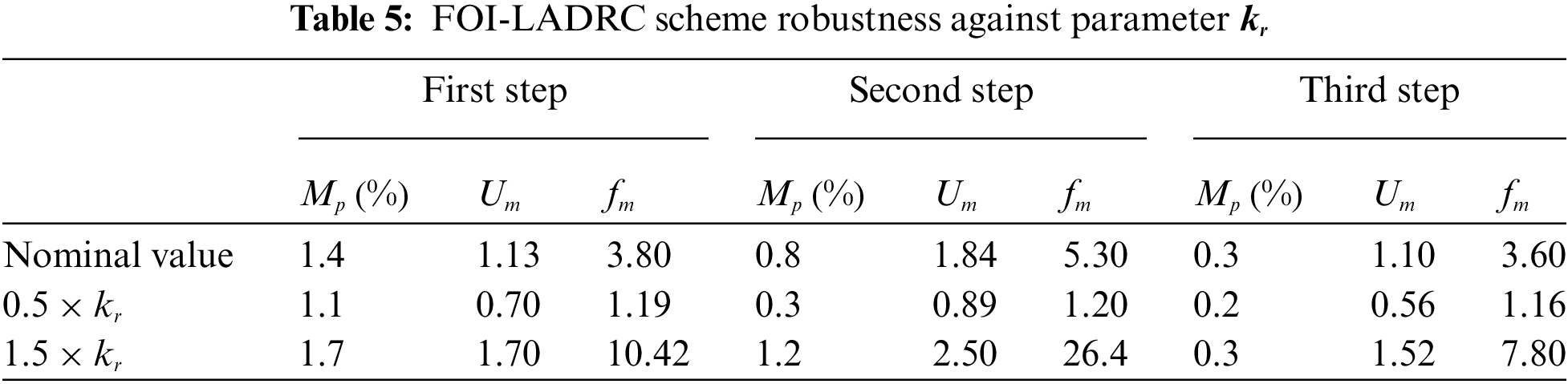
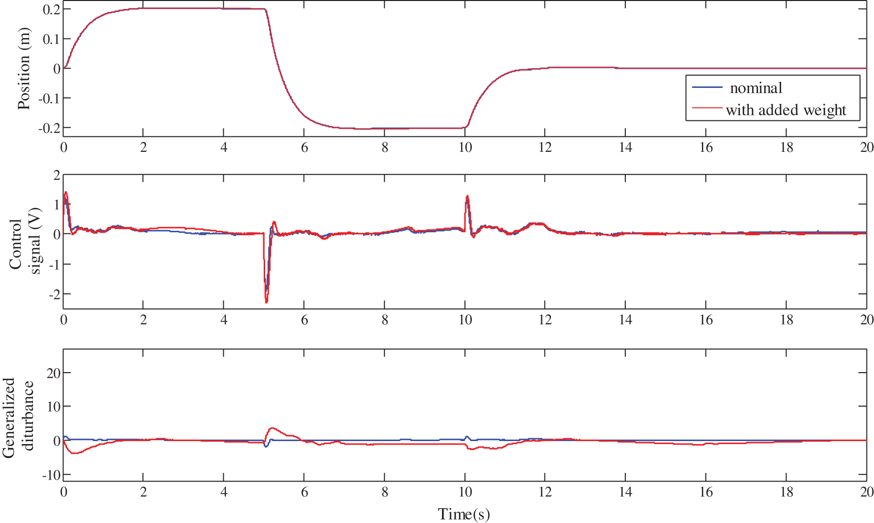
Figure 22: Robustness of the FOI-LADRC against the cart weight variation

Firstly, it should be noted from Figs. 18, 20 and 22, that for the three control schemes, the change on the cart weight has no effect on the evolution of the cart position. This was expected, since the LADRC scheme is a model-free control, which is not based on the controlled system parameters. The evolution of the generalized disturbance illustrates this fact well. Indeed, its evolution is different when the weight of the cart is normal and when it is modified. This difference is due to the influence of the cart weight on the evolution of its position. This is estimated by the observer and then canceled by the control law, which evolves accordingly as shown in these same figures.

Figs. 17, 19, 21 and the performance of the three LADRC schemes summarized in Tabs. 3–5 show that the closed-loop step response with the FOI-LADRC is almost insensitiveto the variations of gain kr, which is not the case with the standard LADRC and the IOI-LADRC. This demonstrates that the use of the fractional-order integral action improves the robustness of the LADRC structure. Nevertheless, this superiority is paid by higher values of the control signal, which is expected.

7  Conclusion

In this paper, the LADRC structure with a fractional-order integral action (FOI-LADRC) is proposed to control a minimum phase stable system. Two main contributions are achieved. From the theoretical point of view, based on the Bode’s ideal transfer function, a novel design method of the set-point tracking controller is proposed for the FOI-LADRC scheme. From a practical point of view, the use of LADRC control scheme is an important contribution since no modeling of the system is needed and all the parameters of the system are not accessible. Nevertheless, a minimal knowledge of the system is necessary. We know for example, that the relative degree of the model of the DC motor position is equal to 2. That is why a third order ESO is used to estimate the generalized disturbance. It is shown by numerical simulation and experiment that the robustness of the FOI-LADRC scheme is superior.

Funding Statement: This project was supported by the Deanship of Scientific Research (DSR), King Abdulaziz University, Jeddah, under grant No. (DF-474-135-1441). The authors, therefore, gratefully acknowledge DSR technical and financial support.

Conflicts of Interest: The authors declare that they have no conflicts of interest to report regarding the present study.

This work is licensed under a Creative Commons Attribution 4.0 International License, which permits unrestricted use, distribution, and reproduction in any medium, provided the original work is properly cited.