DOI:10.32604/cmc.2022.026259
| Computers, Materials & Continua DOI:10.32604/cmc.2022.026259 | |
| Article |
TP-MobNet: A Two-pass Mobile Network for Low-complexity Classification of Acoustic Scene
1NAVER Corporation, Seongnam, 13561, Korea
2Department of Computer Science and Engineering, Sogang University, Seoul, 04107, Korea
*Corresponding Author: Ji-Hwan Kim. Email: kimjihwan@sogang.ac.kr
Received: 20 December 2021; Accepted: 22 February 2022
Abstract: Acoustic scene classification (ASC) is a method of recognizing and classifying environments that employ acoustic signals. Various ASC approaches based on deep learning have been developed, with convolutional neural networks (CNNs) proving to be the most reliable and commonly utilized in ASC systems due to their suitability for constructing lightweight models. When using ASC systems in the real world, model complexity and device robustness are essential considerations. In this paper, we propose a two-pass mobile network for low-complexity classification of the acoustic scene, named TP-MobNet. With inverse residuals and linear bottlenecks, TP-MobNet is based on MobileNetV2, and following mobile blocks, coordinate attention and two-pass fusion approaches are utilized. The log-range dependencies and precise position information in feature maps can be trained via coordinate attention. By capturing more diverse feature resolutions at the network's end sides, two-pass fusions can also train generalization. Also, the model size is reduced by applying weight quantization to the trained model. By adding weight quantization to the trained model, the model size is also lowered. The TAU Urban Acoustic Scenes 2020 Mobile development set was used for all of the experiments. It has been confirmed that the proposed model, with a model size of 219.6 kB, achieves an accuracy of 73.94%.
Keywords: Acoustic scene classification; low-complexity; device robustness; two-pass mobile network; coordinate attention; weight quantization
The goal of acoustic scene classification (ASC) is recognition and classification using audio signals to identify an environment [1], thereby enabling a wide range of applications including surveillance [2], intelligent wearable devices, and robot sensing services. As in other fields, ASC problems have been approached using deep learning, including deep neural networks [3,4], convolutional neural networks (CNN) [5], recurrent neural networks [6], and convolutional recurrent neural networks [7]. Of these, CNNs are used widely for ASC problems because they perform reliably when using spectrogram images of audio data for training [8]. There have been various ASC studies using CNNs. Piczak et al. [5] introduced CNNs into ASC and environmental sound classification and evaluated their potential, and since then various CNN models have been proposed for ASC [9,10] and there have been several studies of low-complexity CNN models [11–13].
Additionally, model complexity and device robustness are important issues when applying ASC systems in the real world, and ASC systems are also used in low-performance devices such as mobile devices. In this paper, we propose a two-pass mobile network for low-complexity classification of the acoustic scene, named TP-MobNet. MobileNetV2 [12] and MobNet [14] are the foundations for TP-MobNet. Inverse residuals and linear bottlenecks are used, just as they were in the two preceding models. In addition, the proposed two-pass approaches and coordinated attention are used. The proposed two-pass technique has an impact on feature resolution training. Also, weight quantization is used to reduce model size. The TAU Urban Acoustic Scenes 2020 Mobile development set [15] was used for all of the experiments. The proposed TP-MobNet in the single model and ensemble model showed 72.59% and 73.94% accuracy, respectively, with model sizes of 126.5 and 219.6 kB.
This paper is organized as follows. Section 2 presents related work involving various ASC methods. Section 3 analyzes in detail the proposed method of TP-MobNet using coordinate attention. Finally, Sections 4 and 5 present the experimental results and conclusions, respectively.
The use of CNN has been widely explored over the years in the task of ASC. In this section, we describe various modifications in CNN or additional that have been proposed to improve the performance of ASC. Starting with the CNN-based ASC model in Sections 2.1, 2.2 describes the mobile-network-based ASC model. It then proceeds to explore previous studies involving the combination of attention and two-pass methods with CNN and mobile-network models.
As part of the detection and classification of acoustic scenes and events (DCASE) series, ASC appears in every edition of task [16]. The baseline system for DCASE 2021 Task 1a task implementation uses a deep CNN, which was proposed by Valenti et al. [17] as a training strategy that takes full use of the limited datasets available. Batch normalization and adjustments to layer widths were applied to the original system. There have been several entries based on adaptations of the CNN-based network since Valenti et al. [17] recommended employing a CNN to identify short sequences of audio data in the DCASE challenge.
Dorfer et al. [18] proposed a system based on a CNN trained on spectrograms, which consisted of two convolutions and one fully connected layer, the entire input segment. Additionally, they also optimized their models using hyperparameter tuning.
2.2 ASC Models Based on Mobile Networks
MobNet was proposed by Hu et al. [14], coupled with a set of CNN-based models and a mix of data augmentation strategies. Time and frequency operations and analysis were specialized by CNN-based systems. MobNet is a mobile network that is heavily based on MobileNetV2. The MobileNetV2 is built on an inverted residual, with bottleneck layers that are typical residual models in reverse order as input and output of the residual block [12]. The inverted residual block expands the input dimensions rather than lowering them, preserving information that might otherwise be lost in a typical residual model. To filter features in the intermediate expansion layer and reduce the model's complexity, MobileNetV2 employs lightweight depth-wise convolutions [12]. To retain representational power, it then reduces nonlinearities in the narrow layers. As a result, MobileNetV2 keeps its great accuracy while lowering its complexity.
2.3 ASC Models Based on Attention and Two-pass Method
Cao et al. [19] proposed using attention to maintain details from the feature map. ResNet with an inverted residual block was the basis for their proposed model. They included spatial attention and channel attention module to the model to compensate for aspects such as crucial features that could be lost in the model. In the feature map, the channel attention performs global average and max pooling, then feeds the features into a two-layer neural network. Following the activation functions, a weight coefficient is generated to multiply with the feature map. The spatial attention, on the other hand, executes maximum and average pooling on a single channel dimension. This is applied to each channel separately before being concatenated. The concatenation results are then sent into a convolution with a sigmoid activation function to produce a weight coefficient, which is subsequently multiplied by the feature map.
McDonnell et al. [20] proposed late fusion, which involves combining two CNN paths before the network output. The input spectrogram is split into two parts: high frequencies and low frequencies, which are then averaged over overlapping views rather than global views, and the two paths are then merged in the final layer.
3 Two-pass Mobile Networks Using Coordinate Attention
We designed TP-MobNet based on MobNet and MobileNetV2, as described in Sections 3.1 and 3.2. In addition, coordinate attention is added, and the detailed mechanism is described in Section 3.3. Also, Section 3.4 describes the weight quantization.
The proposed baseline model, as shown in Tab. 1, is mostly made up of mobile blocks. To input features, the first two-dimensional convolution and three mobile blocks are employed. The mobile blocks are built for channel dimensions, and each has 32, 48, or 64 channels. The features are then activated using the batch normalization and ReLU activation functions. The features are then given coordinate attention after one convolution and dropout. Finally, the coordinate attention features are supplied into the final convolution, where pooling and softmax functions are applied.
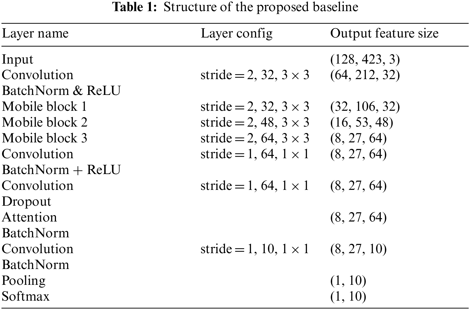
Based on MobileNetV2, the mobile blocks are subjected to linear bottlenecks and inverted residuals. As shown in Tab. 2, a mobile block consists of three bottlenecks: three bottleneck layers: one bottleneck, and two residual bottlenecks. The preceding bottleneck's output features are linearly transmitted to the next bottleneck without being activated.
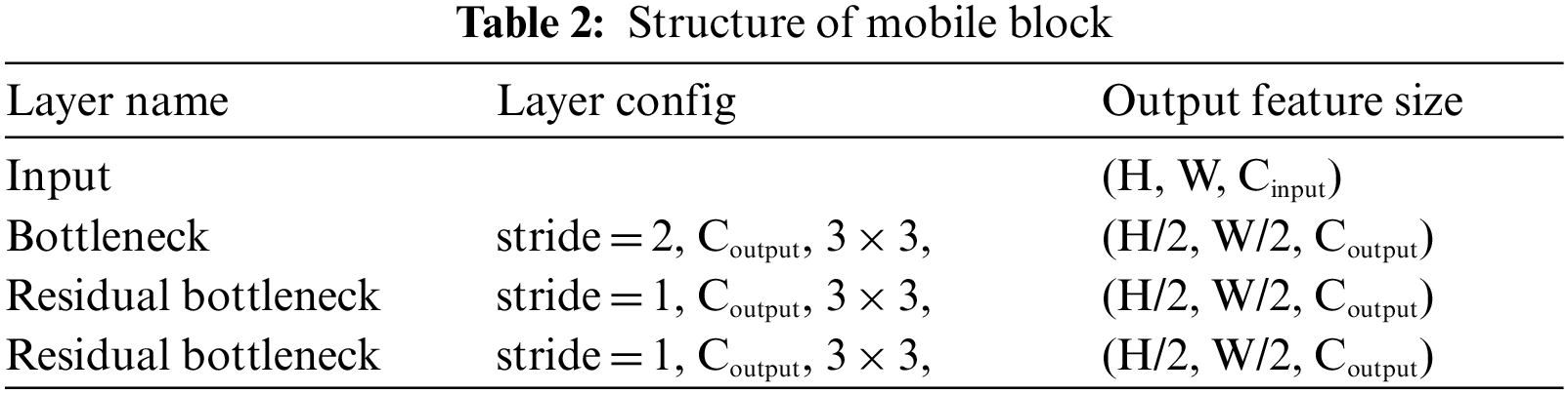
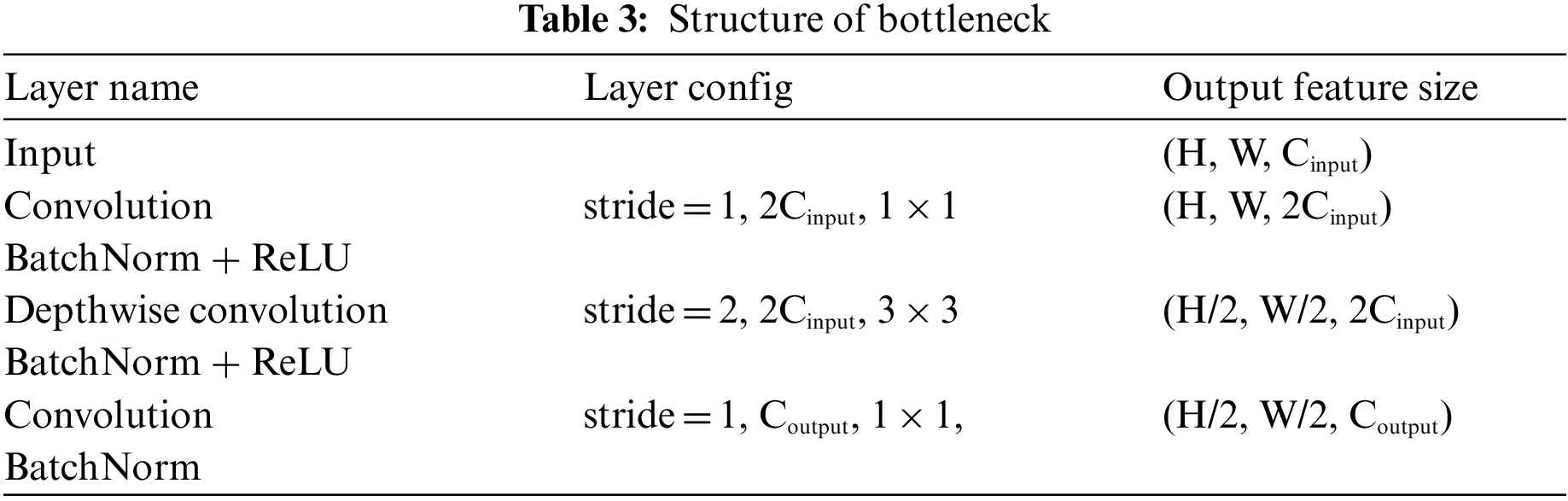
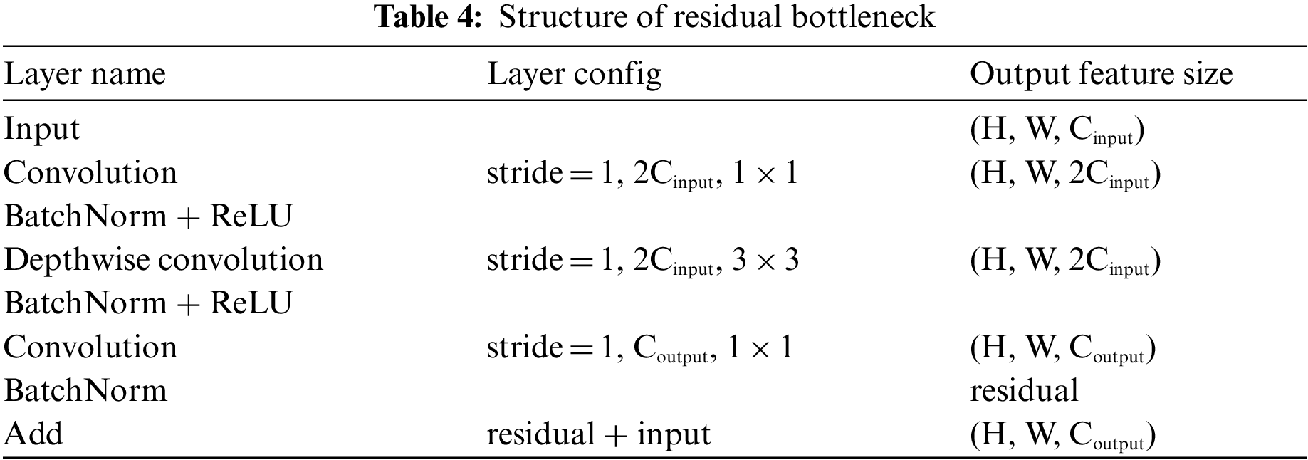
The feature dimension is lowered by half in the bottleneck with stride 2 through the depth-wise convolution, as shown in Tabs. 3 and 4. Alternatively, in the residual bottleneck, which uses skip connections, the feature dimension is retained. In addition, all bottlenecks are also applied to channel expansion at the first convolution, and they are recovered at the last convolution.
For the proposed TP-MobNet, fusion approaches are used. Two convolution output features are fused in the first convolution (early fusion), and the output features of the last convolution are divided in half, as shown in Tab. 5 and Fig. 1. Coordinate attention is given to one side of the divided features but not the other. After applying pooling and softmax to both output features, the interpolation is processed (late fusion).
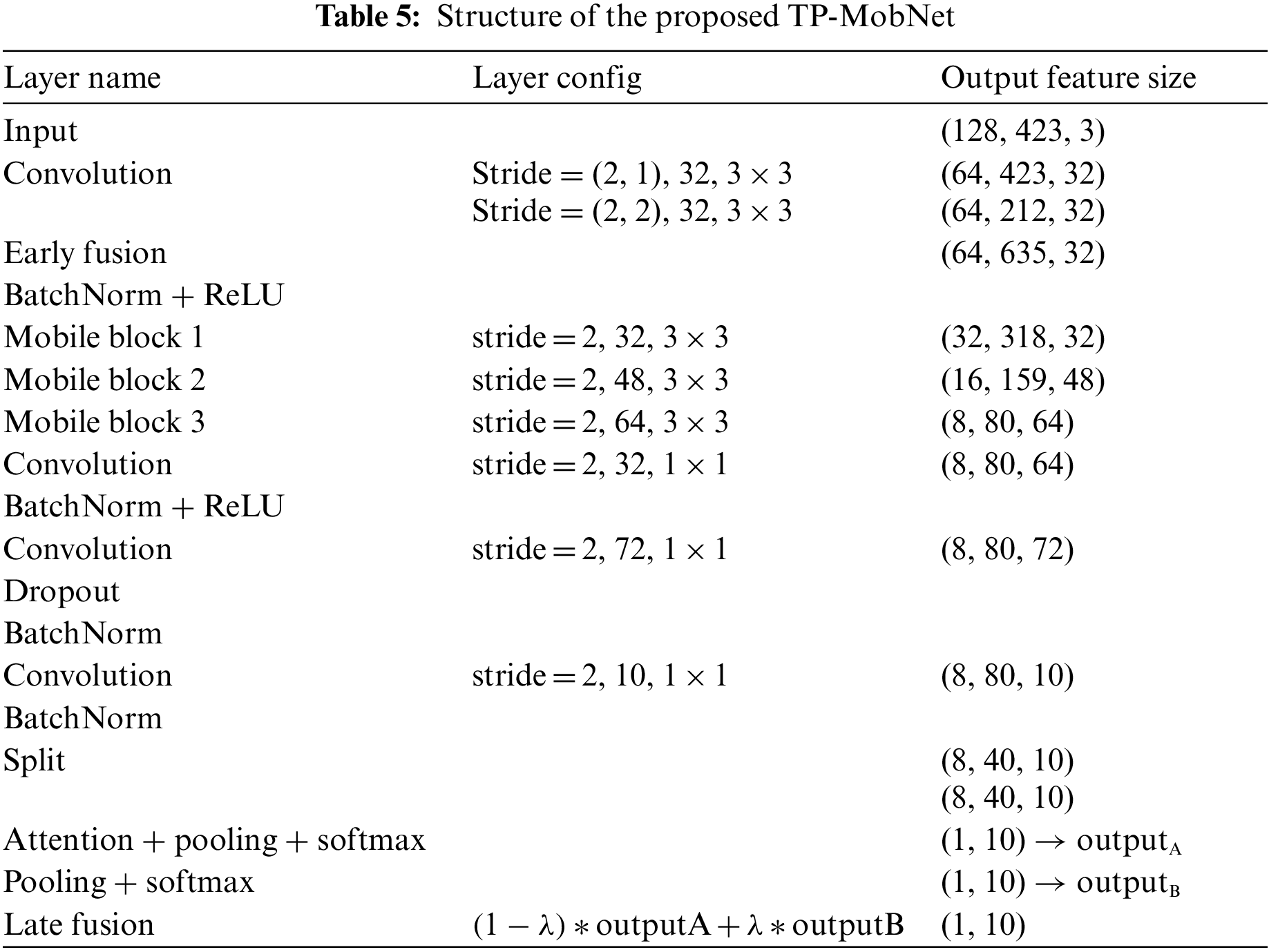
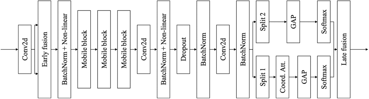
Figure 1: Structure of the proposed TP-MobNet
The reason why two fusions are applied is as follows. The output of the convolution is computed only by a small window. Depending on the value of the small window, overfitting may occur. Therefore, early fusion is applied to reduce overfitting caused by windows. And coordinate attention has a low capability for channel relationships. Late fusion is applied to capture the channel relationship in the final output.
The experiment demonstrated that when early fusion and late fusion were combined, they had similar effects on the ensemble. For the first convolution, we used several strides. In contrast to stride (2, 1) which can only be fused along the time axis, stride (2, 2) can be fused in both directions. It was confirmed that proper performance could only be achieved when the axis of early fusion was the same in split operations.
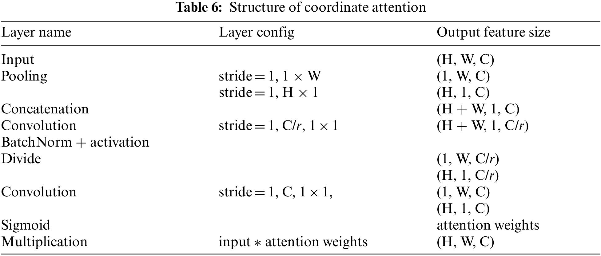
We utilize coordinate attention [21], a new method of integrating positioning information into channel attention for mobile networks. In contrast to squeeze-and-excitation channel attention [22], coordinate attention is decomposed into two feature encodings by bi-directional average pooling. It can be used to train long-range relationships as well as precise position information in feature maps.
As shown in Tab. 6, two two-dimensional average poolings are used for the X and Y axes. Thereafter, after the output features have been concatenated, the number of channels is adjusted based on the reduction ratio r. Following BN, a swish activation and ReLU6 function are used as activation. For each attention weight, the data is divided into X and Y axes. The attention weights are applied to the input features by multiplying them.
Our trained model is quantized for efficient integer-arithmetic-only inference [23]. Converting a 32-bit fixed-point operation to a low-precision 8-bit operation can boost the speed of the CNN model while reducing its weight [3]. The TensorFlow Lite converter in TensorFlow Lite [24] supports an 8-bit quantization technique.
We evaluated the proposed TP-MobNet using the TAU Urban Acoustic Scenes 2020 Mobile dataset. Sections 4.1 and 4.2 describe the specifications and processing of this dataset, Section 4.3 describes the training in detail, and Section 4.4 presents the experimental results.
A development dataset and an evaluation dataset make up the TAU Urban Acoustic Scenes 2020 Mobile dataset (the evaluation dataset is not published). Airport, retail mall, metro station, street pedestrian, public plaza, street traffic, tram, bus, metro, and park are the acoustic scene classifications in the dataset. The development dataset comprises 10-s segments recorded with three genuine devices (A–C) and six simulated devices (S1–S6), as shown in Tab. 7. The overall length and number of segments are respectively 64 h and 23,040.
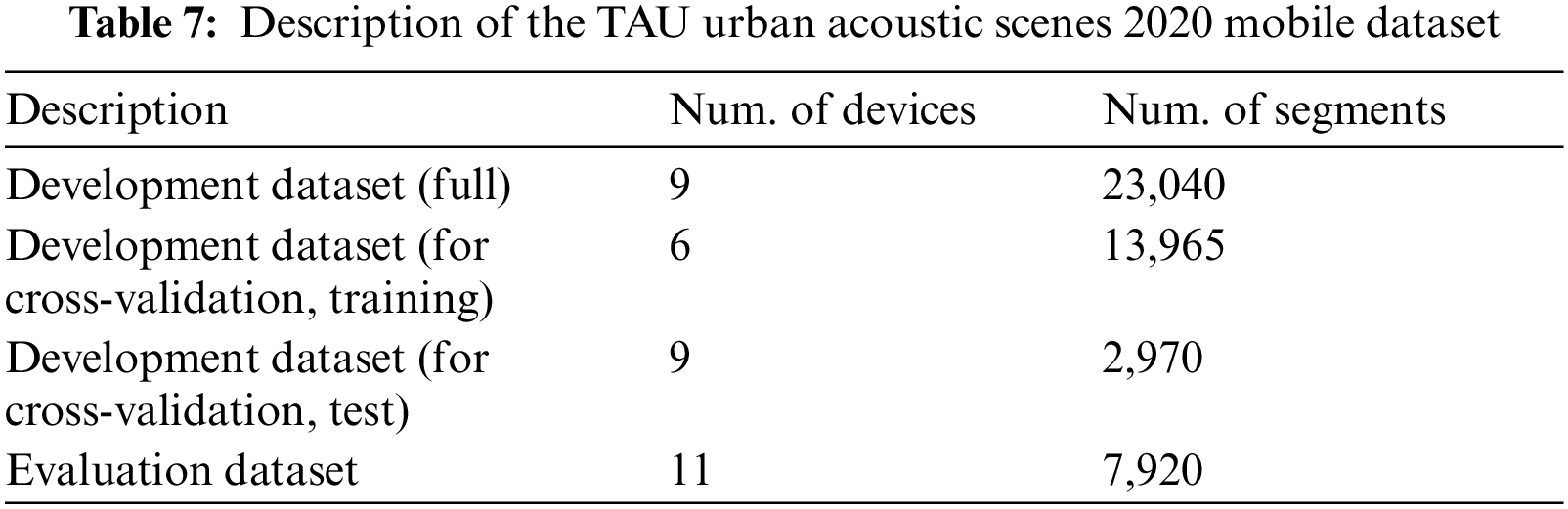
The development dataset is separated into 70 percent training and 30 percent test for the cross-validation setup. Several segments aren't used for the balanced test dataset in this situation. In addition, the test dataset contains only three simulated devices (S3–S6). The training and test dataset each of 13 965 and 2970 segments, respectively. The evaluation dataset consists of 10-s segments recorded with 11 devices, one of which is a real device (D) and four of which are simulated (S7–S11). There are 7920 segments in total (the evaluation dataset is not published).
4.2 Data Preprocessing and Augmentations
All of the audio segments were recorded in mono with a sampling rate of 44 kHz and a 24-bit resolution per sample. 2048 FFT points were done for every 1024 samples in each 10-s input segment, and a power spectrum was derived. In that instance, there were 431 bins in one power spectrum. Then, with 128 frequency bins, log-Mel filterbank characteristics were recovered, and mean and variance normalization was done to each frequency bin. The normalized log-Mel filterbank features were also used to produce delta and delta-delta, which were then stacked into the channel axis. As a result, one of the input features was in the shape of 128 × 423 × 3.
Mixup [25], spectrum augmentation [26], spectrum correction [14], pitch shift, speed change, and mix audios were used as data augmentation methods for the features. In the training procedure, mixup and spectrum augmentation were applied. A mixup with an alpha value of 0.4 was applied to each mini-batch of input features, which were randomly masked for time and frequency.
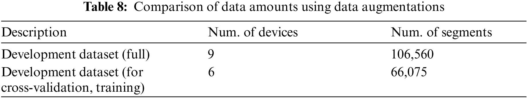
Before training, other augmentation methods like spectrum correction, pitch shift, speed change, and mix audios were used. Averaging the spectra from all training devices except device A was used to generate reference device spectra for spectrum correction. The reference device spectrum was used to adjust the spectra of device A. In addition, the acoustic signals of all training datasets were enhanced by padding and cropping to randomly shift the pitch and change the speed. In addition, acoustic signals from the same classes were mixed at random. As seen in Tab. 8, these data augmentations enhanced the total amount of training data.
TensorFlow 2.0 and Keras were used in all of the experiments presented here. With a 0.9 momentum weight and a 10 − 6e decay, the optimizer employed stochastic gradient descent. Categorical cross-entropy loss was also employed. With a batch size of 32, all of our models were trained for 256 epochs. The learning rate was initially set to 0.1. The learning rate was reset at epochs 3, 7, 15, 31, 127, and 255. We selected the validation point with the highest accuracy as the best model. The late fusion interpolation value was set to 0.5.
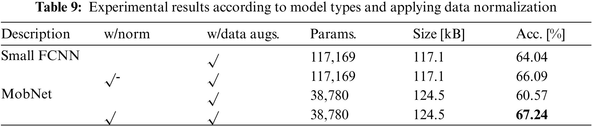
Tabs. 9–14 provide the experimental results and details. Tab. 9 shows the experimental findings broken down by model type and data normalization. As a starting point, we constructed two models. Small FCNN [17] and MobNet [17] are two of them. Small FCNN had an accuracy of 64.04% and 66.09%, depending on whether or not data normalization was used. The accuracy standards for the proposed MobNet, on the other hand, were 60.57% and 67.24%. When both models were normalized, it was confirmed that they performed better.
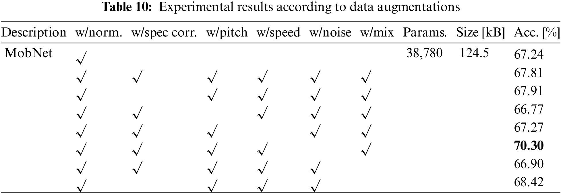
The experimental results are presented in Tab. 10 by the method of data augmentation. Ablation studies were carried out using five distinct augmentation strategies, with data normalization used as a default. As a result of the experiment, the best performance was achieved when simply noise was excepted, with an accuracy of 70.30%.
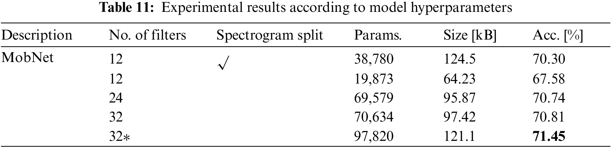
The experimental results are presented in Tab. 11 according to the MobNet hyperparameters. The performance of the mobile block was confirmed in particular based on the difference in the number of initial filters. To begin, the process of separating the spectrogram into two splits and feeding it to the network was eliminated to decrease parameters. The accuracy climbed to 70.81% Tab when the number of filters was raised to 32. It was validated that the accuracy standard with 121.1 KB was increased to 71.45% using the same number of filters (displayed as 32*) as the model proposed in 1.
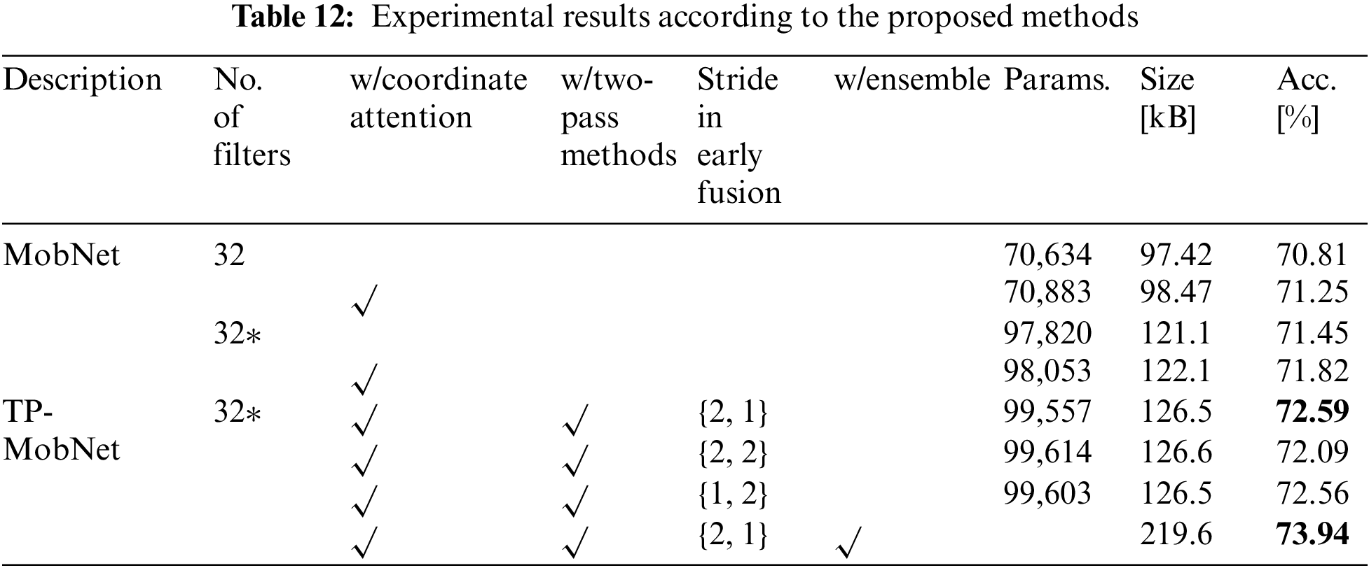
The performance evaluation of several proposed strategies is presented in Tab. 12. The accuracy was 71.82% in the case of the proposed TP-MobNet with two-pass techniques, and 72.59% in the stride 2, 1 combination in the case of the proposed TP-MobNet with two-pass methods. In this example, we confirmed that it had the best performance of the single models proposed, with 99,557 parameters and a size of 126.5. Various strides were used, and two models were combined to corroborate the 73.94% accuracy.
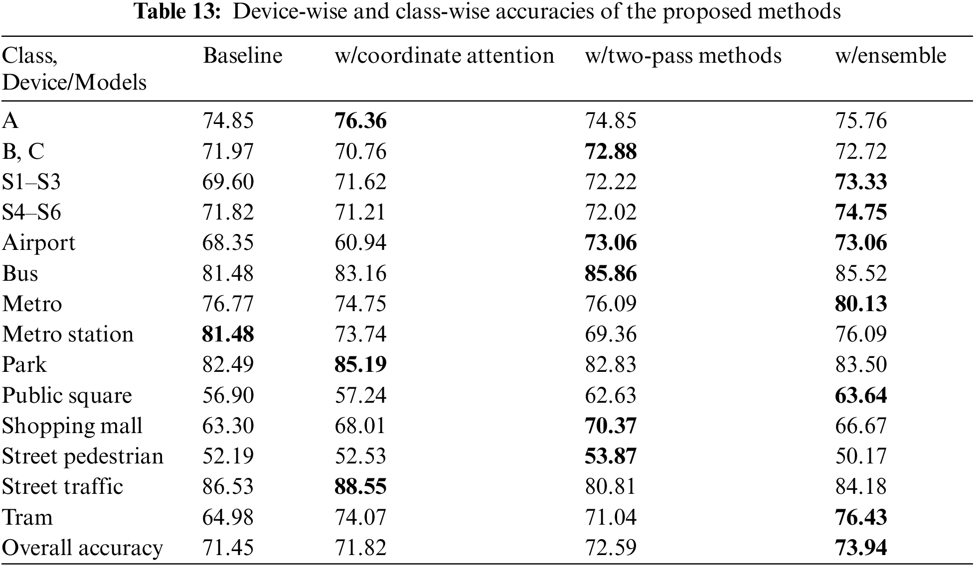
Tab. 13 shows performance device-wise and class-wise. The majority of the proposed approaches’ performances were confirmed to be better than the baseline. It was confirmed that the ensemble model performed better for S4–S6, which is a previously unknown device.
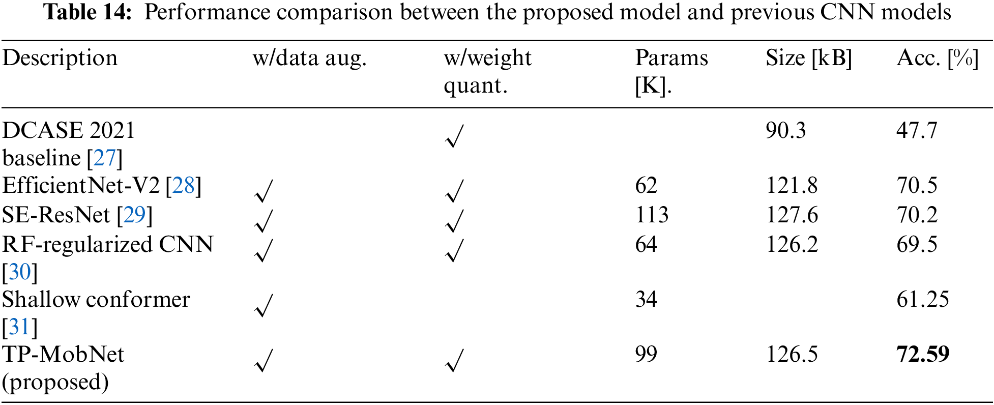
Finally, Tab. 14 compares the performance of previous CNN models and the proposed TP-MobNet. The size of the single model was confirmed to be similar to previous CNN models, but the performance was somewhat enhanced.
In this paper, we propose a two-pass mobile network for low-complexity classification of the acoustic scene, named TP-MobNet. The proposed TP-MobNet includes two-pass fusion techniques in a single model, as well as coordinate attention and weight quantization. Experiments on the TAU Urban Acoustic Scenes 2020 Mobile development set confirmed that our model, with a model size of 219.6 kB, obtained an accuracy of 73.94%.
Funding Statement: This work was supported by Institute of Information & communications Technology Planning & Evaluation (IITP) grant funded by the Korea government (MSIT) [No. 2021-0-0268, Artificial Intelligence Innovation Hub (Artificial Intelligence Institute, Seoul National University)]
Conflicts of Interest: The authors declare that they have no conflicts of interest to report regarding the present study.
1. E. Sophiya and S. Jothilakshmi, “Deep learning based audio scene classification,” in Proc. of Int. Conf. on Computational Intelligence, Cyber Security, and Computational Models (ICC3), Coimbatore, India, pp. 98–109, 2017. [Google Scholar]
2. Y. Petetin, C. Laroche and A. Mayoue, “Deep neural networks for audio scene recognition,” in Proc. of European Signal Processing Conf. (EUSIPCO), Nice, France, pp. 125–129, 2015. [Google Scholar]
3. V. Vanhoucke, A. Senior and M. Z. Mao, “Improving the speed of neural networks on CPUs,” in Proc. of Deep Learning and Unsupervised Feature Learning NIPS Workshop, Granada, Spain, vol. 1, pp. 4, 2011. [Google Scholar]
4. R. Mu and X. Zeng, “A review of deep learning research,” KSII Transactions on Internet and Information Systems, vol. 13, no. 4, pp. 1738–1764, 2019. [Google Scholar]
5. K. J. Piczak, “Environmental sound classification with convolutional neural networks,” in Proc. of 25th Int. Workshop on Machine Learning for Signal Processing (MLSP), Boston, USA, pp. 1–6, 2015. [Google Scholar]
6. S. H. Bae, I. Choi and N. S. Kim, “Acoustic scene classification using parallel combination of LSTM and CNN,” in Proc. of Workshop on Detection and Classification of Acoustic Scenes and Events (DCASE2016), Budapest, Hungary, pp. 11–15, 2016. [Google Scholar]
7. H. Jallet, E. Cakır and T. Virtanen, “Acoustic scene classification using convolutional recurrent neural networks,” Detection and Classification of Acoustic Scenes and Events (DCASE2017), Virtual, 2017. [Google Scholar]
8. M. Lim, D. Lee, H. Park, Y. Kang, J. Oh et al., “Convolutional neural network based audio event classification,” KSII Transactions on Internet and Information Systems, vol. 12, no. 6, pp. 2748–2760, 2018. [Google Scholar]
9. M. Valenti, A. Diment and G. Parascandolo, “DCASE 2016 acoustic scene classification using convolutional neural networks,” in Proc. of Workshop on Detection and Classification of Acoustic Scenes and Events (DCASE2016), Budapest, Hungary, pp. 95–99, 2016. [Google Scholar]
10. Y. Han, J. Park and K. Lee, “Convolutional neural networks with binaural representations and background subtraction for acoustic scene classification,” Detection and Classification of Acoustic Scenes and Events (DCASE2017), Virtual, 2017. [Google Scholar]
11. A. G. Howard, M. Zhu, B. Chen, D. Kalenicheonko, W. Wang et al., “MobileNets: Efficient convolutional neural networks for mobile vision applications,” arXiv preprint arXiv:1704.04861, 2017. [Google Scholar]
12. M. Sandler, A. Howard, M. Zhu, A. Zhmoginov and L. -C. Chen, “Mobilenetv2: Inverted residuals and linear bottlenecks,” in Proc. of IEEE Conf. on Computer Vision and Pattern Recognition (CVPR), Salt Lake City, Utah, pp. 4510–4520, 2018. [Google Scholar]
13. X. Zhang, X. Zhou, M. Lin and J. Sun, “ShuffleNet: An extremely efficient convolutional neural network for mobile devices,” in Proc. of IEEE Conf. on Computer Vision and Pattern Recognition (CVPR), Salt Lake City, Utah, pp. 6848–6856, 2018. [Google Scholar]
14. H. Hu, C. -H. H. Yang, X. Xia, X. Bai, X. Tang et al., “Device-robust acoustic scene classification based on two-stage categorization and data augmentation,” Detection and Classification of Acoustic Scenes and Events (DCASE2020), Virtual, 2020. [Google Scholar]
15. T. Heittola, A. Mesaros and T. Virtanen, “Acoustic scene classification in DCASE 2020 challenge: Generalization across devices and low complexity solutions,” in Proc. of Workshop on Detection and Classification of Acoustic Scenes and Events (DCASE2020), Tokyo, Japan, pp. 56–60, 2020. [Google Scholar]
16. A. Mesaros, T. Heittola and T. Virtanen, “A multi-device dataset for urban acoustic scene classification,” in Proc. of Workshop on Detection and Classification of Acoustic Scenes and Events (DCASE2018), Surrey, UK, pp. 9–13, 2018. [Google Scholar]
17. M. Valenti, S. Squartini, A. Diment, G. Parascandolo and T. Virtanen, “A convolutional neural network approach for acoustic scene classification,” in Proc. of Int. Joint Conf. on Neural Networks (IJCNN), Anchorage, Alaska, pp. 1547–1554, 2017. [Google Scholar]
18. M. Dorfer, B. Lehner, H. Eghbal-zadeh, H. Christop, P. Fabian et al., “Acoustic scene classification with fully convolutional neural network and i-vectors,” Detection and Classification of Acoustic Scenes and Events (DCASE2018), Virtual, 2018. [Google Scholar]
19. W. Cao, Y. Li and Q. Huang, “Acoustic scene classification using lightweight ResNet with attention,” Detection and Classification of Acoustic Scenes and Events (DCASE2021), Virtual, 2021. [Google Scholar]
20. M. McDonnell and W. Gao, “Acoustic scene classification using deep residual network with late fusion of separated high and low frequency paths,” Detection and Classification of Acoustic Scenes and Events (DCASE2019), Virtual, 2019. [Google Scholar]
21. Q. Hou, D. Zhou and J. Feng, “Coordinate attention for efficient mobile network design,” in Proc. of IEEE Conf. on Computer Vision and Pattern Recognition (CVPR), Nashville, USA, pp. 13713–13722, 2021. [Google Scholar]
22. J. Hu, L. Shen and G. Sun, “Squeeze-and-excitation networks,” in Proc. of IEEE Conf. on Computer Vision and Pattern Recognition (CVPR), Salt Lake City, Utah, pp. 7132–7141, 2018. [Google Scholar]
23. B. Jacob, S. Klgys, B. chen, M. Zhu, M. tang et al., “Quantization and training of neural networks for efficient integer-arithmetic-only inference,” in Proc. of IEEE Conf. on Computer Vision and Pattern Recognition (CVPR), Salt Lake City, Utah, pp. 2704–2713, 2018. [Google Scholar]
24. Google Inc. TensorFlow Lite. [Online]. Available: https://www.tensorflow.org/mobile/tflite, 2021. [Google Scholar]
25. H. Zhang, M. Cisse, Y. N. Dauphin and D. Lopez-Paz, “Mixup: Beyond empirical risk minimization,” arXiv preprint arXiv:1710.09412, 2017. [Google Scholar]
26. D. S. Park, W. Chan, Y. Zhang, C. Chiu, B. Zoph et al., “SpecAugment: A simple data augmentation method for automatic speech recognition,” in Proc. of ISCA Interspeech, Graz, Austria, pp. 2019–2680, 2019. [Google Scholar]
27. I. Martin-Morato, T. Heittola, A. Mesaros and T. Virtanen, “Low-complexity acoustic scene classification for multi-device audio: Analysis of DCASE 2021 challenge systems,” arXiv preprint arXiv:2105.13734, 2021. [Google Scholar]
28. S. Verbitskiy and V. Vyshegorodtsev, “Low-complexity acoustic scene classification using mobile inverted bottleneck blocks,” Detection and Classification of Acoustic Scenes and Events (DCASE2021), Virtual, 2021. [Google Scholar]
29. L. Byttebier, B. Desplanques, J. Thienpondt, S. Song, K. Demuynck et al., “Small-footprint acoustic scene classification through 8-bit quantization-aware training and pruning of ResNet models,” Detection and Classification of Acoustic Scenes and Events (DCASE2021), Virtual, 2021. [Google Scholar]
30. K. Koutini, S. Jan and G. Widmer, “Cpjku submission to decase21: Cross-device audio scene classification with wide sparse frequency-damped cnns,” Detection and Classification of Acoustic Scenes and Events (DCASE2021), Virtual, 2021. [Google Scholar]
31. S. Seo, D. Lee and J. -H. Kim, “Shallow convolution-augmented transformer with differentiable neural computer for low-complexity classification of variable-length acoustic scene,” in Proc. of ISCA Interspeech, Brno, Czech Republic, pp. 576–580, 2021. [Google Scholar]
 | This work is licensed under a Creative Commons Attribution 4.0 International License, which permits unrestricted use, distribution, and reproduction in any medium, provided the original work is properly cited. |