Computers, Materials & Continua DOI:10.32604/cmc.2022.027936
Article

Non-Negative Minimum Volume Factorization (NMVF) for Hyperspectral Images (HSI) Unmixing: A Hybrid Approach

Kriti Mahajan1, Urvashi Garg1, Nitin Mittal2, Yunyoung Nam3, Byeong-Gwon Kang4,* and Mohamed Abouhawwash5,6

1Department of Computer Science and Engineering, Chandigarh University, Punjab, 140413, India
2Skill Faculty of Science and Technology, Shri Vishwakarma Skill University, Palwal, 121102, India
3Department of Computer Science and Engineering, Soonchunhyang University, Asan, 31538, Korea
4Department of ICT Convergence, Soonchunhyang University, Asan, 31538, Korea
5Department of Mathematics, Faculty of Science, Mansoura University, Mansoura, 35516, Egypt
6Department of Computational Mathematics, Science, and Engineering (CMSE), College of Engineering, Michigan State University, East Lansing, MI, 48824, USA
*Corresponding Author: Byeong-Gwon Kang. Email: bgkang@sch.ac.kr
Received: 28 January 2022; Accepted: 01 April 2022

Abstract: Spectral unmixing is essential for exploitation of remotely sensed data of Hyperspectral Images (HSI). It amounts to the identification of a position of spectral signatures that are pure and therefore called end members and their matching fractional, draft rules abundances for every pixel in HSI. This paper aims to unmix hyperspectral data using the minimal volume method of elementary scrutiny. Moreover, the problem of optimization is solved by the implementation of the sequence of small problems that are constrained quadratically. The hard constraint in the final step for the abundance fraction is then replaced with a loss function of hinge type that accounts for outliners and noise. Existing algorithms focus on estimating the endmembers (Ems) enumeration in a sight, discerning of spectral signs of EMs, besides assessment of fractional profusion for every EM in every pixel of a sight. Nevertheless, all the stages are performed by only a few algorithms in the process of hyperspectral unmixing. Therefore, the Non-negative Minimum Volume Factorization (NMVF) algorithm is further extended by fusing it with the nonnegative matrix of robust collaborative factorization that aims to perform all the three unmixing chain steps for hyperspectral images. The major contributions of this article are in this manner: (A) it performs Simplex analysis of minimum volume for hyperspectral images with unsupervised linear unmixing is employed. (B) The simplex analysis method is configured with an exaggerated form of the elementary which is delivered by vertical component analysis (VCA). (C) The inflating factor is chosen carefully inactivating the constraints in a large majority for relating to the source fractions abundance that speeds up the algorithm. (D) The final step is making simplex analysis method robust to outliners as well as noise that replaces the profusion element positivity hard restraint by a hinge kind soft restraint, preserving the local minima having good quality. (E) The matrix factorization method is applied that is capable of performing the three major phases of the hyperspectral separation sequence. The anticipated approach can find application in a scenario where the end members are known in advance, however, it assumes that the endmembers count is corresponding to an overestimated value. The proposed method is different from other conventional methods as it begins with the overestimation of the count of endmembers wherein removing the endmembers that are redundant by the means of collaborative regularization. As demonstrated by the experimental results, proposed approach yields competitive performance comparable with widely used methods.

Keywords: Hyperspectral Imaging; minimum volume simplex; source separation; end member extraction; non-negative minimum volume factorization (NMVF); endmembers (EMs)

1  Introduction

A problem of separation of the source is the hyperspectral unmixing. Compared to the scenario of canonical source separation, the hyperspectral unmixing sources depend statistically combining in a linear as well as in nonlinear fashion [1]. The high dimensionality of hyperspectral vectors together with these characteristics places the hyperspectral unmixing mixtures a far the reach of utmost algorithms for separation of source, therefore, nurturing in the active research. For a given deposit of assorted vectors of hyperspectral images, the undeviating mixture examination or linear unmixing is aimed to estimate the count of source materials, called endmembers, with their signatures of spectra as well as their abundance fragment [2]. The approach to the linear unmixing of hyperspectral data is categorized as both statistical and geometrical. The former labels the unmixing of spectra as the problem of deduction formulating it beneath the framework of Bayesian model, wherein the later utilize the datum that the vectors of spectra, beneath the model of linear mixing are hence in the set of simplexes where vertices represent the endmembers that are soughed.

A more realistic scenario is when the assumption of the pure pixel is not fulfilled, then the process of unmixing is a difficult function [3]. A rule of attack possible, is the fitting of minimal volume elementary to the set of information. The pertinent work to exploit this route is the non- negate littlest-connected constituent (nLCA) and the Nonnegative Matrix Factorization Minutest Volume Transmute (NMF-MVT) [4]. For the exploitation of remotely sensed hyperspectral data, an important task is to unmix the spectra. A widely used technique is the linear mixture model (LMM) for spectral unmixing, where it is centered on a concept that in an HSI each captured pixel is appointed as the linear grouping of a limited customary for constituent having spectrally untainted continuums or EMs, subjective by a profusion aspect establishing each EM which is proportion in the pixel being inspected [5].

The three main types of algorithms for unmixing within the LMM paradigm are recognized as statistical, geometric, and sparse regression [6]. The algorithms of geometric unmixing works in the postulation that HSI EMs are the vertices of minimum volume elementary that enfolds the set of data or maximum volume simplex restricted in the data customary of the convex hull. Among the algorithms of minimum-volume, the author highlights the seminal process of seminal minimum volume simplex- NMF (MVC-NMF) that is based on the principle of NMF. The statistical methods as the name suggest are based on the analysis of varied pixels through demographic values that include Bayesian methods [7]. The sparse recession-centered processes finally are built on articulating in a passage every mixed pixel as a lined amalgamation of the limited customary of signs for a pure pixel that is known a priori and is accessible from the library [8].

Every method although it has its aces and ploys, the statistic is that the community of hyperspectral research has frequently used geometrical approaches up to now. It is predominantly due to the lowered yet high computation cost in contrast to other unmixing algorithms including the fact that an easy interpretation of the LMM is represented [9]. For unmixing the HSI fully by using geometrical method, the majority of approaches are based on the division of entire procedure into three concatenated steps: (1) for a scene, to estimate the count of endmembers; (2) to identify signatures of spectra for the endmembers; (3) to estimate the endmembers richness for each pixel of the section. Numerous techniques have been developed over the last few years that address each part of the chain, particularly emphasizing endmember identification.

However very few algorithms for spectral unmixing have addressed all the stages that are elaborated in the process of hyperspectral unmixing. Direct unmixing methods can be categorized into demographic and geometric-centered [10]. The former classification labels spectral separation as an extrapolation delinquent, frequently articulated under the Bayesian structure, however, the latter classification explores the datum that the spectral trajectories (under the LMM) are in an elementary whose apexes are parallel to the EMs. Here, the emphasis is on the geometrical methodology to spectral separation [11].

The major contributions of this article are in this manner:

1.    Simplex analysis of minimum volume for hyperspectral images with unsupervised linear unmixing is employed.

2.    The simplex analysis method is configured with an exaggerated form of the elementary which is delivered by VCA.

3.    The inflating factor is chosen carefully inactivating the constraints in a large majority for relating to the source fractions abundance that speeds up the algorithm.

4.    The final step is making simplex analysis method robust to outliners as well as noise that replaces the profusion element positivity hard restraint by a hinge kind soft restraint, preserving the local minima having good quality.

5.    The matrix factorization method is applied that is capable of performing the three major phases of the hyperspectral separation sequence. The anticipated approach can find application in a scenario where the end members are known in advance, however, it assumes that the endmembers count is corresponding to an overestimated value. The paper uses the NMVF algorithm which is further extended by fusing it with the nonnegative matrix of robust collaborative factorization that aims to perform all the three unmixing chain steps for hyperspectral images. Moreover, the proposed method is different from other conventional methods as it begins with the overestimation of the count of endmembers wherein removing the endmembers that are redundant by the means of collaborative regularization.

The rest of the article is structured as follows. Section 2 elaborates the associated work in the arena of HSI unmixing. In Section 3, the implemented archetypal and the various steps and equations needed to unmix the hyperspectral images using proposed approach is introduced. In Section 4, Experiment analysis is discussed to describe outcome acquired from training and testing of the model, comparison of general dataset with cross-validation on various parameters, and comparison of our models with the contemporary methods. Lastly, we include concluding interpretations in Section 5.

2  Related Work

HSI unmixing has been extensively used for addressing the mixed-pixel delinquent in the quantifiable examination of HSI, in which abstraction of endmember plays a significant part. The assortment of the spectral band is a very vigorous area of exploration in HSI classification [12]. HSI comprises redundant measurements and inappropriate evidence diminishing the accurateness of classification significantly. For the given hyperspectral image, to fully unmix it by using geometric method, the approaches in the majority are based on the division of the entire procedure into three sequential steps: (1) for a scene, approximating the count of EMs; (2) for the EMs, to identify the spectral signatures; and (3) for every component of the segment, to estimate the endmembers abundances [13].

Numerous techniques have been advanced in the last few years to address each part of the chain, emphasizing to identify the end members in particular. However, algorithms for spectral unmixing are few that exist addressing all the three stages that are involved in the process of hyperspectral unmixing. Although this chain of general processing is proved to be operative to separate definite categories of HSI, it follows certain drawbacks [14]. The very first drawback is that each stage output becomes the input to the following stage that may propagate the errors in the chain. The second is the enormous instability that exists for the outcome obtained in the assessment of the number of EMs for the specified section of hyperspectral images with contemporary processes that are different or, the same algorithm having different initialization parameters [15]. The third concern followed is the complexity in the computation for the entire process making the development of fast and unified technique highly desirable addressing the different parts that are intricate in the chain of hyperspectral unmixing.

In particular, the problem to identify the count of endmembers correctly is critical for unmixing algorithms as well as for geometric-based algorithms [16]. To estimate the endmembers count using algorithms for subspace identification is considered efficient for the HSI that is adequately approximated by the LMM. Furthermore, the fragment of the chain is further challenging for the endmembers with an alike silhouette, or the practice of mixing has non-lined modules. Robust collective nonnegative matrix factorization (R-CoNMF) contributes to it by performing all the stages of the unmixing chain of hyperspectral images. This algorithm easily adapts to the scenario where the endmembers count is identified in advance, assuming that the count of endmembers is corresponding to a value that is overestimated. The computation increases since the unmixing are done for all three stages [17]. However, the three stages are an essential component of hyperspectral unmixing. To reduce the computational overload the proposed algorithm is a necessity. Minutest Volume Simplex Assessment (MVSA) approaches the separation of HSI as it fits an elementary of minutest bulk to the data of hyperspectral images, which constraints the profusion portions be appropriate to the likelihood elementary [18]. The developing problem of enhancement that is crucial in computation is then solved by the implementation of a sequence of subproblems that are quadratically constrained that uses the method of interior-point being effective from the computational viewpoint [19].

In the literature, typically LMM has been reflected. Hypothetically, nonlinear mixtures occur very frequently in physical circumstances, while LMs can estimate these composite fusions with a fine degree [20]. These physiognomies, in conjunction with the higher measurement of HSI vectors and the huge number of pixels existing in physical passages, lays the HSI separation beyond the extent of furthermost source parting processes, consequently promoting active exploration in the arena. Likewise, the challenge allied with the accurate recognition of the integral of EMs is vital for separation processes as a whole and for geometric-centered processes particularly. The end member abstraction processes, for instance, PPI, N-FINDR plus Vertex Constituent Assessment (VCA), assume the hypothesis of presence of pure constituents in the perceived data set. Though, for the instance of greatly assorted data, the pure-pixel hypothesis may be seriously disrupted [21].

3  Proposed Approach

Let Z=[z1,…… zn]∈Ɍ ^ (p×ɲ) be a matrix that holds in its column the vectors for the spectra zi ∈ Ɍ^p, for i = 1,2, ., ɲ, where ɲ is the number of spectral vectors and p is the spectral bands for a given set of data of HSI. It is assumed that for the kind of the process that a step of decreasing dimensionality is applied to the set of data and vector zi ∈Ɍ ^ p, is representing the signal subspace by spectral signatures of endmembers. Under the model of linear unmixing, it gives

Z=KSs.t.:S≽0,1pTS=1ɲT(1)

where K≡[k1,……..,.kp]∈Ɍ ^ (p×p) is the matrix of mixing (ki denoting the ith signature of EM and p gives the count of EMs), and S≡Ɍ ^ (p×ɲ) symbolizes the matrix of abundance that contains the fractions, S ≥ 0 is the profusion nonnegativity constraint. For every value of the pixel, the value for the fractional part needs to be greater than 0, and the sum equal to one, wherein, the fractional vector is belonging to the simplex of possibility. The vectors of spectra yi therefore, is belonging to a simplex set having vertices ki, for i = 1, . . , p.

Given Z, the matrices K and S are inferred as it fits an elementary of minutest capacity for the data which is subjected to the restriction in (1). It is then attained as we find the matrix K with the least volume demarcated by the columns underneath the restriction in (1). It can then be constructed in the leading problem of optimization:

K* =arg⁡Kmin|det(K)|s.t.:WZ≽0,1pTWZ=1NT(2)

where W≡K−1. Subsequently, det(W) is equal to 1/det(K), replacing the problem (2) with the following:

W* =arg⁡Wmaxlog|det(W)|s.t.:WZ≽0,1pTWZ=1NT(3)

In Eqs. (2) and (3) the optimization is nonlinear, however, the constraints being linear. In Eq. (2) the problem is non-convex having the number of local minima. Consequently, in Eq. (3) the problem is non-concave having several local maxima. However, the hope to find the global optima systematically of Eq. (3) is negligible. The mathematical formulation of NMVF introduced is aiming to find sub-optimal solutions which are good for the problem relating to optimization Eq. (3).

The very first step is simplifying the constraints set 1pTWZ=1NT by noting that for the data set every spectral vector z is written for the undeviating combination of p is independent in a linear way for vector extracted from the set of data, for Zp =[zi1,…, zip], where the weights are added to 1:i.e.,z= Zpβ where 1pTβ = 1. It is then noted that the constraint 1pTWZ=1NT is equivalent to 1pTWZp=1NT or else to 1pTW=1NT(Zp)−1. Then wm is defined as 1NT(Zp)−1 giving the equality constraint 1pTQ= wm. The problem in (3) is simplified as:

W* =arg⁡Wmaxlog|det(W)|s.t.:WZ≽0,1pTW= wk(4)

Let Z≡[z1,…..zn ]∈Rd×n be the HSI matrix representation with n as the spectral vectors and d as the bands of spectra. For the LMM, it is given:

Z= KS +Ns.t.:S≥0,1pTS=1nT(5)

where K≡[k1,……kp]∈Rd×p is called matrix mixing that contains p endmembers; where the ith endmember signature is denoted by mi; S≡[s1,……sn]∈Rp×n depicts the matrix of abundance that contains the fractions of endmember sl, given the pixels i = 1,…., n; and S ≥ 0 is the constraint of profusion non-negate that can be implicit in the module-wise sense; 1pTS=1nT is the constraint of sum-to-one stemming from the interpretation done physically of the vector of abundance; and ip = [1,1,1,…..,1]T is the vector of column having size p. Finally, the error is collected by N that may affect the process of measurement.

In this research work, the value of p is estimated by addressing i.e., the endmembers count of K, the fraternization matrix, and S, the profusion matrix. The value of p is although not known initially, it is assumed that one has control to an overestimate. However, the number q is given such that q is greater than or equal to p. In this manner, it accounts for a situation that is common where the overestimation of end member count is easier for computing that is not in the instance usually for the accurate count of EMs. Since the dimensionality is very rich in HSI NMF is used.

The assessment of p, K and S are defined by using the non-negative matrix factorization optimization:

ʥ,Xmax(13)||Y−ʥ X−1||F2+α||X||2,1+β2||ʥ−P+1||F2

s.t.:X∈Sq−1ʥ∈ʥq−1/2(6)

where ||.||F stands for Frobenius norm and ||.||2 stands for Euclidean norms, respectively; ʥ≡[a1,…., aq]∈Rd×w and X∈Rw×n are variables of optimization that are linked to the mixing matrix as well as the matrix of abundance, respectively; ||X||2,1≡∑l=1w||x||2 symbolizes l2,1 mixed norm of matrix X; P≡[zi1,……,ziw] is a of set w vectors that are observed spectrally inferred with an algorithm of pure-pixel and, are thus, local to extravagances of the simplex; the regularization parameters used are α and β; Sw − 1 is the matrix collection w × n where columns are belonging to the simplex of probability with element w−1and ʥw−1 is the matrices assembly having size d × w where columns be in the affine customary having facet w − 1 representing Y as data best in the sense of error of mean square. This outline of the constraint is removing the limitations that are accompanying the totality-to-one restraint being observed in the actual data arrays.

As in Eq. (6), it is concluded that the optimization proposed aims to find a couple (ʥ, X) that yields error of reconstruction of having low value, also the count for rows of X with nonzero values is low, and a simplex which is interpreted by ʥ’s column which is restricted by either solution which gives minimum volume. For the three terms, the balance is set by the parameters of regularization α as well as β.

Let ς denotes a natural set, ʥ|ς≡[ai,i∈ς] and X|ς≡[(xl)T,l∈ς]T, i.e., ʥ ς is a matrix that contains the columns of ʥ having indexes in set ς, and XΛ is a matrix that contains the X’s rows having indexes in the set ς. Furthermore, let the value of rowsupp(X) ≡{l, : xl ≠ 0}, i.e., rowsupp(X) denoting the row sustenance of X. Therefore, we introduce

I^≡A^|rowsupp(E^)(7)

G^≡E^|rowsupp(E^)(8)

In a manner such that the term of mixed-norm α||X||2,1, in (6) is to drive the rows of X that do not correspond to zero making it acceptable wherein apart from the permutation, fidelity of data and the terms of volume is derived (ʥ,X) for the solutions close to (I,G) where Î ≃ I and Ĝ ≃ G.

The nonconvex term for data fidelity (1/3)||Z−ʥ X||F2 existing in Eq. (6) makes it tough to optimize respectively. Herein, the proximal alternating optimization (PAO) is adopted that in favorable situations congregates to a point of the criticality of the fundamental function of the non-arched purpose. For expediency of notation, the optimization in Eq. (6) is redefined as follows:

ʥ∈Rd×w,X∈Rw×nminL(ʥ,X), where L(ʥ,X)≡12||Z−ʥ X||F2+α||X||2,1+β2||ʥ−P||F2+ιSw−1(X)+ιʥw−1(ʥ)(9)

where ιSw−1:Rw×n→R∪{+∞}, respectively; that is ιSw−1(X)=+∞ if X does not belong to Sw−1, and ιSw−1(X)=0 otherwise; ιAw−1(ʥ)=+∞ if ʥ∈ʥw−1 and ιʥw−1(ʥ)=0 otherwise. Given (ʥ(0),X(0)), PAO is generating the series (ʥ(t),X(t))→(ʥ(t+1),X(t))→(ʥ(t+1),X(t+1)) in this way:

ʥ(t+1)=arg⁡ʥminL(ʥ,X(t))+λt2||ʥ−ʥt||F2(10)

X(t+1)=arg⁡XminL(ʥ(t+1),X)+μt2||X−Xt||F2(11)

where λt and μt for t = 0,1,… , are sequences for affirmative statistics. Let ʥq−1≡{z∈Rd:z=y¯+Vɑ ,ɑ ∈Rw−1}, where ȳ is the vector of the illustration mean perceived, and V ∈ Rd×(w−1) is a matrix that holds the principal components of first (q − 1) for the data Z. The column of V is remarked as orthonormal, i.e., VT, V = Iw−1, where Iw−1 is denoting the matrix of identity having the measurement q − 1. Also, also Ō ≡ [ō,….., ō] ∈ R^(d×w) is defined and write ʥ = O¯ + VΔ, where Δ = VT (ʥ − O¯). Following the above definition in place, the elucidation to the quadratic enhancement (10) is

ʥ(t+1)=O¯+ VΔ(t+1)(12)

Δ(t+1)=VT((O--O¯)X(t)T+β(P−O¯+λtΔ(t))(13)

(X(t),X(t)T+(β+λt)I)−1(14)

where I is denoting the matrix of identity having size which is suitable and (.)T that symbolizes the swap operative. By describing Z(t)′≡[ZTμt[ZTμtX(t)T]Tand ʥ(t+1)′≡[ʥ(t+1)TμtI]T

Xmin12||Z(t)′−ʥ(t+1)′X||F2+α||X||2,1ιSw−1(X)(15)

which is precisely the constraint ɩ2 − ɩ2,1 optimization which is elucidated by collaborative sparse unmixing by variable splitting and augmented Lagrangian (CLSUnSAL) is the simplification of sparse separation that splits vacillating and amplified Lagrangian (SUnSAL) process.

4  Experiment Analysis

Minimum Volume Simplex Analysis has a soft constraint version of simple identification via split augmented Lagrangian. Vertex for component analysis is used to initialize NMVF. However, VCA is the pure constituents centered system. Nevertheless, the VCA result is plotted to highlight the advantage of the non-pure-constituents centered algorithm over the pure-pixel centered ones. NMVF estimates the vertices K={k_1,…,k_p} of the (p−1)−dimensional minimum volume simplex that contains the vectors [y_1,…y_N]. MVSA assumes that y belongs to an affine space. It may happen, however, that the data supplied by the user is not in an affine set. For this reason, the first step is the estimation of the affine set to best represent the data. Any vector y_i belongs thus to the convex hull of the column of K.

4.1 Experiment Setup

The results are obtained using MATLAB 2016a using USGS library endmembers. The simulation parameters used are p which denote s end members number, N is the pixels number, SNR denotes the signal-to-noise relationship (E||y|| ^ 2/E||n|| ^ 2) in dBs, L denoting the number of bands, signature type is 5, 6, then is the COND-NUMBER denoting the conditioning number of the mixing matrix, DECAY denotes the singular value decay rate, SHAPE-PARAMETER determines the distribution of spectral over the simplex, MAX_PURIFY determines the maximum purity of the mixtures. If MAX_PURIFY <1, the probability of pure pixels is zero in the statistics. The selected parameter for 1st case: SIGNATURE_TYPE = 3, p = 3, N = 2000, SNR = 50 (dBs), L = 200, COND_NUMBER = 1, DECAY = 1, SHAPE-PARAMETER = 1, MAX_PURIFY = 0.8. The selected parameter for 2nd case: SIGNATURE_TYPE = 1, p = 5, N = 2000, SNR = 30 (dBs), L = 200, COND_NUMBER = 1, DECAY = 1, SHAPE-PARAMETER = 1, MAX_PURIFY = 0.8. The selected parameter for 3st case: SIGNATURE_TYPE = 3, p = 3, N = 10000, SNR = 50 (dBs), L = 200, COND_NUMBER = 1, DECAY = 1, SHAPE- PARAMETER = 1, MAX_PURIFY = 0.8.

The selected parameter for 4th case: SIGNATURE_TYPE = 3, p = 10, N = 2000, SNR = 50 (dBs), L = 200, COND_NUMBER = 1, DECAY = 1, SHAPE-PARAMETER = 1, MAX_PURIFY = 0.8. The selected parameter for 5th case: SIGNATURE_TYPE = 3, p = 3, N = 2000, SNR = 20 (dBs), L = 200, COND_NUMBER = 1, DECAY = 1, SHAPE-PARAMETER = 1, MAX_PURIFY = 0.8. The selected parameter for 6th case: SIGNATURE_TYPE = 1, p = 5, N = 2000, SNR = 50 (dBs), L = 200, COND_NUMBER = 1, DECAY = 1, SHAPE-PARAMETER = 1, MAX_PURIFY = 0.8.

4.2 Dataset

The NMVF technique is assessed by using synthetic data of HSI1. The advantage to use synthetic scenes is the fully controlled scenario offered by them. Using LLM, the synthetic scene has been generated. The scene comprises n = 4000 pixels, and as far as the signatures of the spectra are concerned, they are selected randomly for the generation by using USGS digital library. For ensuring the differences among the end members used for simulations, the Distance of Spectral Angle (DSA) that exists for any two spectral signatures must not be less than 10. Also, for 1 pixel, the endmembers count be designated by pmix.

In the scenario of real images, there is a possibility of having a count of endmembers that is larger for a scene, say, p ≥ 10. Nevertheless, it is improbable having a hefty number of endmembers in a single pixel. Therefore, as a whole, pmix is comparatively trivial, e.g., the value of pmix ≤ 5. Established on this particular scrutiny, for the computer-generated data, when p ≥ 5, we set pmix = 5. Else, for p < 5, pmix is set equal to p. Finally, for ensuring the non-presence of pure pixels in the images that are synthetic, all the pixels having abundance fractions that are greater than 0.8 are discarded i.e., max(si) ≤ 0.8.

For q = p, let Î = ʥ and Ĝ = X that denotes the estimation for I as well as G. Concerning the performance indicators, the relative restoration error RRE=||Y−I^G^||F2/||Y||F the DSA (in units), and twofold error metrics whose prime focus is to evaluate the quality for the estimated EMs i.e., ||I^--I||F, and the eminence for the assessed abundance, i.e., 1/n×p ||G^−G||F.

The result of collaborative unmixing via NMVF operating with pure pixels and a correct subspace dimension (p=w). In this case, the role of the mixed nom is not very important. The scenario contains nonpure pixels, overestimated number of EMs (w > p). The approach estimates the number of EMs with a large value of alpha and run NMVF with the correct number of endmembers. In NMVF Y [L, np] matrix containing the observed spectral vectors in its columns. M [L, p] mixing matrix with p spectral signatures (usually L >> p), S[p, np] denotes abundance matrix, N [L, np] denotes Gaussian noise.

The linear mixing model is represented by Y = MS + N with S >= 0, and sum (S) = ones (1, np). The optimization is given by: min (1/2)||ʥX−Y|| ^ 2_F+alpha||X||{2,1}+beta||ʥ−Ym|| ^ 2_F,X>=0,ʥin(q−1) affine set defined by the data. The constraint Sum-To-One sum(X) = ones(1,np) where ||X||_{2,1}=sum(sqrt(sum(X. ^ 2,2))) is the l_{2,1} assorted model with promotes rows of zeros in X and Ym is an unmixing matrix provided by VCA. Therefore, the term ||A−Ym||F2 has a minimum volume flavor. The size of mixing matrix L = 200, number of pixels np = 4000, number of EMs p = 6, maximum number of endmembers per pixel, p_pix = 4; SNR in dBs (SNR=||MX|| ^ 2_F/||N|| ^ 2_F)(Y=MS+N)SNR=30 abundance related parameter includes: MAX_PURIRY = 0.8; OUTLIERS = 0; PURE_PIXELS = ‘no’; SHAPE_PARAMETER = 1.

4.3 Results

For explanatory purposes, Fig. 1 shows the maps of abundance that is acquired by the use of NMVF algorithm, where the identification of the minerals is done with the visual explanation of the defined abundances with regards to the pulverized actuality plot showing the outcome that is acquired by the three deliberated differentiators for dualistic circumstances: p = 6 and p = 10.

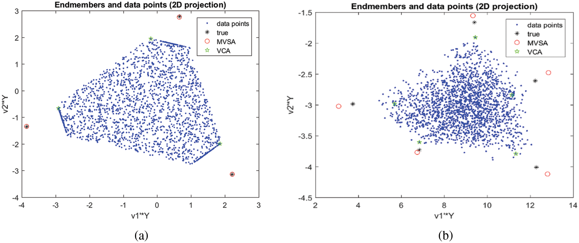
Figure 1: Unmixing results for p = 3, number of endmembers, N = 2000, SNR = 50 and signature type = 3 for NMVF and VCA algorithm. The spectral vectors are represented by dots; with the unmixing algorithm, all other symbols represent inferred endmembers. Notice que quality of NMVF estimates (b) Unmixing results for p = 5, number of endmembers, N = 2000, SNR = 30 and signature type = 1 for NMVF and VCA algorithm

NMVF is exploited to attain an overestimate of the signal subspace. R-CoNMF can be exploited in two ways: (1) to determine the signal subspace, hence including its dimension; or (2) to regulate the subspace of a specified order, provided as input, that reduces the signal prediction fault. In this article, R-CoNMF is exploiteed in the latter way, that is, to evaluate a specified dimension of motion subspace, which does not essentially relate to the number of endmembers in the data. The purpose for this choice is that it frequently happens that the estimate of the correct subspace is a relatively stimulating delinquent owing to, e.g., poor estimate of the noise data or the existence of nonlinear constituents in the data set. Nevertheless, the estimate of an overrate of the signal subspace is an easier delinquent. Therefore, we contribute a value of the estimation variable greater than that determined by NMVF and let R-CoNMF calculate an improved assessment, as it has builtin data related with the LMM not explored in most signal subspace assessment approaches, such as VCA [21], MVSA [22], NMF-MVT [23] and R-CoNMF [24].

Fig. 2 illustrates the numerous outcomes of unmixing for varied endmembers, SNR, and signature type. In Fig. 2a the outcomes of unmixing are defined for p = 3 wherein the number of endmembers denoted by N = 10000 and the SNR considered is 50 and the signature type is 3 for NMVF and VCA algorithm. The spectral vectors are epitomized by dots; with the unmixing procedure, all other symbols signify inferred endmembers. Similarly, Fig. 2b denotes the outcomes of unmixing for p = 10 wherein the number of endmembers denoted by N = 2000 and the SNR considered is 50 and the signature type is 3 for NMVF and VCA algorithm.

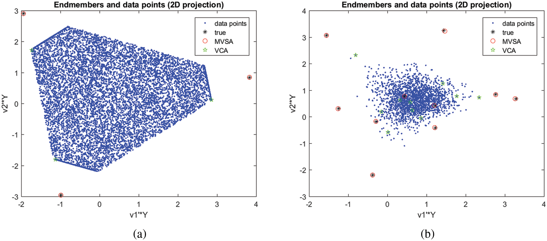
Figure 2: (a) Unmixing results for p = 3, number of endmembers, N = 10000, SNR = 50 and signature type = 3 for NMVF and VCA algorithm. The spectral vectors are represented by dots; with the unmixing algorithm, all other symbols represent inferred endmembers. Notice que quality of NMVF estimates (b) Unmixing results for p = 10, number of endmembers, N = 2000, SNR = 50 and signature type = 3 for NMVF and VCA algorithm

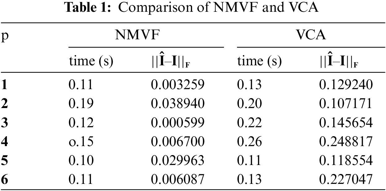
Tab. 1 illustrates the differentiation of NMVF and VCA for the divergent quantity of endmembers wherein the size of the sample is depicted by n whose value is 6000 and || ʥ ||F depicts Frobenius norm of matrix A. In Tab. 1 the time is used and for Frobenius norm || Î – I||F the endmember matrix is estimated yielded by the NMVF and VCA algorithms. The performance of NMVF over VCA is much better concerning error and time. For illustrative purposes, NMVF and VCA algorithms are compared graphically in Fig. 1 that uses simulation run with pixels of non-pure form.

In Fig. 3a the outcomes of unmixing for p = 3, number of endmembers = 2000, SNR = 20 and signature type = 3 for NMVF and VCA algorithm and Fig. 3b illustrates the outcomes of unmixing for p = 5, number of endmembers, N = 2000, SNR = 50 and signature type = 1 for NMVF and VCA algorithm. In Figs. 4a, 4b, it is concluded that when q < p, the inaccuracy of reconstruction is large, and when w ≥ p, the inaccuracy of reconstruction declines significantly, being analogous to the noise level ε. Hence, the correct count of endmembers is easy after the analysis of the turning point of the error of reconstruction. Hence the comparative plot indicates the capability of the proposed method to yield better results than other well-known methods of unmixing.

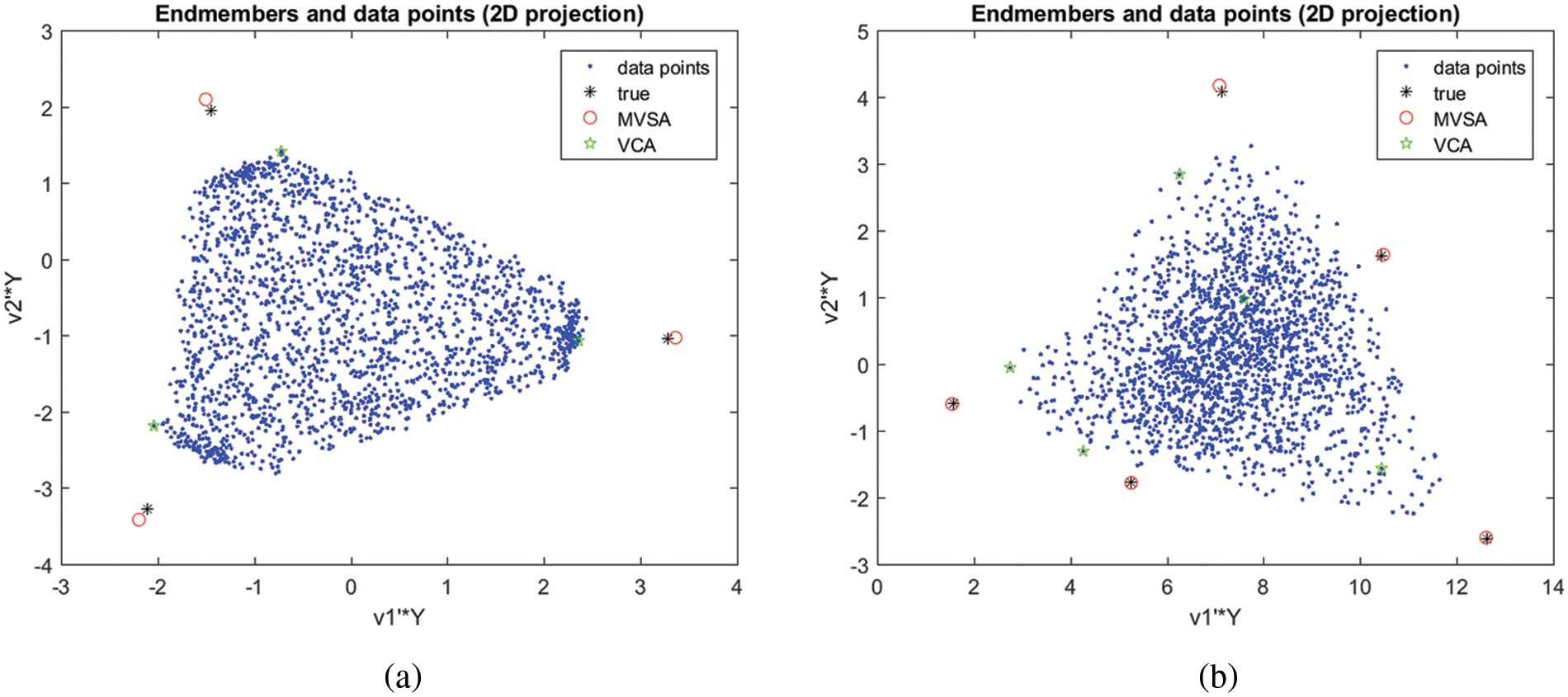
Figure 3: (a) Unmixing results for p = 3, number of endmembers, N = 2000, SNR = 20 and signature type = 3 for NMVF and VCA algorithm. The spectral vectors are represented by dots; with the unmixing algorithm, all other symbols represent inferred endmembers. Notice que quality of NMVF estimates (b) Unmixing results for p = 5, number of endmembers, N = 2000, SNR = 50 and signature type = 1 for NMVF and VCA algorithm

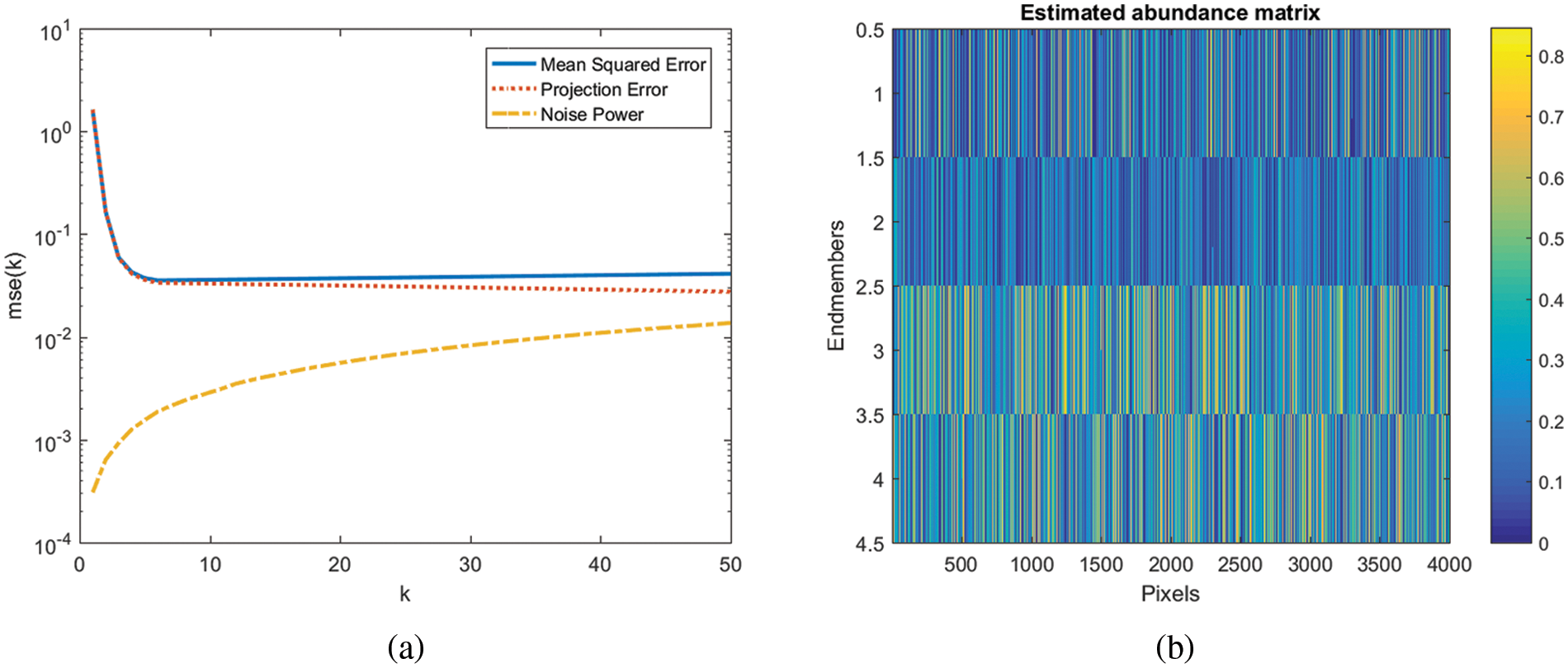
Figure 4: Simulated problem with the value of p = 6, n = 4000, and zero-mean Gaussian i.i.d. noise with SNR = 30 dB. For the dimensions regularizer, we practice the VCA elucidation as its edge. (a) Plot of signal subspace dimension and mse (b) Estimated abundance matrix plot

Tab. 2 provides performance evaluation of R-CoNMF and NMVF to unmix Synthetic data set of HSIs. Cuprite is the supreme standard data customary for the HSI separation examination that explores the Cuprite in Las Vegas, NV, U.S. There are 224 conduits, extending from 368 to 2478 nm.

4.4 Discussion

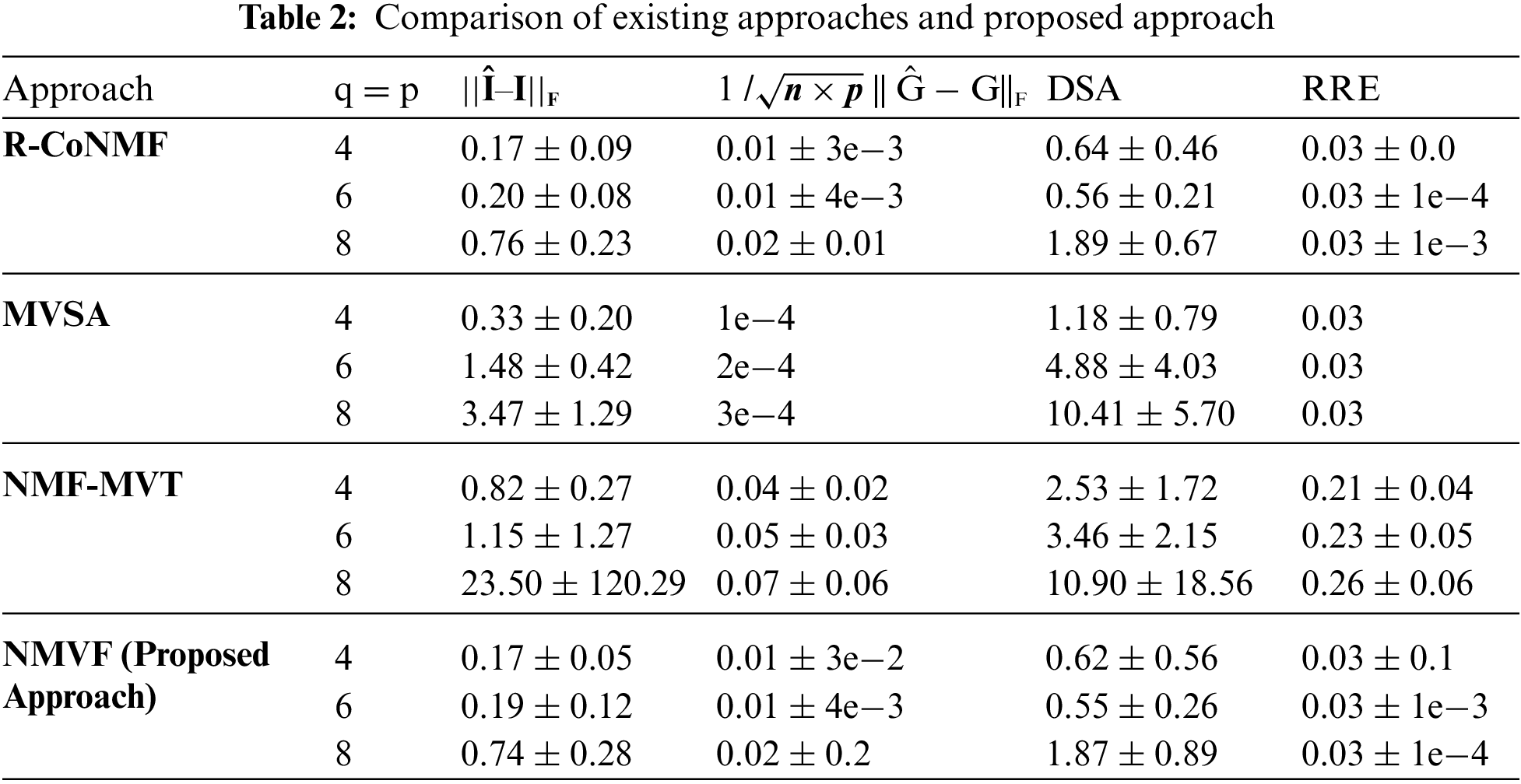
Existing algorithms focus on estimating the EMs count in a section, discerning of spectral signs of EMs, plus approximation of fractional profusion for every EM in every pixel of a scene. Nevertheless, all the stages are performed by only a few algorithms in the process of hyperspectral unmixing. Within the chain, for avoiding the propagation of errors, an efficient technique is highly desirable. The non-negative minimum volume factorization (NMVF) method yields better performance compared to pure pixel-based algorithm. The major approaches are used for comparison that includes VCA [21], MVSA [22], NMF-MVT [23] and R-CoNMF [24]. VCA is an endmember abstraction processes that espouses the postulation of presence of pure constituents i.e., constituents that are copiously donated by a solitary endmember in the experiential data customary. Nevertheless, for the instance of extremely assorted information, the pure-pixel supposition may be totally violated [25]. MVSA is categorized by its higher computational intricacy and comprises a hard constraint in order to make it weak to noise as well as outliers. NMF-MVT was initially anticipated for object acknowledgement and has been lately functional to HSI unmixing. Nevertheless, NMF-MVT may agonize from a non-exclusive decomposition delinquent and can be computationally inflexible when handling huge experimental pixels [26]. The intricacy of the process can be great for circumstances with a huge number of endmembers. Additional drawback is that more comprehensive analysis is necessary for the enactment of the process in extremely assorted circumstances. To offer an additional consistent decomposition in HSI unmixing, NMVF has been anticipated. NMVF initiates with an elementary of huge measurements and then accurately transfers the aspects of the elementary into the information cloud [27–37]. Preferably, NMVF explores additional prior statistics contrasting NMF-MVT. When the integer of endmembers is trivial, i.e., p < 12, NMVF delivers very noble enactment unlike R-CoNMF. Fig. 5 illustrates the spectral signatures obtained by exhausting diverse sets of β, wherein P is delivered by VCA in Fig. 5a and P is demarcated by the data frame in Fig. 5b.

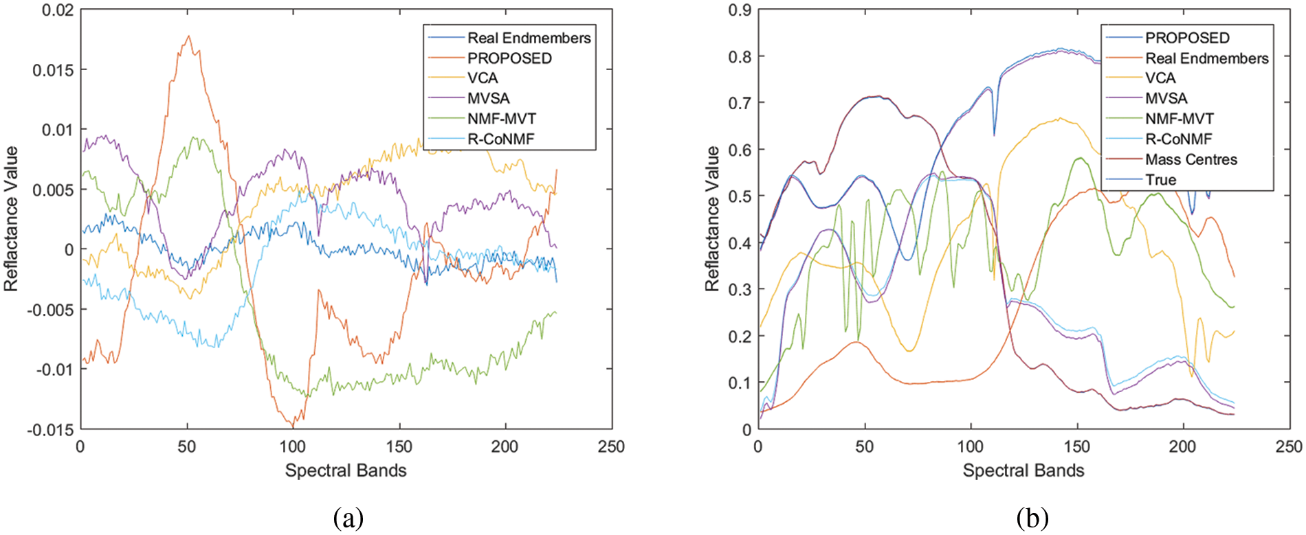
Figure 5: Acquired spectral signatures by expending diverse sets of β. (a) P is delivered by VCA. (b) P is demarcated by the data frame

5  Conclusions and Future Directions

In this research work, spectral unmixing is used to exploit the remotely distinguished HSI data. It identifies a customary of signatures of pure spectra called end members as well as their corresponding fractional, draft rules abundances for every pixel that is captured in HSI. NMVF performs the three major phases of spectral separation sequence: (1) to estimate the count of EMs; (2) to identify a signature of spectra for every EM, and (3) to estimate equivalent profusions for every constituent in the section. A good estimate is provided by the proposed approach for the count of EMs where the information is unavailable a priori and EM signatures of high-quality are generated with abundance estimation even in scenarios with poor visibility.

However, there are few issues presenting challenges over time. For hyperspectral unmixing NMVF hysterics a minutest dimension elementary to the statistics of HSI that restricts the profusion segments be appropriate to the likelihood elementary. The resulting problem of enhancement is then resolved by the implementation of a series of subproblems that are controlled quadratically. The hard constraint in the final step for the profusion fraction is then swapped with a hinge kind loss utility that accounts for outliners and noise. Also, another aspect resolved is the greater comprehensive exploration of the algorithm enactment in decidedly assorted situations such that the present drift for the Earth scrutiny tasks providing greater coverage of the Earth’s surface, leading to coarser spatial resolutions. The NMVF is dominant where unsupervised hyperspectral unmixing is needed and can be efficiently implemented using the interior point method. It also supports other methods like R-CoNMF, where endmember extraction does not require pure pixel presence in the hyperspectral data. Experiment analysis has proved that the proposed approach outperforms existing techniques such as VCA, MVSA, and NMF-MVT. Although the testified dispensation intervals epitomize a very important enhancement concerning the previously existing applications of the process, in impending work we will continue discovering other approaches for enhancement, for instance excruciating the novel HSI into sub-imageries and smearing the manifold-GPU employment respectively. Also, a soft constraint can be included in the anticipated process to craft it further vigorous to noise besides outliers. Besides, the process can likewise be altered to abstract EM packets and hence addressing concerns of EM unevenness.

Ethical Approval: This article does not contain any studies with human participants or animals performed by any of the authors.

Funding Statement: This research was supported by Korea Institute for Advancement of Technology (KIAT) grant funded by the Korea Government (MOTIE) (P0012724, The Competency Development Program for Industry Specialist) and the Soonchunhyang University Research Fund.

Conflicts of Interest: The authors declare that they have no conflicts of interest to report regarding the present study.

1http://lesun.weebly.com/hyperspectral-data-set.html

References

 1.  M. Zhao, L. Yan and J. Chen, “LSTM-DNN based autoencoder network for nonlinear hyperspectral image unmixing,” IEEE Journal of Selected Topics in Signal Processing, vol. 15, no. 2, pp. 295–309, 2021. [Google Scholar]

 2.  K. Kriti and U. Garg, “Unfolding the restrained encountered in hyperspectral images,” International Journal of Recent Technology and Engineering (IJRTE), vol. 8, no. 3, pp. 1023–1038, 2019. [Google Scholar]

 3.  X. Xu, J. Li, S. Li and A. Plaza, “Generalized morphological component analysis for hyperspectral unmixing,” IEEE Transactions on Geoscience and Remote Sensing, vol. 58, no. 4, pp. 2817–2832, 2020. [Google Scholar]

 4.  K. Mahajan, U. Garg and M. Shabaz, “CPIDM: A clustering-based profound iterating deep learning model for HIS segmentation,” Wireless Communications and Mobile Computing, vol. 2021, pp. 1–12, 2021. [Google Scholar]

 5.  M. Zhao, J. Chen and Z. He, “A laboratory-created dataset with ground truth for hyperspectral unmixing evaluation,” IEEE Journal of Selected Topics in Applied Earth Observations and Remote Sensing, vol. 12, no. 7, pp. 2170–2183, 2019. [Google Scholar]

 6.  B. Feng and J. Wang, “Constrained nonnegative tensor factorization for spectral unmixing of hyperspectral images: A case study of urban impervious surface extraction,” IEEE Geoscience and Remote Sensing Letters, vol. 16, no. 4, pp. 583–587, 2019. [Google Scholar]

 7.  K. Kriti and U. Garg, “A comprehensive review of HSI in diverse research domains,” Materials Today: Proceedings, vol. 11, no. 3, pp. 1–15, 2021. [Google Scholar]

 8.  C. A. T. Romero, J. H. Ortiz, O. I. Khalaf and W. M. Ortega, “Software architecture for planning educational scenarios by applying an agile methodology,” International Journal of Emerging Technologies in Learning, vol. 16, no. 8, pp. 132–144, 2021. [Google Scholar]

 9.  L. Qi, J. Li, Y. Wang, Y. Huang and X. Gao, “Spectral-spatial-weighted multiview collaborative sparse unmixing for hyperspectral images,” IEEE Transactions on Geoscience and Remote Sensing, vol. 58, no. 12, pp. 8766–8779, 2020. [Google Scholar]

10. O. I. Khalaf, M. Sokiyna, Y. Alotaibi, A. Alsufyani and S. Alghamdi, “Web attack detection using the input validation method: DPDA theory,” Computers, Materials & Continua, vol. 68, no. 3, pp. 3167–3184, 2021. [Google Scholar]

11. K. Kriti and U. Garg, “Modified silhouette based segmentation outperforming in the presence of intensity inhomogeneity in the hyperspectral images,” International Journal of Intelligent Engineering Informatics, vol. 9, no. 3, pp. 260–275, 2021. [Google Scholar]

12. O. I. Khalaf, “Preface: Smart solutions in mathematical engineering and sciences theory,” Mathematics in Engineering, Science and Aerospace, vol. 12, no. 1, pp. 1–4, 2021. [Google Scholar]

13. M. Berman, H. Kiiveri, R. Lagerstrom, A. Ernst, R. Dunne et al., “ICE: A statistical approach to identifying endmembers in hyperspectral images,” IEEE Transactions on Geoscience and Remote Sensing, vol. 42, no. 10, pp. 2085–2095, 2004. [Google Scholar]

14. X. Ma, X. Zhang, X. Tang, H. Zhou and L. Jiao, “Hyperspectral anomaly detection based on low-rank representation with data-driven projection and dictionary construction,” IEEE Journal of Selected Topics in Applied Earth Observations and Remote Sensing, vol. 13, no. 4, pp. 2226–2239, 2020. [Google Scholar]

15. B. Praveen and V. Menon, “Study of spatial-spectral feature extraction frameworks with 3-D convolutional neural network for robust hyperspectral imagery classification,” IEEE Journal of Selected Topics in Applied Earth Observations and Remote Sensing, vol. 14, no. 3, pp. 1717–1727, 2021. [Google Scholar]

16. M. A. Haq, M. Alshehri, G. Rahaman, A. Ghosh, P. Baral et al., “Snow and glacial feature identification using hyperion dataset and machine learning algorithms,” Arabian Journal of Geosciences, vol. 14, no. 15, pp. 1–21, 2021. [Google Scholar]

17. M. A. Haq, P. Baral, S. Yaragal and G. Rahaman, “Assessment of trends of land surface vegetation distribution, snow cover and temperature over entire Himachal Pradesh using MODIS datasets,” Natural Resource Modeling, vol. 33, no. 2, pp. 1–14, 2020. [Google Scholar]

18. M. A. Haq, G. Rahaman, P. Baral and A. Ghosh, “Deep learning based supervised image classification using UAV images for forest areas classification,” Journal of Indian Society of Remote Sensing, vol. 49, no. 3, pp. 601–606, 2021. [Google Scholar]

19. B. Praveen and V. Menon, “Study of spatial-spectral feature extraction frameworks with 3-D convolutional neural network for robust hyperspectral imagery classification,” IEEE Journal of Selected Topics in Applied Earth Observations and Remote Sensing, vol. 14, no. 2, pp. 1717–1727, 2021. [Google Scholar]

20. X. Zhou, Y. Zhang, J. Zhang and S. Shi, “Alternating direction iterative nonnegative matrix factorization unmixing for multispectral and hyperspectral data fusion,” IEEE Journal of Selected Topics in Applied Earth Observations and Remote Sensing, vol. 13, no. 1, pp. 5223–5232, 2020. [Google Scholar]

21. S. Zhang, A. Agathos and J. Li, “Robust minimum volume simplex analysis for hyperspectral unmixing,” IEEE Transactions on Geoscience and Remote Sensing, vol. 55, no. 11, pp. 6431–6439, 2017. [Google Scholar]

22. T. Chan, C. Chi, Y. Huang and W. Ma, “A convex analysis-based minimum-volume enclosing simplex algorithm for hyperspectral unmixing,” IEEE Transactions on Signal Processing, vol. 57, no. 11, pp. 4418–4432, 2009. [Google Scholar]

23. J. Li, J. M. B. Dias, A. Plaza and L. Liu, “Robust collaborative nonnegative matrix factorization for hyperspectral unmixing,” IEEE Transactions on Geoscience and Remote Sensing, vol. 54, no. 10, pp. 6076–6090, 2016. [Google Scholar]

24. J. Li, A. Agathos, D. Zaharie, J. M. B. Dias, A. Plaza et al., “Minimum volume simplex analysis: A fast algorithm for linear hyperspectral unmixing,” IEEE Transactions on Geoscience and Remote Sensing, vol. 53, no. 9, pp. 5067–5082, 2015. [Google Scholar]

25. B. Goyal, A. Dogra, J. S. Chohan and A. Gupta, “Concurrent clinical optoacoustic and ultrasound imaging for mapping of breast tumor,” Materials Today: Proceedings, vol. 48, pp. 1451–1454, 2022. [Google Scholar]

26. J. S. Chohan, N. Mittal, R. Kumar, S. Singh, S. Sharma et al., “Optimization of FFF process parameters by naked mole-rat algorithms with enhanced exploration and exploitation capabilities,” Polymers, vol. 13, no. 11, pp. 1702, 2021. [Google Scholar]

27. H. Wang, W. Yang and N. Guan, “Cauchy sparse NMF with manifold regularization: A robust method for hyperspectral unmixing,” Knowledge-Based Systems, vol. 184, no. 2, pp. 104898, 2019. [Google Scholar]

28. F. Xiong, Y. Qian, J. Zhou and Y. Y. Tang, “Hyperspectral unmixing via total variation regularized nonnegative tensor factorization,” IEEE Transactions on Geoscience and Remote Sensing, vol. 57, no. 4, pp. 2341–2357, 2018. [Google Scholar]

29. X. R. Zhang, W. F. Zhang, W. Sun, X. M. Sun and S. K. Jha, “A robust 3-D medical watermarking based on wavelet transform for data protection,” Computer Systems Science & Engineering, vol. 41, no. 3, pp. 1043–1056, 2022. [Google Scholar]

30. X. R. Zhang, X. Sun, X. M. Sun, W. Sun and S. K. Jha, “Robust reversible audio watermarking scheme for telemedicine and privacy protection,” Computers, Materials & Continua, vol. 71, no. 2, pp. 3035–3050, 2022. [Google Scholar]

31. M. Abouhawwash and A. Alessio, “Multi-objective evolutionary algorithm for PET image reconstruction: Concept,” IEEE Transactions on Medical Imaging, vol. 12, no. 4, pp. 1–10, 2021. [Google Scholar]

32. M. A. Basset, R. Mohamed, M. Abouhawwash, R. K. Chakrabortty and M. J. Ryan, “EA MSCA: An effective energy-aware multi-objective modified sine-cosine algorithm for real-time task scheduling in multiprocessor systems: Methods and analysis,” Expert Systems with Applications, vol. 173, no. 3, pp. 114699, 2021. [Google Scholar]

33. M. Abouhawwash, “Hybrid evolutionary multi-objective optimization algorithm for helping multi-criterion decision makers,” International Journal of Management Science and Engineering Management, vol. 16, no. 2, pp. 94–106, 2021. [Google Scholar]

34. M. A. Basset, D. Elshahat, K. Deb and M. Abouhawwash, “Energy aware whale optimization algorithm for real-time task scheduling in multiprocessor systems,” Applied Soft Computing, vol. 93, no. 2, pp. 106349, 2020. [Google Scholar]

35. M. Abouhawwash, K. Deb and A. Alessio, “Exploration of multi-objective optimization with genetic algorithms for PET image reconstruction,” Journal of Nuclear Medicine, vol. 61, no. 4, pp. 572, 2020. [Google Scholar]

36. S. Mahajan, A. Raina, M. Abouhawwash, X. Gao and A. K. Pandit, “COVID-19 detection from chest X-Ray images using advanced deep learning techniques,” Computers, Materials and Continua, vol. 70, no. 1, pp. 1541–1556, 2022. [Google Scholar]

37. V. Kandasamy, P. Trojovský, F. Machot, K. Kyamakya, N. Bacanin et al., “Sentimental analysis of COVID-19 related messages in social networks by involving an N-gram stacked autoencoder integrated in an ensemble learning scheme,” Sensors, vol. 21, no. 22, pp. 7582, 2021. [Google Scholar]

This work is licensed under a Creative Commons Attribution 4.0 International License, which permits unrestricted use, distribution, and reproduction in any medium, provided the original work is properly cited.