Computers, Materials & Continua DOI:10.32604/cmc.2022.028942
Article

A Novel Metaheuristic Algorithm: The Team Competition and Cooperation Optimization Algorithm

Tao Wu1, Xinyu Wu1, Jingjue Chen1, Xi Chen2,* and Amir Homayoon Ashrafzadeh3

1School of Computer Science, Chengdu University of Information Technology, Chengdu, 610225, China
2School of Computer Science and Engineering, Southwest Minzu University, Chengdu, 610041, China
3CSIT Department, School of Science, RMIT University, Melbourne, 3058, Australia
*Corresponding Author: Xi Chen. Email: cx@swun.edu.cn
Received: 21 February 2022; Accepted: 07 April 2022

Abstract: Metaheuristic algorithm is a generalization of heuristic algorithm that can be applied to almost all optimization problems. For optimization problems, metaheuristic algorithm is one of the methods to find its optimal solution or approximate solution under limited conditions. Most of the existing metaheuristic algorithms are designed for serial systems. Meanwhile, existing algorithms still have a lot of room for improvement in convergence speed, robustness, and performance. To address these issues, this paper proposes an easily parallelizable metaheuristic optimization algorithm called team competition and cooperation optimization (TCCO) inspired by the process of human team cooperation and competition. The proposed algorithm attempts to mathematically model human team cooperation and competition to promote the optimization process and find an approximate solution as close as possible to the optimal solution under limited conditions. In order to evaluate the performance of the proposed algorithm, this paper compares the solution accuracy and convergence speed of the TCCO algorithm with the Grasshopper Optimization Algorithm (GOA), Seagull Optimization Algorithm (SOA), Whale Optimization Algorithm (WOA) and Sparrow Search Algorithm (SSA). Experiment results of 30 test functions commonly used in the optimization field indicate that, compared with these current advanced metaheuristic algorithms, TCCO has strong competitiveness in both solution accuracy and convergence speed.

Keywords: Optimization; metaheuristic; algorithm

1  Introduction

Metaheuristic algorithm combines the advantages of random search algorithm and local search algorithm. Compared with the optimization algorithm that gives a clear optimal solution, the metaheuristic algorithm gives an optimal solution or approximate solution to the optimization problem under limited conditions. In recent years, traditional optimization algorithms can hardly meet the accuracy requirements of various fields such as engineering, business and economics for optimization problems under limited conditions [1]. Compared with traditional optimization algorithms, metaheuristic algorithms have the following advantages. First, the algorithm is simple and easy to implement [2,3]; second, it requires less time and space, and can be adjusted according to the user's accuracy requirements [4]; third, the algorithm can jump out of the local optimal solution to a certain extent and approach the global optimal solution as close as possible. Generally, the metaheuristic optimization algorithm includes two parts, exploration and exploitation. Due to the randomness of the metaheuristic algorithm, finding a proper balance between these two parts is a challenging task [5].

The No Free Lunch theorem (NFL) [6] shows that there is no metaheuristic algorithm that can solve all optimization problems at the same time. The NFL theorem makes this field of study highly active. It allows researchers to improve existing algorithms or propose new algorithms to better address various optimization problems. In this paper, the experiments show that compared with the latest excellent optimization algorithms, such as Whale Optimization Algorithm (WOA) [7], Sparrow Search Algorithm (SSA) [8], Seagull Optimization Algorithm (SOA) [9], Grasshopper Optimization Algorithm (GOA) [10], TCCO has made significant progress.

The rest of the paper is structured as follows. Section 2 presents a literature review of metaheuristic algorithms. Section 3 presents the details about TCCO and its pseudo-code implementation. Section 4 provides the comparative statistical analysis of results on benchmark functions. Section 5 concludes the work and suggests some directions for future studies.

2  Related Work

In the past few decades, researchers have developed a series of metaheuristic algorithms inspired by nature to solve optimization problems under limited conditions. They can be roughly divided into the following four classes:

The metaheuristic algorithm based on Darwinian theory of evolution. For instance, the Genetic Algorithm (GA) [11] proposed by Holland et al. seeks the optimal solution by imitating the natural selection, genetic and mutation mechanisms in the biological evolution; the Biogeography-Based Optimizer proposed by Simon (BBO) [12], which is inspired by biogeography regarding the migration of species between different habitats, as well as the evolution and extinction of species. These algorithms have been widely used in process control, signal processing, image processing, flexible job shop scheduling, machine learning and other fields. Excellent traits have a greater probability of being inherited, which is one of the main advantages of evolutionary algorithms. Besides, the algorithms are scalable and easy to combine with other algorithms. The disadvantage is that they may fall into a local optimal solution and lead to premature convergence.

The second class is physics-based algorithms. This type of algorithm seeks the optimal solution by imitating the physical rules that are common in the real world. For example, the annealing idea proposed by Metropolis et al. was introduced into the field of optimization problems by Kirkpatrick et al. and designed the simulated annealing algorithm (SA) [13]. Although the simulated annealing algorithm has a simple calculation process, it is universal, and has strong robustness. It can be used to solve complex non-linear problems. But there are also disadvantages such as slow convergence speed, long execution time, performance related to initial values and parameter sensitivity; different from SA, the Gravitational Search Algorithm (GSA) [14] proposed by Esmat et al. is an optimization algorithm based on the law of universal gravitation. It finds the optimal solution by moving the particle position of the population; furthermore, the artificial electric field algorithm (AEFA) [15] designed by Yadav, which is inspired by the Coulomb law, finds optimal solution by simulating the movement of charged particles in an electrostatic field.

Algorithms based on swarm intelligence is the third class, they find the optimal solution by simulating the activities of biological swarms. The Particle Swarm optimization algorithm (PSO) [16] designed by Kennedy et al. It is inspired by the social behavior of a flock of birds. Individuals are abstracted into particles, and all particles have a fitness value determined by a user defined fitness function. Each particle also has a speed that determines the direction and distance of their flight, and then the particles follow the current optimal particle to search in the solution space. The ant colony optimization (ACO) [17] proposed by Dorigo et al. is inspired by the social behavior of ants. In fact, the social intelligence of ants in finding the closest path from the nest and a source of food is the main inspiration of this algorithm. The Whale Optimization Algorithm (WOA) [7] designed by Mirjalili et al., which mimics the hunting behavior of humpback whales. In the WOA algorithm, the position of each humpback whale represents a feasible solution. The sparrow search algorithm (SSA) [8] designed by Xue et al. finds the optimal solution by simulating the strategy of predation and avoiding natural enemies of sparrow groups. This kind of swarm intelligence algorithm also has problems such as easy to fall into local optimal solution and slow convergence speed. The Rock Hyraxes Swarm Optimization (RHSO) [18] designed by Al-Khateeb et al., which mimics the collective behavior of rock hyraxes to find their eating and their special way of looking at this food. RHSO is very effective in solving real issues with constraints.

The Fourth subclass is the algorithms based on human behavior, such as CAs [19] and ICA [20]. In the Cultural Algorithms (CAs) [19], the belief space serves as a knowledge database in which people's past experience is stored, so that future generations can learn from the knowledge. As a result, the evolution speed of the population surpasses the evolution speed of purely relying on biological genetic inheritance, and has good global optimization performance. The Imperialist Competitive Algorithm (ICA) [20] designed by Atashpaz et al. is an optimization method formed by simulating the colony assimilation mechanism and the imperial competition mechanism.

3  The Team Competition and Cooperation Optimization Algorithm

In this section, we will elaborate on the inspiration of TCCO, the mathematical model and pseudo-code.

3.1 Algorithm Inspiration

Competition and cooperation exist everywhere in human society. The development of human society is largely driven by competition and cooperation. Therefore, this paper attempts to mathematically model cooperation and competition to promote the optimization process and find an approximate solution as close as possible to the optimal solution under limited conditions. At the same time, the concept of team and intra-team update in algorithm naturally support parallel computation, the simple and efficient inter-team cooperation also allow the algorithm to be parallelized with a small communication cost. In addition, considering the massive computing power of the parallel system, this algorithm also designs a process of judging the advantage of team members, which improves the performance and convergence speed of the algorithm to a certain extent.

The competition and cooperation process in this paper can be simplified into the following steps. First, people are divided into several teams. In order to achieve a same goal, everyone proposes their own pre-solution to this problem. Each team selects a leader according to the quality of their solution. The cooperation is advanced under the organization of the leader, trying to find a better solution. After all the team members updated their own solution, a new leader is selected, and then the best solution is used to participate in the team competition. The team with the best solution wins and becomes the dominant team. Next, each team randomly finds their own partners to work together to optimize their solution. However, the dominant team has the right to choose more partners than other teams. If your team's solution is better than partner's, they will follow you, otherwise thing reversed. After the cooperation, people of each team should re-elect the leader and participate in the team competition. When all the teams have completed these steps, the current round of competition and cooperation process ends. After multiple rounds of this process, the solution given by the dominant team will become the final solution.

3.2 Mathematical Model and Pseudo-Code Implementation

In order to simplify the mathematical model, this paper is based on the following assumptions:

Assumption 1: Each member is identical except for his own solution.

Assumption 2: Each ordinary team's partner count is partnerNorm, but the dominant team is partnerBest.

Assumption 3: The population is equally divided into teamN teams (teamN>1) and satisfies (teamN−partnerBest−1)  mod (partnerNorm + 1) = 0. Besides, the number of members in each team is bigger than 1(memberN> 1).

Assumption 4: Pre-solution and random grouping are implemented by random initialization.

Assumption 5: The solution is a feasible solution of the objective function, and its quality is measured by the fitness function. This paper defines that the solution with lower fitness value is better.

Assumption 6: When the solution proposed by ordinary members and leaders, ordinary team and dominant team have the same fitness values, the solution of the leader and dominant team is given priority.

Assumption 7: The team leader's solution is defined as the team's solution.

Assumption 8: The process of advantages judgment is simplified to the member replaces the corresponding items of others with their own items in turn. Items are defined as advantages only if the solution is better after be replaced.

In this paper, partnerNorm = 1, partnerBest = 2, the number of team is set to 7 (teamN = 7), the number of team members is also 7 (memberN = 7) and the population size is 49. Fig. 1 shows the basic flow chart of TCCO.

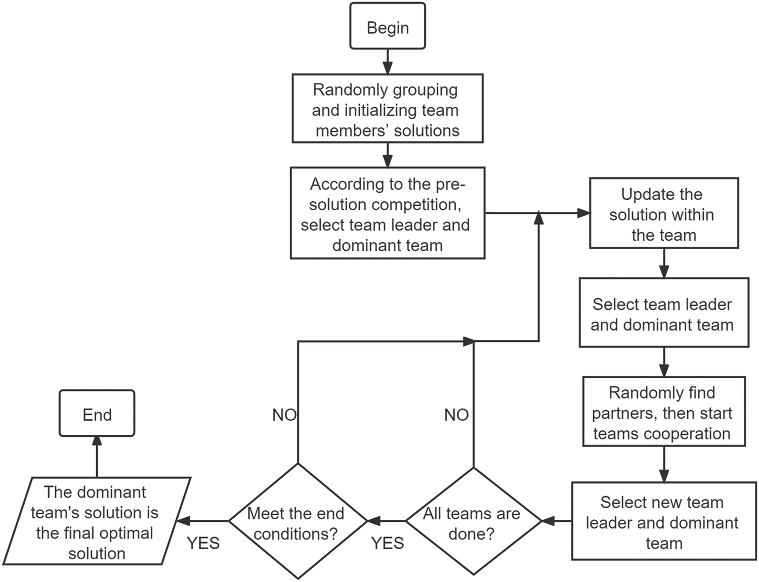
Figure 1: TCCO algorithm flow chart

3.2.1 Grouping and Pre-Solution

There are 7 teams in this paper, and each team contains 7 members. It can be seen from assumptions 1 and 5 that members can be abstracted as feasible solutions, and the members of a team can be specified by a matrix. Each row of the matrix identifies a member. See Eq. (1) for details, where d represents the dimension of the objective function.

Mn=[m1,1m2,1⋮mmemberN,1m1,2m2,2⋮mmemberN,2⋯⋯⋱…m1,dm2,d⋮mmemberN,d](n=0,1,…,teamN−1)(1)

mi=borderL+  uniform(0, 1)∗(borderH−borderL)(2)

Eq. (2) gives the initialization method of each pre-solution, where mi represents a feasible solution, borderL and borderH are lower and upper bounds of objective function. The uniform(0, 1) is a uniformly distributed random d-dimension vector in the range [0, 1].

3.2.2 Fitness Function and Competition

Generally, under the condition of assumption 5, if the objective function f(x) is a maximization problem and its value range is non-negative, then the fitness function Fit(x)=1f(x). If f(x) is a minimization problem, it can be simply mapped to Fit(x)=f(x).

Fit(x)=f(x)(3)

Fit(Mn)=[f(m1,1, m1,2,…,m1,d)f(m2,1, m2,2,…,m2,d)⋮f(mmemberN,1,mmemberN,2,…,mmemberN,d)](4)

leadern= Mn[argmin(Fit(Mn))](5)

leaderV=Fit([leader1,leader2,…,leadern]T)(6)

leaderTeam=Margmin(leaderV)(7)

Eq. (5) gives the selection method of the team leader, where leadern represents the solution of the team leader, that also is, the solution of the team. argmin(x) represents the index of the minimum value of vector x, and the leader of each team follows the assumption 6 responsible by the best solution within the contemporary team. Eq. (7) gives the selection method of the leading team, and the dominant team is also defined as the team with the best solution among all teams according to Assumption 6. The selection of the team leader and the dominant team together constitutes the competition in this algorithm.

3.2.3 Update Solutions within the Team

For ordinary members of the team, they have three ways to update their solution. In this paper, there is a probability Pleader=0.6 that members will follow the team leader. Members in one team can share their solutions without reservation, so that members can learn from leader to improve their own shortcomings, at the same time, the leader also can absorb advantages of their members; besides, there is a probability PdominantTeam=0.3 for all members to follow the leader of the dominant team, in order to surpass the leader of their own team. But because they are not in the same team, they can only learn and improve from the leader of the dominant team in the general direction, and they cannot communicate with each other; furthermore, there is also a probability of 1−Pleader−PleaderTeam=0.1, members can choose not to follow and freely explore their own solutions. In general, the free exploration probability can affect the exploration and exploitation capabilities of the algorithm. The greater the probability, the stronger the exploration ability of the algorithm. errorRange is the following error, which is positively related to the distance between itself and the following target, and is limited by the number of current iteration. As the number of iteration increases, it gradually approaches zero. The expression is given by Eq. (8), where abs is the absolute value function, the tMax is the maximum iteration and the t is current iteration.

errorRange=uniform(0,1)∗(tMax −  t)tMax∗abs(mi−dest)(8)

exploreRange=uniform(0,1)∗(borderH−borderL)∗d∗(tMax −  t)teamN∗memberN∗tMax(9)

1.    Follow the team leader, update method is given in Eq. (15). Ti in Eq. (10) is a real symmetric matrix, the diagonal elements are the elements of the member to be updated, and the remaining elements are the same as the team leader. The weaknessi vector given in Eq. (11) represents the disadvantage items of the member compared to the leader, and the strengthi given in Eq. (12) represents the advantage items. The errorRange and exploreRange are given by Eqs. (8) and (9), in this case, dest is the team leader, and p is a random number in the interval [0, 1] that obeys a uniform distribution.

Ti=[mi,1mleader,1⋮mleader,1mleader,2mi,2⋮mleader,2⋯⋯⋱…mleader,dmleader,d⋮mi,d](10)

weaknessi=Fit(Ti)>fitleader (11)

strengthi=Fit(Ti)≤fitleader(12)

mit+1[dim]={leadernt[dim]+errorRange,  p<0.5leadernt[dim]−errorRange,  p≥0.5(13)

mit+1[dim]={mit[dim]+exploreRange,  p<0.5mit[dim]−exploreRange,  p≥0.5(14)

mit+1={(13),  dim⁡ in weknessi(14),  dim⁡ in strengthi(15)

2.    Follow the leader of the dominant team, the errorRange is given by Eq. (8). In this case, dest is dominant team's leader, and p is a random number in the interval [0, 1] that obeys a uniform distribution.

mit+1={leaderTeamnt+uniform(0,1)∗errorRange,  p<0.5leaderTeamnt−uniform(0,1)∗errorRange,  p≥0.5(16)

3.    Same update method as Eq. (2) for free exploration. mit+1=borderL+  uniform(0, 1)∗(borderH−borderL)

For the team leader, he will learn the advantages of all other members, and Eq. (17) gives the update method. In a word, it is to gather the advantages of his team members.

leadernt+1[dim]=Mn[argmin(Fit([T1[dim],T2[dim],…,TmemberN[dim]))][dim](17)

In particular, for the first and second update methods of the above-mentioned ordinary members, when the feasible solution exceeds the range of the solution space, this paper simply adopts the method of directly taking the boundary value. After a round of update solutions are completed, a new team leader will be selected according to Assumption 6 and Eq. (5), and a new dominant team will be selected according to Assumption 6 and Eq. (7).

3.2.4 Teamwork to Update Solutions

After all members updated, the team randomly search for partners according to Assumption 2. In the two teams that cooperate, all members will follow the better solution. The way to update the solution is given by Eq. (18). Step is the number of times that each team continuously proposes better solutions in all collaborations. In other words, once the team solution is worse than cooperation team, step will be reset to 1. The errorRange is given by Eq. (8), dest is the solution of the better team in this case, and p is a random number with uniform distribution in the interval [0, 1].

mi={dest+step∗errorRange,  p<0.5dest−step∗errorRange,  p≥0.5(18)

When the feasible solution exceeds the solution space, the method of directly taking the boundary value is also simply adopted in this paper. After a round of collaborative update solutions between teams, a new team leader will be selected according to Assumption 6 and Eq. (5), and a new dominant team will be selected according to Assumption 6 and Eq. (7).

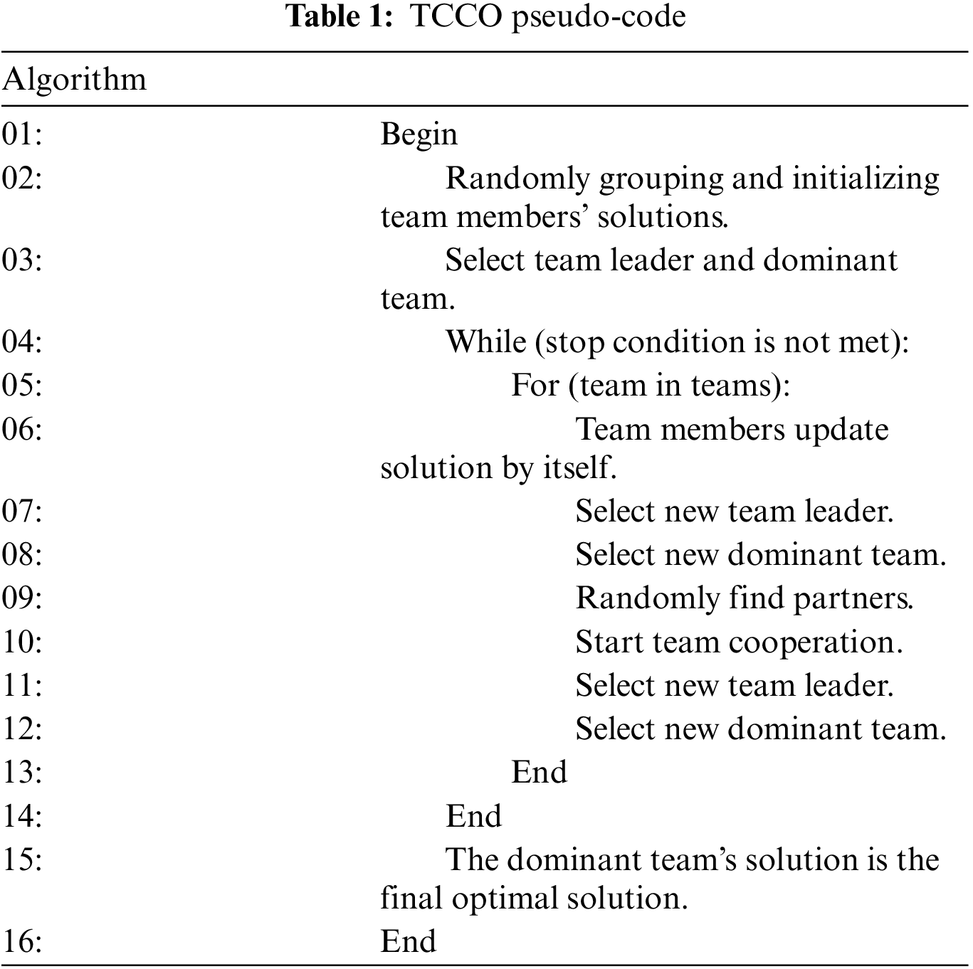
3.2.5 TCCO Pseudo-Code Implementation

Tab. 1 shows the team competition and cooperation optimization algorithm's main pseudo-code.

4  Experiment and Analysis

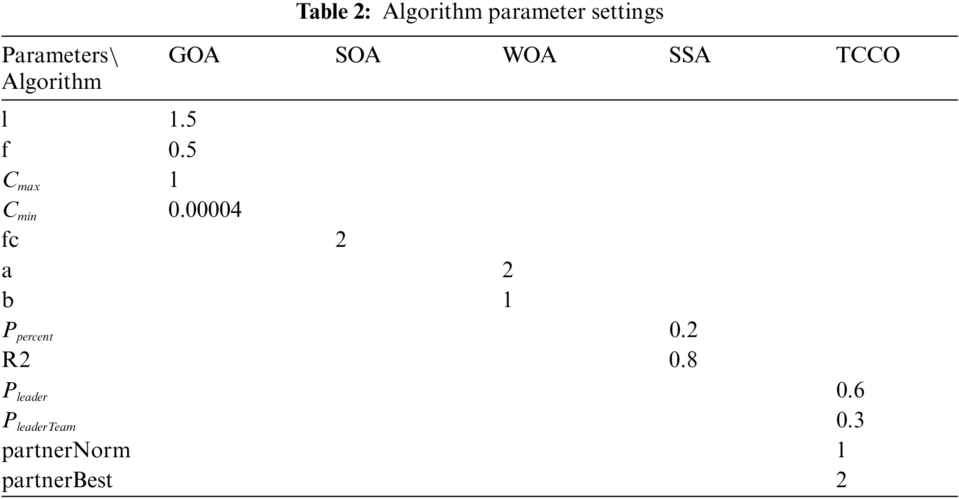
In this section, the TCCO is benchmarked on 30 classic benchmark functions [1,21,22] compared with the Whale Optimization Algorithm (WOA), Sparrow Search Algorithm (SSA), Seagull Optimization Algorithm (SOA) and Grasshopper Optimization Algorithm (GOA) to analysis it's performance. All algorithms are basic version, and the parameter settings are shown in Tab. 2. In this paper, 30 classic benchmark functions are divided into 4 categories: low-dimensional unimodal, low-dimensional multimodal, high-dimensional unimodal, and high-dimensional multimodal according to dimensions and modals. Four sets of experiments are performed to test and compare the performance of the above algorithms. In order to compare the performance fairly, the population size of all algorithms is set to 49, and the maximum number of iterations is 500. At the same time, in order to make the comparison experiment more general, each algorithm will run the benchmark function 30 times to compare the average, best, and worst solutions of 30 classic benchmark functions.

4.1 The Experiments of Low-Dimensional Unimodal Functions

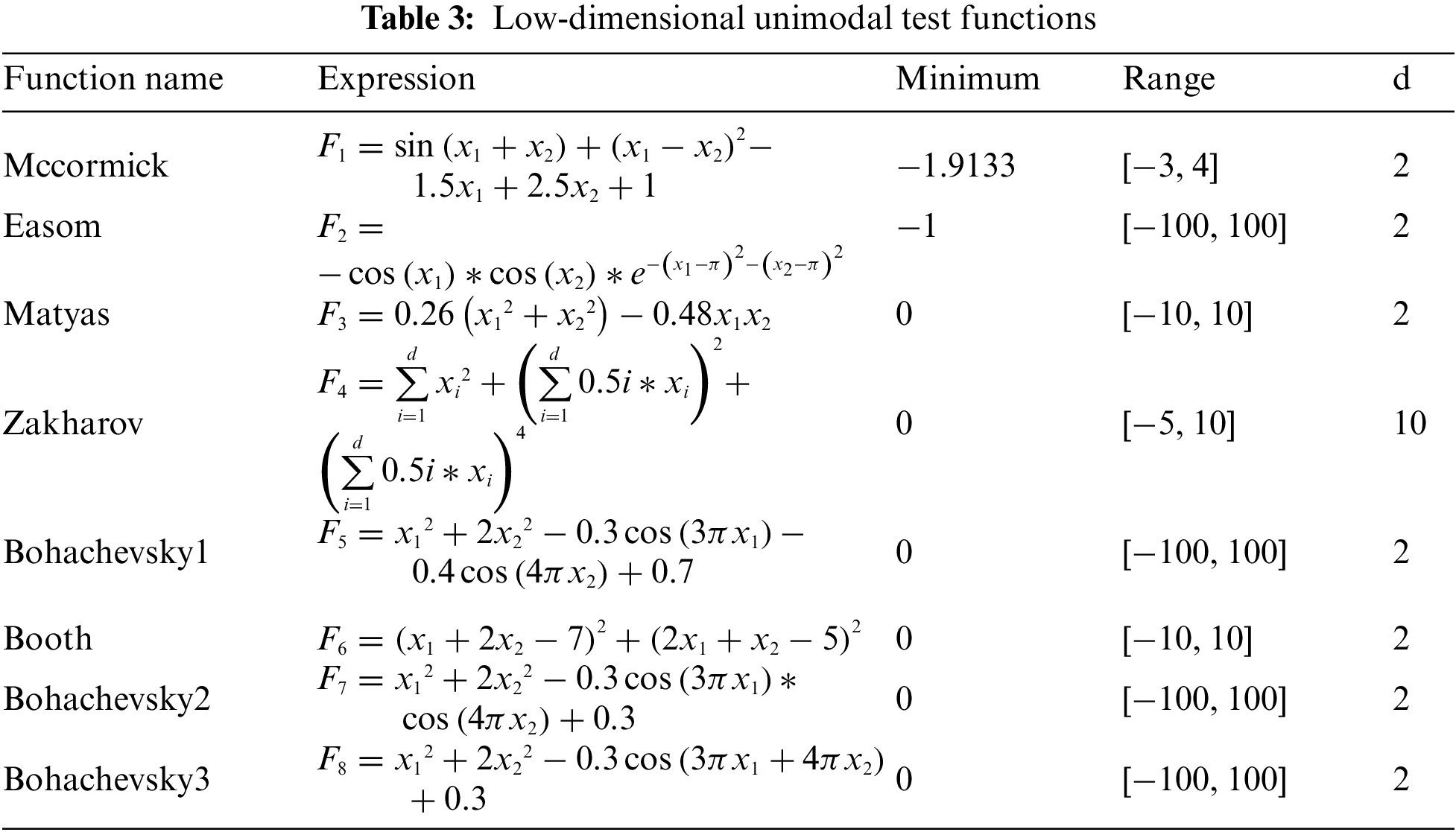
This section will conduct experiments on the first set of eight low-dimensional unimodal test functions to compare the performance of the above five optimization algorithms. The name, expression, minimum value, range and dimension of the functions are shown in Tab. 3.

Tab. 4 shows the experiment results of 8 low-dimensional unimodal test functions and advantages are shown in bold. In the average solution comparison, SOA won 3 items, WOA won 4 items and TCCO won 6 items. In the comparison of minimum values, GOA got 1 item, SOA got 2 items, WOA got 3 items and SSA got 4 items, while TCCO has 7 wins. In the maximum value item, SOA won 3 items, WOA won 4 items and TCCO won 6 items. Fig. 2 shows the convergence performance of each algorithm under eight test functions (run once, maximum iteration set to 20). The results show that TCCO has a slight lead in convergence speed and accuracy.

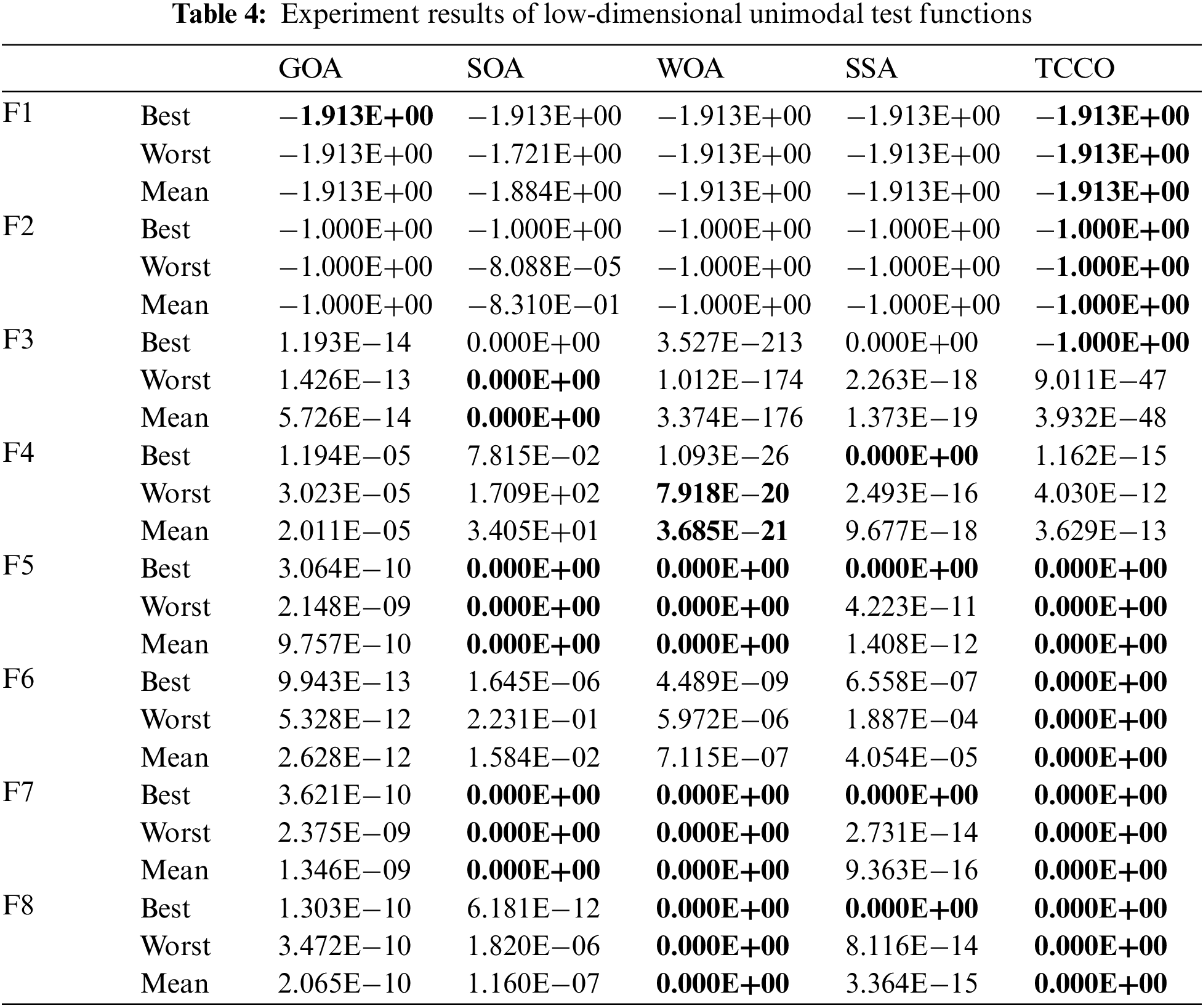
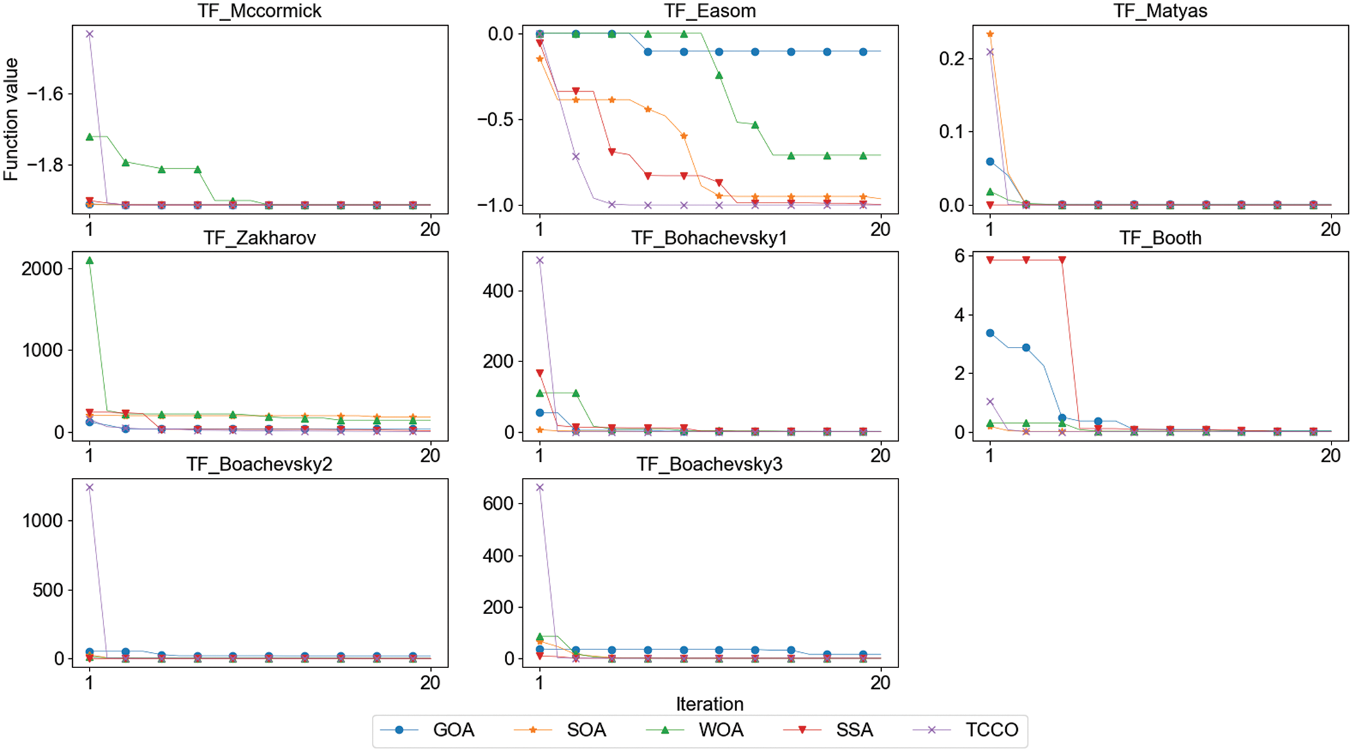
Figure 2: Convergence speed comparison of low-dimensional unimodal test functions

4.2 The Experiments of Low-Dimensional Multimodal Functions

This section will conduct experiments on the second set of 12 low-dimensional multimodal test functions to compare the performance of the above five optimization algorithms. The name, expression, minimum value, range and dimension of the function are shown in Tab. 5, and the results of experiment are shown in Tab. 6. Fig. 3 shows the convergence performance of each algorithm under twelve test functions (run once, maximum iteration set to 20).

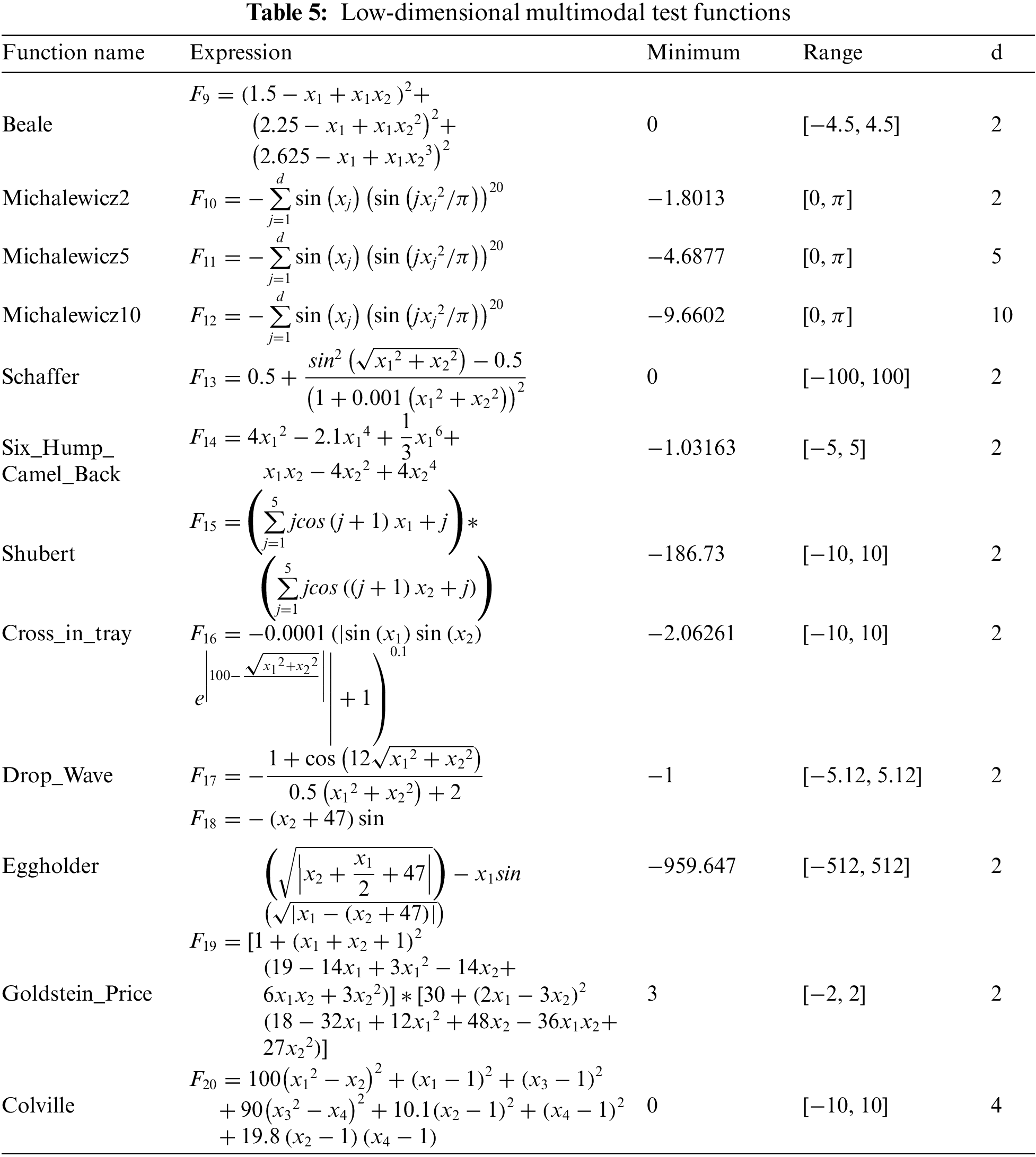
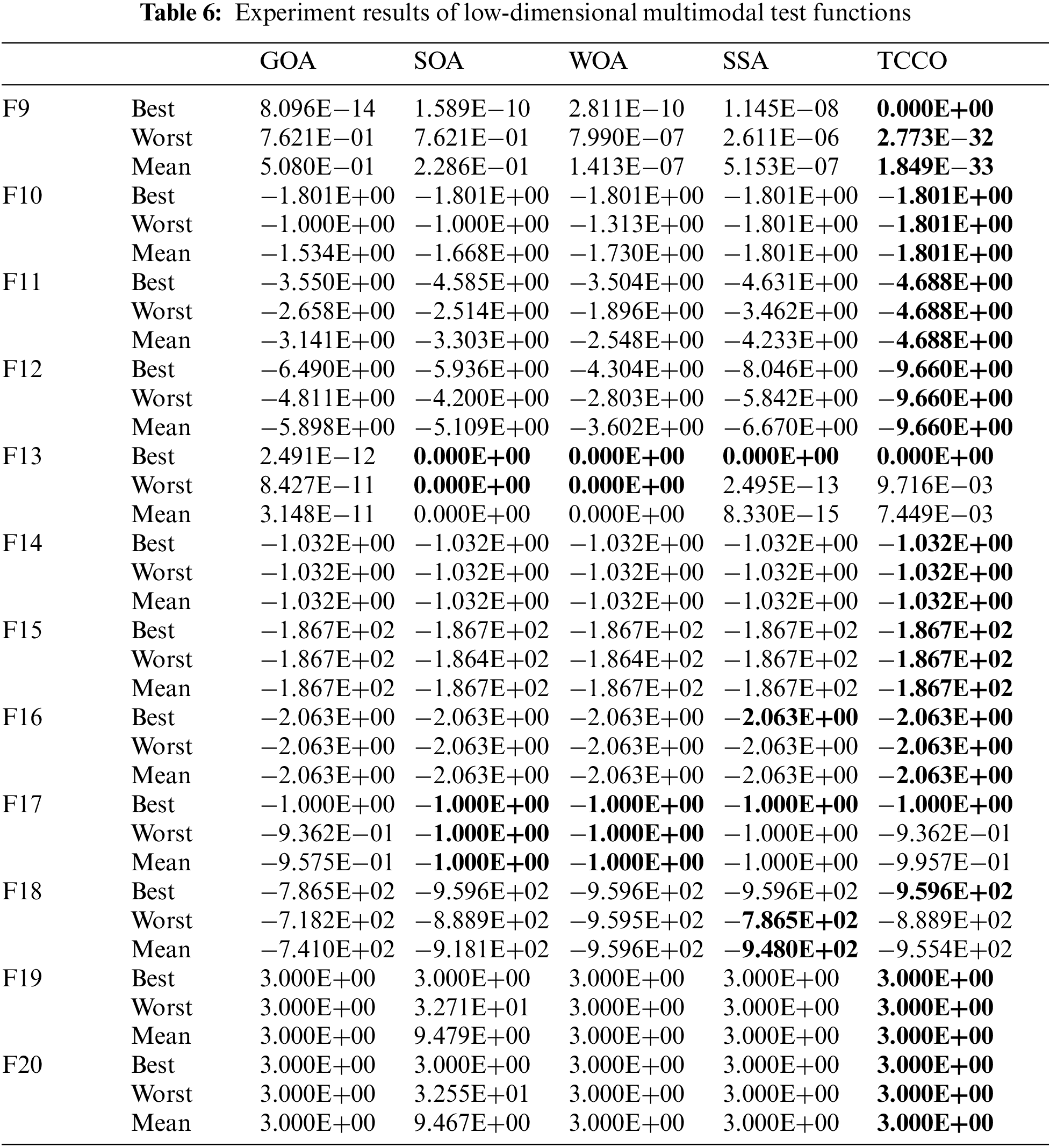
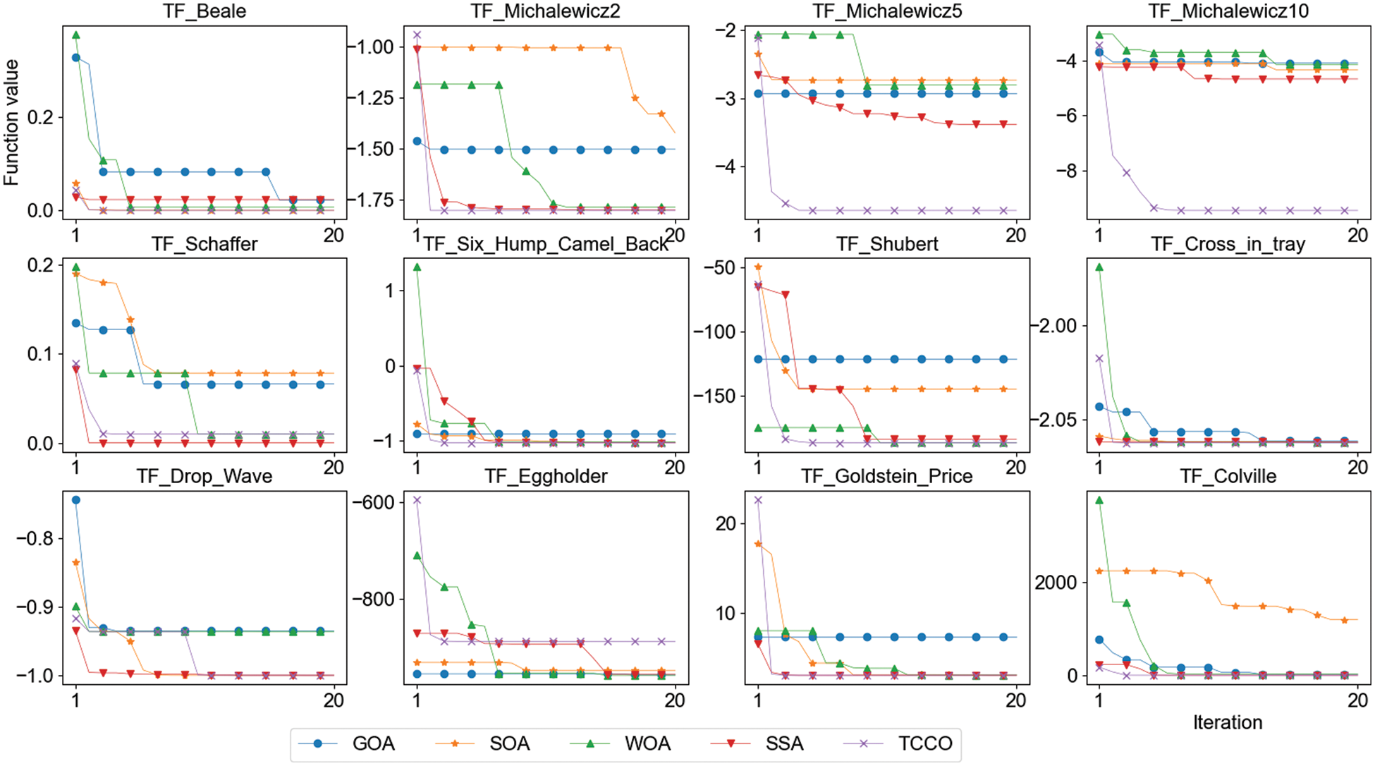
Figure 3: Convergence speed comparison of low-dimensional multimodal test functions

4.3 The Experiments of High-Dimensional Unimodal Functions

This section will conduct experiments on the third group of 7 high-dimensional unimodal test functions to compare the performance of the above 5 optimization algorithms. The name, expression, minimum value, range and dimension of the function are shown in Tab. 7; the results of experiment are shown in Tab. 8. Fig. 4 shows the convergence performance of each algorithm under seven test functions (run once, maximum iteration set to 20).

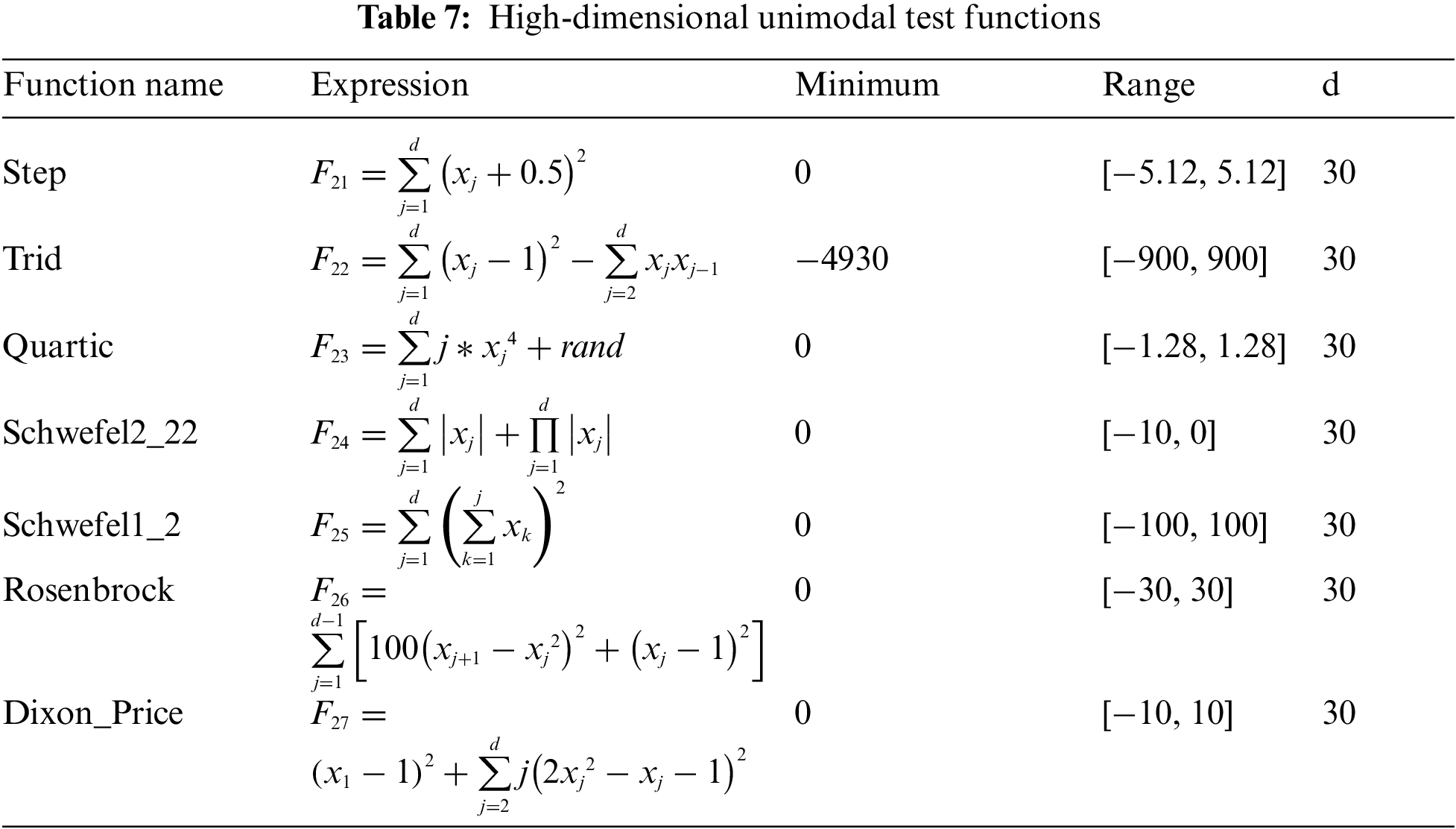
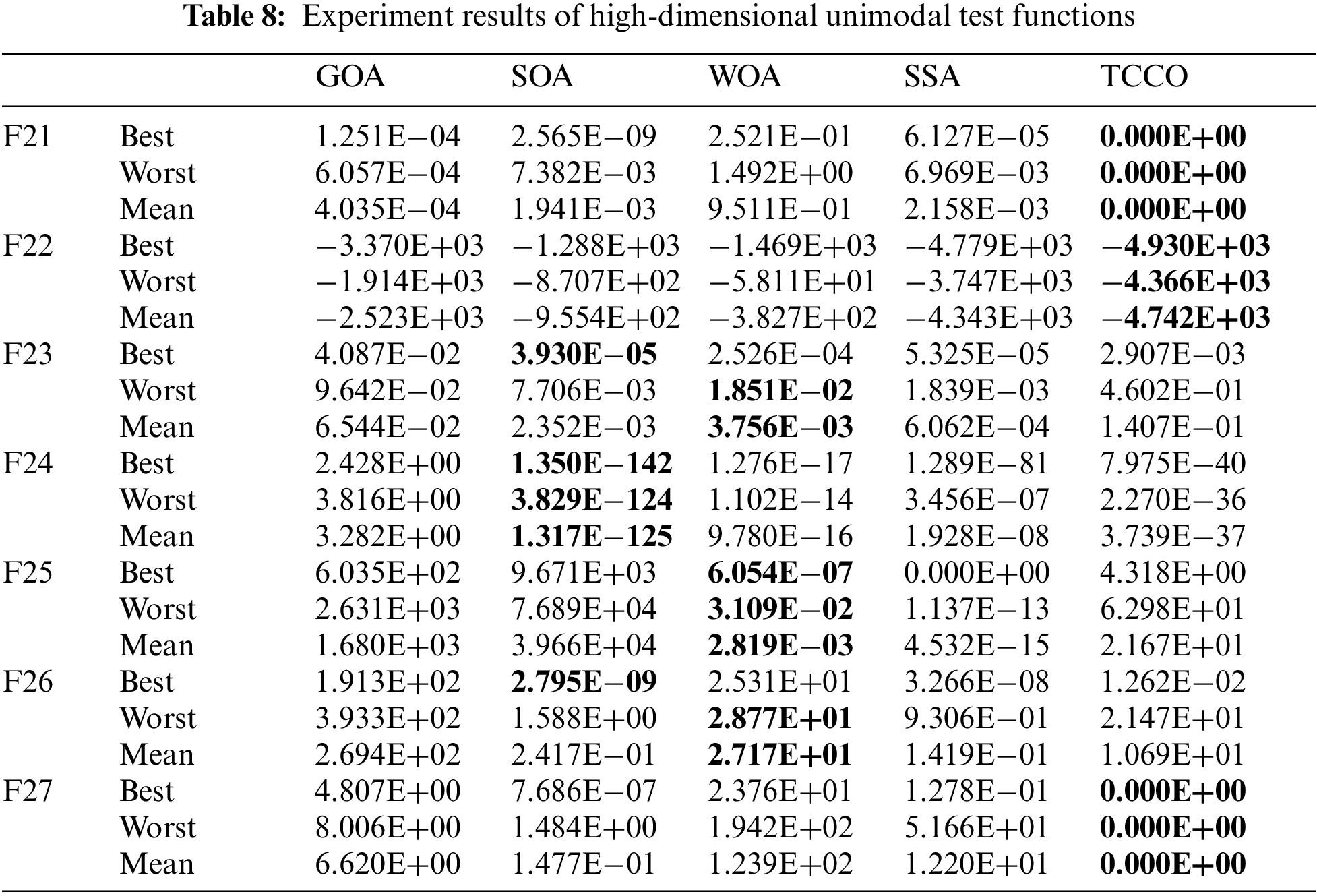
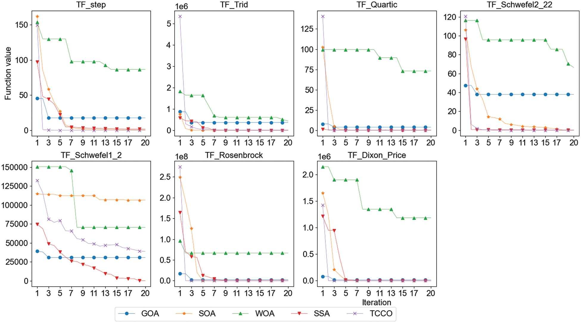
Figure 4: Convergence speed comparison of high-dimensional unimodal test functions

4.4 The Experiments of High-Dimensional Multimodal Functions

This section will conduct experiments on the fourth group of three high-dimensional multimodal test functions to compare the performance of the above five optimization algorithms. The name, expression, minimum value, range and dimension of the function are shown in Tab. 9; the results of experiment are shown in Tab. 10. Fig. 5 shows the convergence performance of each algorithm under three test functions (run once, maximum iteration set to 20).

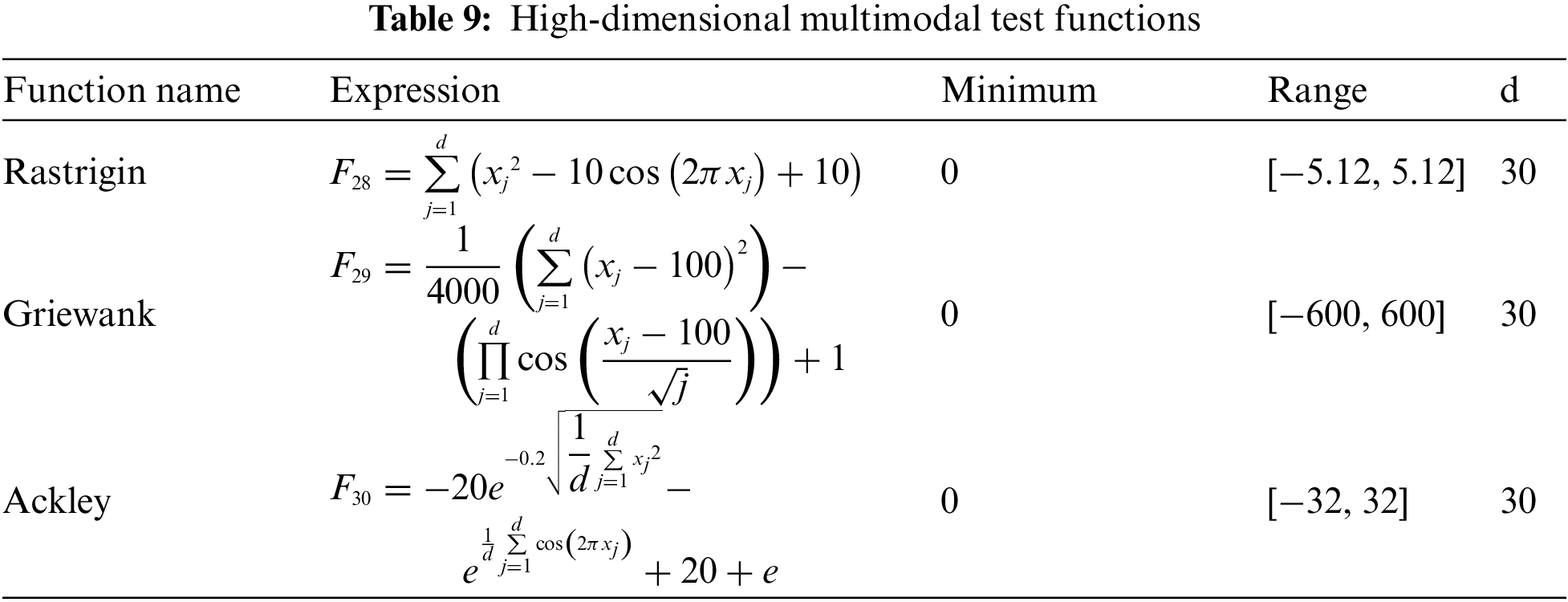
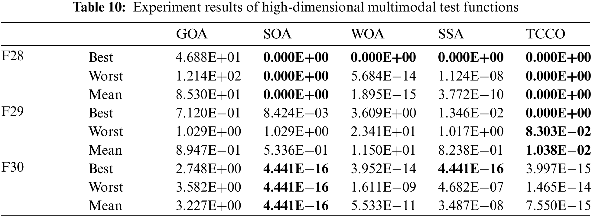
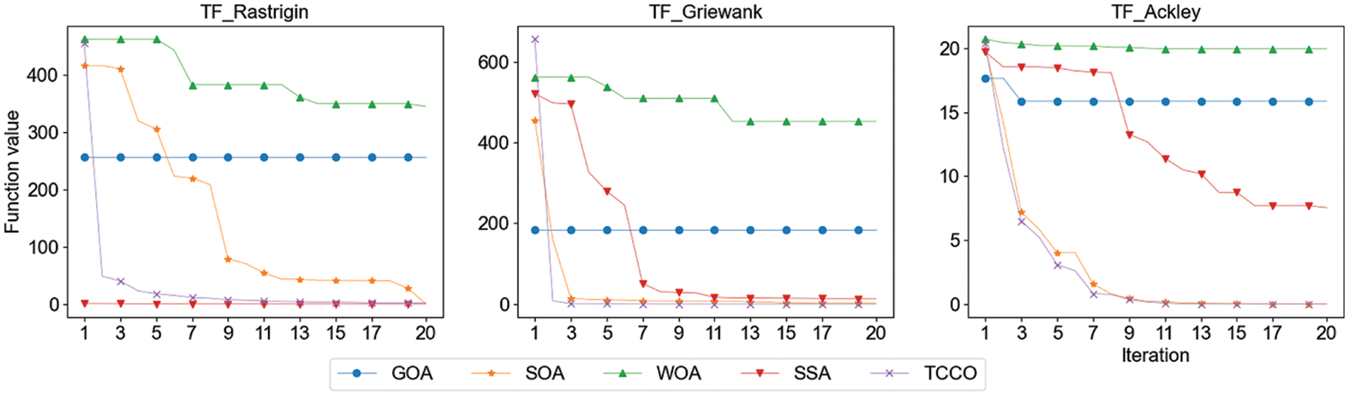
Figure 5: Convergence speed comparison of high-dimensional multimodal test functions

4.5 Analysis of Results

Unimodal function has only one global optimal solution in the solution space. This type of function can well evaluate the exploitation ability of metaheuristic algorithm. Experiment 1 and experiment 3 show that whether it is a low-dimensional unimodal function or a high-dimensional unimodal function, TCCO has good performance compared with other algorithms, and the convergence speed is faster than other algorithms.

Different from unimodal function, multimodal function has many local optimal solutions in the solution space. The number of local optimal solutions increases exponentially with the growth of the problem scale. Therefore, this type of test function is often used to evaluate the exploration capability of metaheuristic algorithm. Experiment 2 and 4 are designed for this purpose. The experiment results show that the performance of TCCO is better than other algorithms in both low-dimensional multimodal function and high-dimensional multimodal function.

5  Conclusion

This research is inspired by the competition and cooperation between human teams, and proposes a new metaheuristic optimization algorithm, Team Competition and Cooperation Optimization Algorithm (TCCO), which is easy to parallelize. TCCO includes two operators, which respectively simulate the update solution within the team and the update solution between teams. This paper conducts detailed experiments on 30 benchmark functions, compared and analyzed the exploration ability, exploitation ability and convergence speed of WOA, SSA, SOA, GOA and TCCO. Experiment results show that compared with other metaheuristic algorithms mentioned above, TCCO has stronger competitiveness.

Funding Statement: This research was partially supported by the National Key Research and Development Program of China (2018YFC1507005), Sichuan Science and Technology Program (2020YFG0189, 22ZDYF3494), China Postdoctoral Science Foundation (2018M643448), and Fundamental Research Funds for the Central Universities, Southwest Minzu University (2022101).

Conflicts of Interest: The authors declare that they have no conflicts of interest to report regarding the present study.

References

 1.  M. Jain, V. Singh and A. Rani, “A novel nature-inspired algorithm for optimization: Squirrel search algorithm,” Swarm and Evolutionary Computation, vol. 44, no. 1, pp. 148–175, 2019. [Google Scholar]

 2.  E. Erdemir and A. A. Altun, “A new metaheuristic approach to solving benchmark problems: Hybrid salp swarm jaya algorithm,” Computers, Materials & Continua, vol. 71, no. 2, pp. 2923–2941, 2022. [Google Scholar]

 3.  H. Faris, I. Aljarah, M. A. Al-Betar and S. Mirjalili, “Grey wolf optimizer: A review of recent variants and applications,” Neural Computing and Applications, vol. 30, no. 2, pp. 413–435, 2018. [Google Scholar]

 4.  K. Hussain, M. N. M. Salleh, S. Cheng and Y. Shi, “Metaheuristic research: A comprehensive survey,” Artificial Intelligence Review, vol. 52, no. 4, pp. 2191–2233, 2019. [Google Scholar]

 5.  T. Dokeroglu, E. Sevinc, T. Kucukyilmaz and A. Cosar, “A survey on new generation metaheuristic algorithms,” Computers & Industrial Engineering, vol. 137, no. 11, pp. 106040, 2019. [Google Scholar]

 6.  D. H. Wolpert and W. G. Macready, “No free lunch theorems for optimization,” IEEE Transactions on Evolutionary Computation, vol. 1, no. 1, pp. 67–82, 1997. [Google Scholar]

 7.  S. Mirjalili and A. Lewis, “The whale optimization algorithm,” Advances in Engineering Software, vol. 95, no. 5, pp. 51–67, 2016. [Google Scholar]

 8.  J. Xue and B. Shen, “A novel swarm intelligence optimization approach: Sparrow search algorithm,” Systems Science & Control Engineering, vol. 8, no. 1, pp. 22–34, 2020. [Google Scholar]

 9.  G. Dhiman and V. Kumar, “Seagull optimization algorithm: Theory and its applications for large-scale industrial engineering problems,” Knowledge-Based Systems, vol. 165, no. 3, pp. 169–196, 2019. [Google Scholar]

10. S. Z. Mirjalili, S. Mirjalili, S. Saremi, H. Faris and I. Aljarah, “Grasshopper optimization algorithm for multi-objective optimization problems,” Applied Intelligence, vol. 48, no. 4, pp. 805–820, 2018. [Google Scholar]

11. J. H. Holland, “Genetic algorithms,” Scientific American, vol. 267, no. 1, pp. 66–73, 1992. [Google Scholar]

12. H. Ma, D. Simon, P. Siarry, Z. Yang, and M. Fei, “Biogeography-based optimization: A 10-year review,” IEEE Transactions on Emerging Topics in Computational Intelligence, vol. 1, no. 5, pp. 391–407, 2017. [Google Scholar]

13. S. Kirkpatrick, C. D. Gelatt and M. P. Vecchi, “Optimization by simulated annealing,” Science, vol. 220, no. 4598, pp. 671–680, 1983. [Google Scholar]

14. E. Rashed, E. Rashedi and A. Nezamabadi-pour, “A comprehensive survey on gravitational search algorithm,” Swarm and Evolutionary Computation, vol. 41, no. 4, pp. 141–158, 2018. [Google Scholar]

15. A. Yadav, “AEFA: Artificial electric field algorithm for global optimization,” Swarm and Evolutionary Computation, vol. 48, no. 5, pp. 93–108, 2019. [Google Scholar]

16. J. Kennedy and R. Eberhart, “Particle swarm optimization,” in Proc. IEEE Int. Conf. on Neural Networks Proc., Nagoya, NGO, JP, pp. 1942–1948, 1995. [Google Scholar]

17. M. Dorigo, M. Birattari and T. Stutzle, “Ant colony optimization,” IEEE Computational Intelligence Magazine, vol. 1, no. 4, pp. 28–39, 2006. [Google Scholar]

18. B. Al-Khateeb, K. Ahmed, M. Mahmood and D. Le, “Rock hyraxes swarm optimization: A new nature-inspired metaheuristic optimization algorithm,” Computers, Materials & Continua, vol. 68, no. 1, pp. 643–654, 2021. [Google Scholar]

19. A. Maheri, S. Jalili, Y. Hosseinzadeh, R. Khani and M. Miryahyavi, “A comprehensive survey on cultural algorithms,” Swarm and Evolutionary Computation, vol. 62, no. 3, pp. 100846, 2021. [Google Scholar]

20. G. E. Atashpaz and C. Lucas, “Imperialist competitive algorithm: An algorithm for optimization inspired by imperialistic competition,” in Proc. IEEE Congress on Evolutionary Computation CEC, Singapore, SG, Singapore, pp. 661–4667, 2007. [Google Scholar]

21. M. Jamil and X. S. Yang, “A literature survey of benchmark functions for global optimization problems,” International Journal of Mathematical Modelling and Numerical Optimisation (IJMMNO), vol. 4, no. 2, pp. 150–194, 2013. [Google Scholar]

22. Y. H. Li, “A kriging-based global optimization method using multi-points infill search criterion,” Journal of Algorithms & Computational Technology, vol. 11, no. 4, pp. 366–377, 2017. [Google Scholar]

This work is licensed under a Creative Commons Attribution 4.0 International License, which permits unrestricted use, distribution, and reproduction in any medium, provided the original work is properly cited.