Computers, Materials & Continua DOI:10.32604/cmc.2022.029394
Article

Binary Tomography Reconstruction with Limited-Data by a Convex Level-Set Method

Haytham A. Ali1,2,* and Hiroyuki Kudo1

1Information and Systems, University of Tsukuba, Tsukuba, Ibaraki, 305-8573, Japan
2Department of Mathematics, Faculty of Science, Sohag University, Sohag, 82524, Egypt
*Corresponding Author: Haytham A. Ali. Email: haytham_ali@science.sohag.edu.eg
Received: 03 March 2022; Accepted: 20 April 2022

Abstract: This paper proposes a new level-set-based shape recovery approach that can be applied to a wide range of binary tomography reconstructions. In this technique, we derive generic evolution equations for shape reconstruction in terms of the underlying level-set parameters. We show that using the appropriate basis function to parameterize the level-set function results in an optimization problem with a small number of parameters, which overcomes many of the problems associated with the traditional level-set approach. More concretely, in this paper, we use Gaussian functions as a basis function placed at sparse grid points to represent the parametric level-set function and provide more flexibility in the binary representation of the reconstructed image. In addition, we suggest a convex optimization method that can overcome the problem of the local minimum of the cost function by successfully recovering the coefficients of the basis function. Finally, we illustrate the performance of the proposed method using synthetic images and real X-ray CT projection data. We show that the proposed reconstruction method compares favorably to various state-of-the-art reconstruction techniques for limited-data tomography, and it is also relatively stable in the presence of modest amounts of noise. Furthermore, the shape representation using a compact Gaussian radial basis function works well.

Keywords: Binary tomography; parametric level-set method; inverse problem; shape recovery; Gaussian function; convex optimization

1  Introduction

Computed tomography (CT) is a non-invasive imaging technique that reconstructs images of non-accessible or non-visible objects from a set of projection data [1,2]. Computed tomography has a wide range of applications in diverse fields, such as medicine, science, industrial non-destructive testing, and electron tomography [3–8]. For many of these applications, it is extremely desirable to minimize the number of projections data measured for the object, because minimizing the amount of collected data leads to low-dose imaging and faster imaging. For example, in electron tomography, only a small number of projections, i.e., less than 100, are measured to limit the acquisition time and avoid damaging the sample [9].

Unfortunately, reducing the number of projection data results in artifacts in the reconstructed image. There exist two classes of reconstruction algorithms in CT. The first class of reconstruction algorithms, known as analytical reconstruction methods, such as Filtered Back Projection (FBP) [10], requires a large number of projection data acquired throughout the whole angular range to achieve acceptable reconstructions. The second class of algorithms is known as iterative reconstruction methods, such as the Simultaneous Iterative Reconstruction Technique (SIRT) [11], which allows for the incorporation of prior knowledge about the object into the reconstruction. Thanks to the use of prior knowledge, high-quality reconstructions may be achieved from a relatively small number of projection data or other limited projection data.

Recently, reconstruction algorithms using sparsity of magnitude of intensity gradient as prior knowledge have been used with the name of Total-Variation (TV) to handle sparse-view and limited-angle CT reconstruction [12]. Finally, to further improve image quality or reduce the number of necessary projection data, using the constraint that image intensity is binary has been investigated with the name of discrete (binary) tomography [13–15]. For example, Discrete Algebraic Reconstruction Technique (DART) algorithm for discrete tomography has been developed, which provides high-quality reconstructions with a very simple modification of Algebraic Reconstruction Technique (ART) method [16–18]. Despite the fact that DART or its variations have been effectively used for electron tomography [19,20], micro-CT [21,22], and magnetic resonance imaging (MRI) [23], the use of this technique in practical applications is still limited because it suffers from a longer computation time.

To reduce computing time or to increase reconstruction quality for a given computation time, we consider a parametric level-set function that may be defined using a collection of basic functions. This parametric level-set function is likely to behave well since there is no need for re-initialization, unlike the classical level-set method, and we can easily derive the corresponding evolution equation based on the underlying parameters. According to Kilmer et al. [24], the polynomial basis can be applied to diffuse optical tomography by expressing the level set function as a fixed-order polynomial, and it evolves by updating the polynomial coefficients at every iteration. Additionally, the parametric level-set functions have been used in applications related to image processing. In [25], Gelas et al. used compactly supported radial basis functions (RBFs) as a basis function to reduce the dimension of the problem through the parametric representation and computational cost due to the sparsity provided by this type of basis function. Moreover, Bernard et al. [26] parameterized the level-set function by using B-splines as the basis function.

In this paper, we propose a novel representation of the parametric level-set (PALS) for shape-based inverse problems. There are some similarities to the previous methods in our approach, such as the use of a basis function to represent the parametric level-set function [27]. However, we chose a different representation model, in which a Gaussian function is used as the basis function. Furthermore, unlike previous works that used basis functions to represent the parametric level-set, our representation has several advantages, including high accuracy, easy applicability to problems of a high dimension, and the intrinsic smoothness of Gaussian basis functions, which guarantees the smoothness of the solution.

Besides the above advantages, the proposed technique is based totally on convex optimization, so it has a consistent performance with a small number of projection data by solving the issue of the cost function’s local minimum. Moreover, the number of parameters in the level-set function is often far smaller than the number of image pixels. Finally, the results of numerical experiments with synthetic images and real X-ray CT projection data show that the proposed method compares favorably to other state-of-the-art reconstruction techniques, and that it is also relatively stable in the presence of modest amounts of noise.

This paper is organized as follows. First, we describe how to formulate the shape-based reconstruction problems in tomography dealt with in this paper. Second, we present the mathematical basis of the parametric level-set technique, and various practical issues are discussed. Then, we give the experimental results of our method for some examples and real data, comparing it to other possible reconstruction methods. Finally, we conclude the paper.

2  Mathematical Formulation

In this study, we consider the discrete tomography reconstruction problem, which may be expressed mathematically as follows. To begin, any image is defined on N=n × n grid of pixels, which is expressed as u= {u1, u2,………,uN}. From the image, we can calculate the projection data by taking a ray-sum along a set of straight lines measuring the projection data. The resulting projection data is represented by using the following linear system of equations.

y=Au,(1)

where  A∈RM×N,  u∈RN,  y∈RM,

uj (j=1,2,⋯,N)  denotes the value of each pixel in the image, yi (i=1,2,⋯,M) denotes the weighted sum of pixel values along the ith  ray as shown in Fig. 1a, and A denotes the projection matrix.

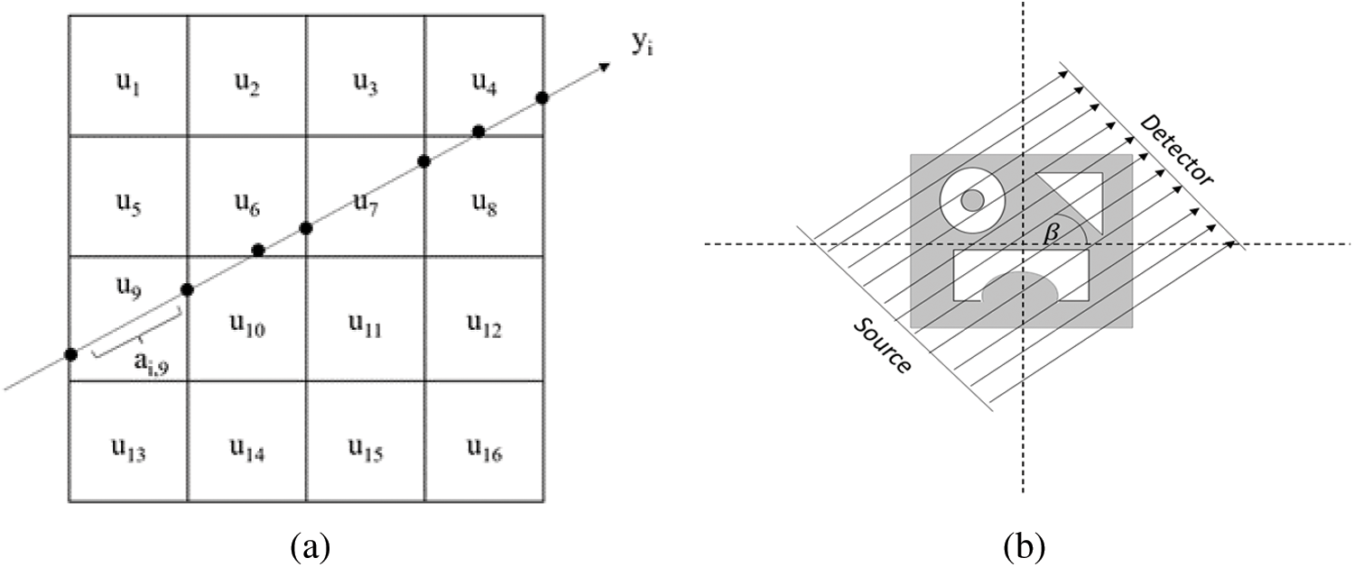
Figure 1: Mathematical model of discrete tomography. (a) Example of a projection value yi calculated from an image with 4 × 4 = 16 pixels, where yi is calculated by yi=ai,9u9+ai,10u10+ai,6u6+ai,7u7+ai,8u8+ai,4u4. (b) Geometry to measure a typical parallel-beam projection data with the rotation angle β around a coordinate origin

The image reconstruction problem is an inverse problem in which the image u is recovered from the projection data y using the matrix A, i.e.,

Find     u∈RN      s.t   y=Au.

In many cases of CT imaging, Eq. (1) is underdetermined because the number of measure projection data M  is substantially smaller than the number of unknowns N. Also, due to the noise in the projection data or errors in the projection model, the system of equations is inconsistent, such that the solution may be far from the truth. To address these issues, the reconstruction problem is typically expressed as a least-squares problem as

minu⁡ {f(u)≡12‖Au−y‖22}. (2)

For example, to solve this optimization problem, the following Newton-like algorithm can be used to find the image u [28].

uk+1=uk−λkHk−1∇f(uk),

where  λk  denotes the step-size parameter, Hk denotes an approximation of the Hessian matrix of f calculated at u=uk, and the gradient of f is given by

∇f(u)=AT(Au−y).

3  Basic Principle of Level-Set Method

In the areas of geometric inverse problems, such as shape optimization, image segmentation, and interface tracking, level-set methods have received a lot of attention due to their ability to adapt to topological changes in the region structures. In [29], Sethian and Osher introduced the classical level-set methods for solving the Hamiltonian-Jacobi equation, which is also known as a level-set equation.

∂ϕ∂t+F|∇ϕ|=0,

where ϕ:R2× R+→R denotes the level-set function and F denotes the normal velocity and this velocity is often calculated from the gradient of the cost function with respect to the parameters of the model [30,31].

3.1 Shape-Based Approach

In a large class of shape-based inverse problems [31–33], the model of interest u(x) is composed of two classes, namely foreground and background. Then, our objective is to determine the boundary between these classes and the characteristics that define the values of u in each class. Therefore, with any closed domain D⊆Ω with boundary δD, u(x) is modeled as

u(x)={uin            ∀ x∈Duex      ∀ x∈Ω∖D,

where uin denotes the value inside D and uex denotes the value outside D. Therefore, the corresponding model u(x) is represented as follows.

u(x)=uin(x) χD(x)+uex(x) (1−χD(x)),(3)

where χD(x) is the indicator function of D. From Eq. (3), u(x) cannot be differentiated on the boundary δD unlike what was stated earlier and finding the boundary in this case is the main objective. To solve this issue, the level-set function is known to be particularly useful. The level-set approach represents the region boundary by δD={x| ϕ(x)=0}  by using the zero contour of a higher-dimensional function ϕ(x). The function ϕ(x)  is called the level-set function [34,35], and the relation between ϕ(x) and D is expressed as

{ϕ(x)>0      ∀ x∈Dϕ(x)=0    ∀ x∈δD.ϕ(x)<0  ∀ x∈Ω∖D(4)

By using Eq. (4), the indicator function can be represented as χD(x)=H(ϕ(x)), where H is the Heaviside function defined by H(⋅)=12(1+sign(⋅)). As a result, u(x) can be represented by

u(x)=uin(x) H(ϕ(x))+uex(x) (1−H(ϕ(x))). (5)

3.2 Parametric Level-Set

In many existing shape-based approaches, the level-set function ϕ(x) is selected as a signed distance function [36]. As an alternative to this classical approach of level-set functions, consider that the level-set function is not only a function of x but also a function of parameters α=[α1,  α2, ….., αN]∈RN. Based on this parameterization, the level-set function can be defined as a parametric level-set (PALS), and we can modify Eq. (4) as follows

{ϕ(x,α)>c      ∀ x∈Dϕ(x,α)=c    ∀ x∈δD,ϕ(x,α)<c   ∀ x∈Ω∖D    (6)

where c is a positive small value. Now, we can say that for some specified α, ϕ(x,α) can explicitly determine the level-set function for the entire domain Ω. By updating α, the required evolution of ϕ is performed to solve the underlying inverse problems. Based on Eq. (6), the model u(x) in Eq. (5) is expressed as

u(x,α)=uin(x) H(ϕ(x,α)−c)+uex(x) (1−H(ϕ(x,α)−c)). (7)

A PALS function is an example of a basis expansion using known basis functions and unknown weights. As a result of this statement, the level-set function ϕ(x) may be represented parametrically by using the set of RBFs  Bi(x)(i=1,2,⋯,N) as follows [37].

ϕ(x,α)=∑i=1N⁡αiBi(x), (8)

where N denotes the number of RBFs, and α=[α1,  α2, ….., αN]∈RN are unknown parameters of ϕ(x,α) that determine the weight attached to each Bi(x). The meaning of Eq. (8) is that ϕ(x,α) is represented by a linear combination of basis functions  Bi(x)(i=1,2,⋯,N) taken with the weights α. There are several basis set choices available, including Gaussian, multi-quadric, poly-harmonic splines, and thin spline polynomial. Here, the Gaussian radial-basis function (GRBF) is used, and it is expressed as

Bi(x)=exp(−‖x−xi‖22σ2),  (9)

where σ is the width of Gaussian, xi is the center of GRBF, and ‖⋅‖ is the Euclidean norm.

4  Shape Representation and Algorithms

In this section, we describe the method for reconstructing the image using the parametric level-set and how it evolves when parameters α and GRBFs are updated. Consider the level-set represented in Fig. 2. In Fig. 2, we illustrate how a smooth shape discretized on a grid of N=125×125 can be reconstructed.

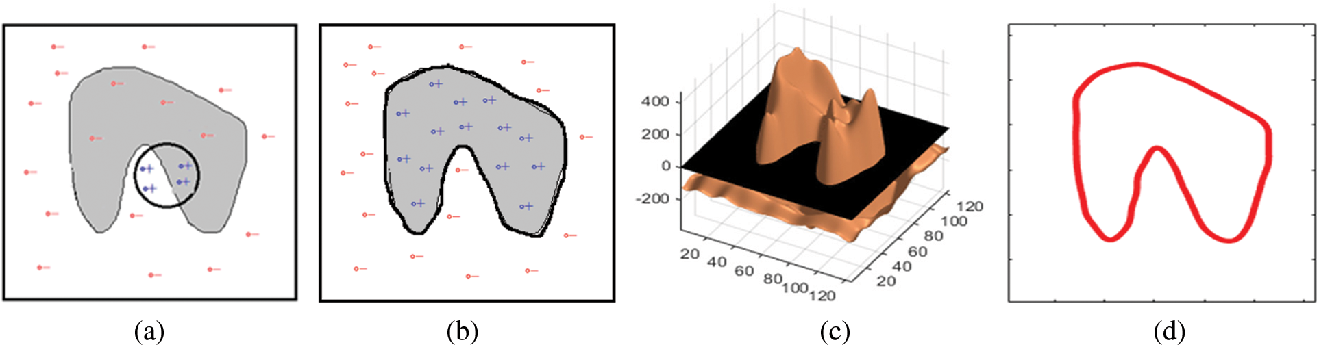
Figure 2: This figure shows an example of reconstruction using the parametric level-set functions by GRBFs. (a) The black contour is the resulting c-level set of the initial PALS function, and it is defined by a boundary between the region having positive, i.e., ϕ(x,α)>c, values of GRBFs denoted by ‘+’ (blue) sign, and the region having negative, i.e., ϕ(x,α)<c, values of GRBFs denoted by ‘-’ (red) sign. (b) shows the reconstructed shape by using the parametric level-set. (c) and (d) show the final level-set function ϕ(x,α)  and the corresponding boundary of the shape δD

Next, we discuss how to select the Gaussian width parameter σ of GRBF in the PALS reconstruction. For this purpose, we rewrite the GRBF basis function of Eq. (9) in the alternative form as

Bi(x)=exp(−β∥x−xi∥)2,

where β=(2 σ)−1. Obviously, by changing the parameter value β, i.e., the width σ of GRBF, representation power of the method will be changed significantly. The spreading parameter β is very important. In particular, β has a large effect on the recovery accuracy (representation power) when the number of GRBFs placed in the 2-D plane is small. In our experiments, we discretized our model on a cartesian grid with 125×125  pixels, and the nodes to place the GRBFs were selected as a sparse cartesian grid with 28×28 pixels, i.e., N = 784. The PALS reconstruction process was initialized with a very rough representation with N = 10 GRBFs and β=0.1. As shown in Fig. 2, this model is finally discretized on a Cartesian grid. Therefore, by using Eq. (7) in Eq. (2), the discretized reconstruction problem for the parametric level-set method can be expressed as

minα⁡ {f(α)≡12‖A[uin H(ϕ(x,α)−c)+uex (1−H(ϕ(x,α)−c))]−y‖22}. (10)

To calculate the gradient of Eq. (10), taking the derivative of Eq. (7) with respect to ϕ gives

 ∂u∂ϕ=(uin−uex )δ(ϕ−c),(11)

where δ(ϕ−c) is Dirac delta function [38,39]. Using the chain rule, we have

∂u∂α=∂u∂ϕ∂ϕ∂α=BT(uin−uex )δ(ϕ−c),  (12)

In Eq. (12), B is the matrix constructed by the basis vectors of GRBF, i.e., matrix converting the parameters α into the level-set function ϕ(x,α). Using Eq. (12), the gradient of cost function f is obtained as follows.

∇f(α)=∂f∂u∂u∂α=BT(uin−uex )δ(ϕ−c)ATR(α), (13)

where the residual operator R(α) is defined by

R(α)=A[uin H(ϕ(x,α)−c)+uex (1−H(ϕ(x,α)−c))]−y.  (14)

In our implementation, we solve the minimization problem of Eq. (10) with respect to the level-set parameters α by using the quasi-Newton method with the L-BFGS method to approximate the Hessian Hk−1 [40]. The iteration formula is expressed as

αk+1=αk−λkHk−1∇f(αk).

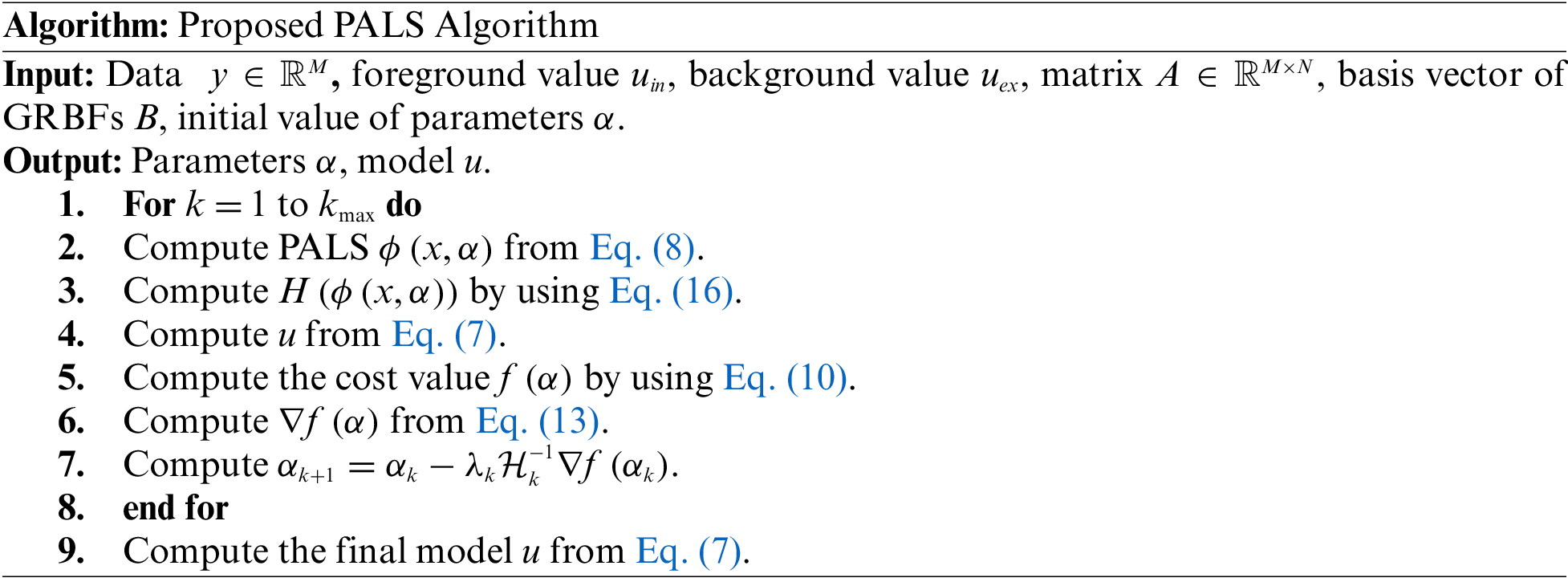
The final reconstruction algorithm is summarized in Algorithm below.

From Eq. (5), during the optimization process, we need to compute Heaviside function H(⋅) from the level-set function ϕ(x,α). As a smooth approximation of the Heaviside function, we can use the following C∞ regularization of H(⋅) [34].

H(x)=12(1+2πarctan(πxϵ)). (15)

However, Eq. (15) is not a good choice due to the following reason. Considering the nature of parametric level-set function, Eq. (7) shows that H(ϕ(x,α))=1 for every x∈D and H(ϕ(x,α))=0 for any x∈Ω∖D. According to Fig. 3, using the C∞ regularization of the Heaviside function means that the resulting parametric level-set function by using GRBFs takes a relatively large positive value in the region D and a rather large negative value outside the region D. To avoid this problem, we use the following C2 regularization of Heaviside function [38].

H(x)={1                                       x>ϵ0                                      x<−ϵ12+x2ϵ+12πsin⁡(πxϵ)      |x|  ≤ϵ.(16)

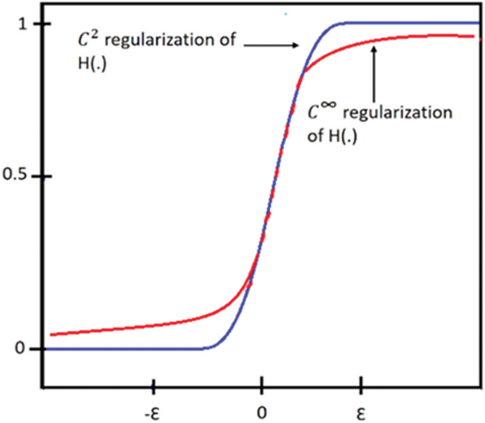
Figure 3: Comparison of two regularized versions of Heaviside function H(⋅)

A final remark on solving the under-determined inverse problems is as follows. Our original cost function to solve the under-determined CT reconstruction is the standard least-squares error of Eq. (2). In the setup of sparse-view CT and limited-angle CT, however, due to the lack of sufficient projection data, we normally need to include a regularization term into the cost function. In the proposed method, instead of using the regularization term, we have used the deterministic constraint that the image can be expressed by the simple model of Eq. (7). Since the dimension to represent the image in this model is essentially very small, it works similarly to the regularization. In this model-based approach, the detailed form of the cost function for image reconstruction cannot be explicitly written, unlike the case of using the regularization term.

5  Numerical Experiments

In this section, we describe experimental results for image reconstruction in sparse-view CT and limited-angle CT. The experiments were performed by using synthetic images and real X-ray CT projection data of a carved cheese slice [41]. We compared the proposed method to some of the state-of-the-art reconstruction methods for binary tomography. In Section 5.1, we will discuss the details of the compared methods.

For the experiments with synthetic images, we used four images shown in Fig. 4. All these binary images consist of 125×125  pixels. We considered standard parallel-beam geometry, in which every detector consists of 125 pixels. For the case of sparse-view CT, the number of projection data uniformly sampled over the angular range [0,π) was set to 10, 8, 6, and 4.  Our aim is to decrease scanning time in sparse-view CT by reducing the number of angles. For the case of limited-angles CT, we considered four different angular coverages π/2, 7π/12, 2π/3, and 5π/6. Finally, we evaluated the performance of the proposed method by adding different levels of Gaussian noise to the projection data, where the noise level was 0.1%, 5%, and 10%. Up to the 5% noise case, the proposed method could stably reconstruct a reasonable image.

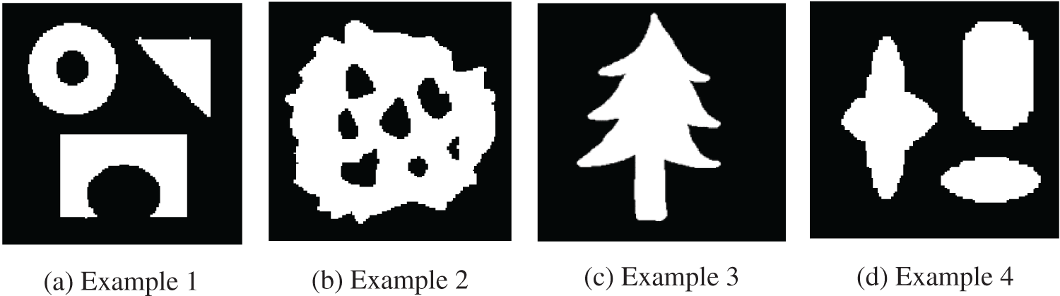
Figure 4: These four synthetic images were used to evaluate the performance of the proposed approach

5.1 Other Reconstruction Methods Used for Comparison

There are several reconstruction methods for tomography. We are focusing on the following four methods, which have been developed for binary tomography aiming at reconstructing nice images with limited projection data.

First: Total-variation (TV) method based on solving the following optimization problem.

minx⁡ ‖Ax−y‖2+λ‖Dx‖1, 

λ denotes the regularization parameter, and D is the matrix that captures the horizontal and vertical discrete gradients. The above problem was solved using the Chambolle-Pock method in [42].

Second: Dual Problem (DP) method proposed by Kadu and Van Leeuwen [43], which is based on solving the following so-called Largrangian dual problem.

x∗=argminx⁡ 12‖x−y‖2+‖ATx‖1,   

where x∗  denotes an optimal dual variable. This method is a convex formulation based on Lagrangian dual of the binary constrained least-squares problem, and they solved this problem by using L-BFGS Quasi-Newton method [43,44].

Third: Batenburg and Sijbers proposed the Discrete Algebraic Reconstruction Technique (DART) in [16]. Although DART works well for a large class of binary images by exploiting the prior knowledge on gray levels in each region of the image, our proposed method is still better and can compare favorably with this method.

Fourth: The parametric level-set (PALS) representation proposed by Kadu et al. [27]. In their work, they used C4-smooth Wendland’s function (1−r)+8(32r3+25r2+8r+1) as the radial-basis function (RBF), and the corresponding PALS function is expressed as

ϕ(x)=∑i=1L⁡αiψ(β‖x−ξi‖2),  

where ψ(⋅)  denotes each RBF, L denotes the number of RBFs, ξi is the center to place RBF, and β is a scaling parameter.

5.2 Sparse-View CT Case

In Fig. 5, we show reconstructed images for Example 1 when the number of projection data is 4. From the results, the proposed method provided an image that is very close to the ground truth compared to the other methods.

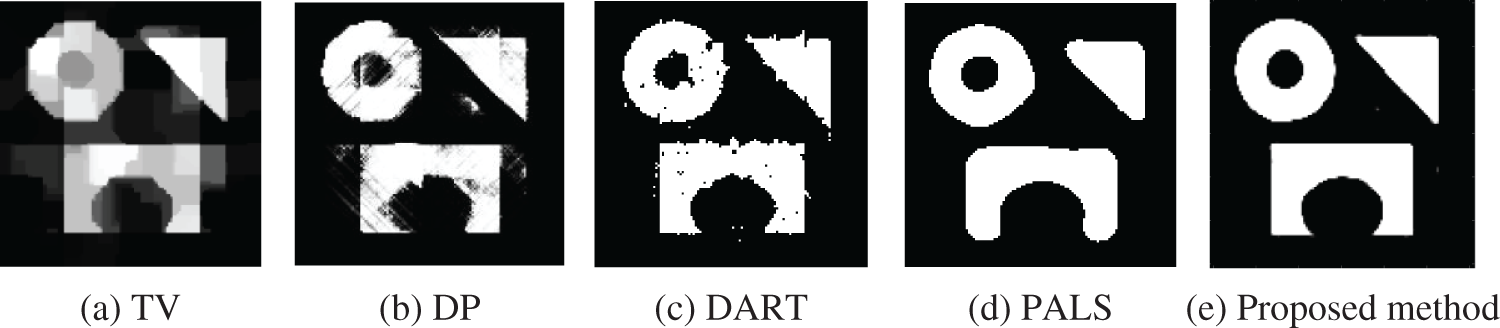
Figure 5: Reconstructed images from only 4 projection data uniformly distributed over the angular range [0,π) for Example 1

Fig. 6 shows the performance of our proposed method when the number of projection data is changed between 4 and 10. We find that our method can reconstruct a reasonable image with as few as 5 projection data.

Figure 6: Reconstructed images for Example 2. The number of projection data was changed between 4 and  10

In addition to the synthetic images, we applied the proposed method to real X-ray CT projection data of a carved cheese slice [41]. In Fig. 7, we show the measured sinogram and the corresponding Filtered Back Projection (FBP) reconstruction from 180 projection data measured over the angular range [0,2π). The object can be observed to be approximately binary, consisting of only two gray levels, representing cheese region and air region. Now, we will show the performance of the proposed method with this data. Fig. 8 shows the comparison between the proposed method and the other methods. In Fig. 9, we show object boundaries (red contours) reconstructed from 45, 23, 12, and 8 projection data. We observe that the proposed method provided nice images with a small number of projection data.

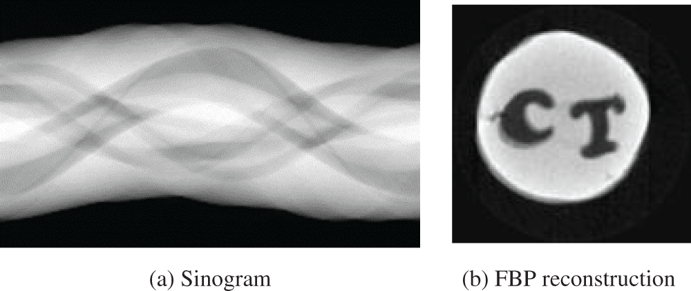
Figure 7: Sinogram and a reconstructed image of the carved cheese real data. The number of projection data was 180 over the angular range [0,2π)

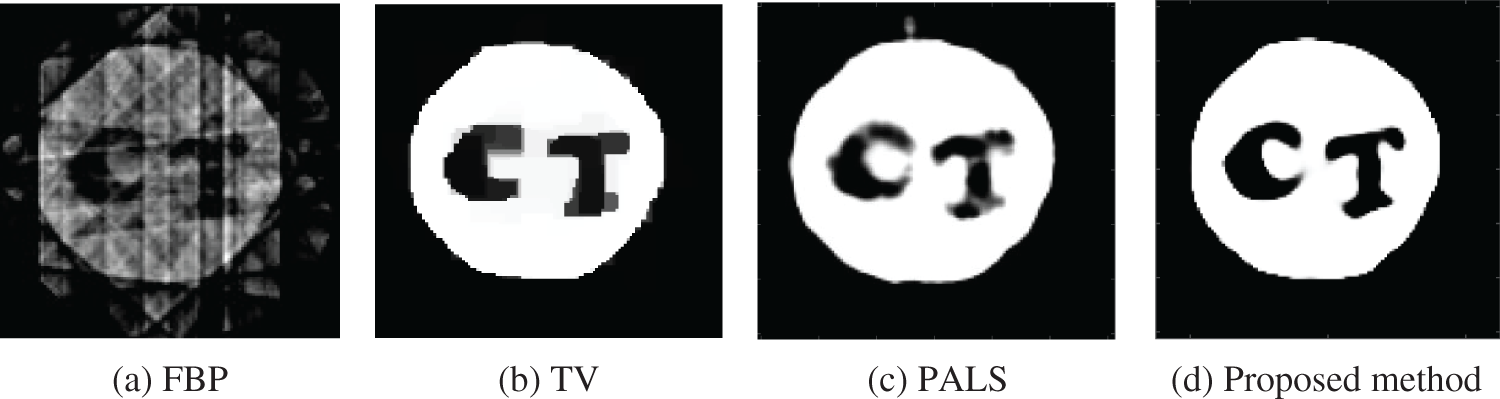
Figure 8: Reconstructed images for the carved cheese real data from only 8 projection data uniformly distributed over the angular range [0,π)

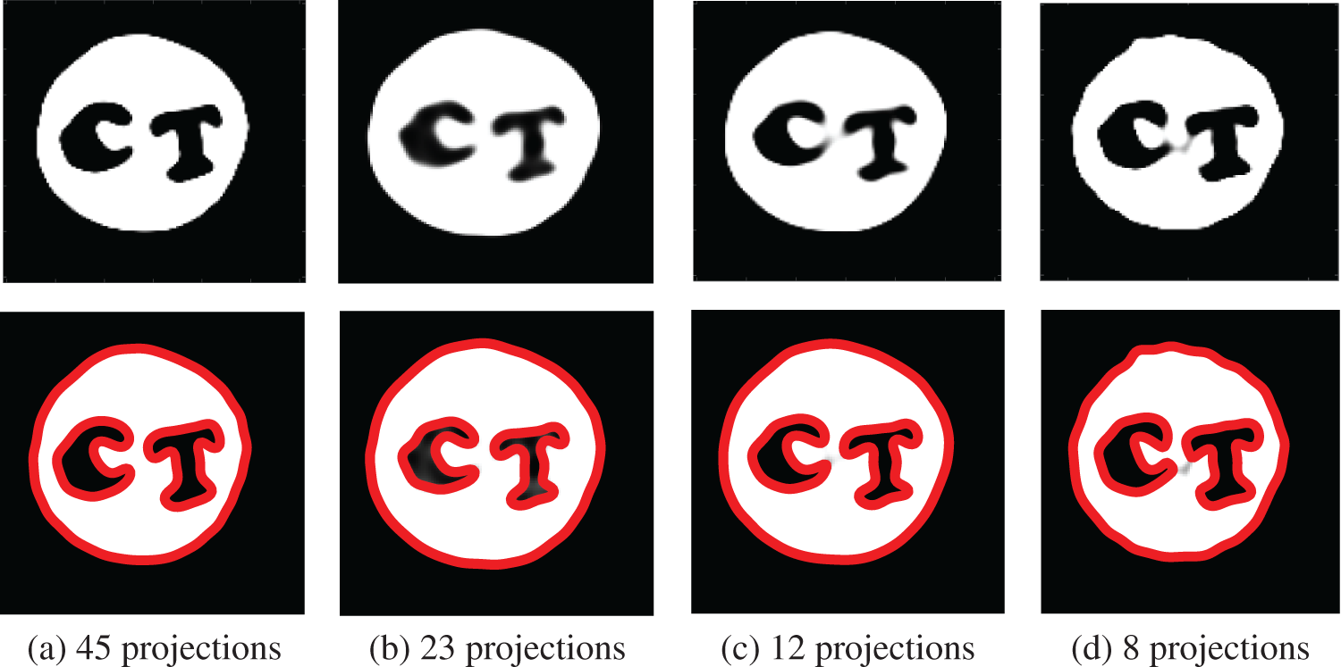
Figure 9: Reconstructed images from sparse-view projection data by the proposed method for the carved cheese real data. The red contours represent the reconstructed boundary of object

5.3 Limited-Angle CT Case

In the case of limited-angle CT, the problem becomes much more difficult, but the proposed method still works well, and the reconstructed images were very close to the true images. For example, Fig. 10 shows the images by the proposed method and the other reconstruction methods for Example 3. In this experiment, the number of projection data was only 5 and the angular range was set to [0,π/2).

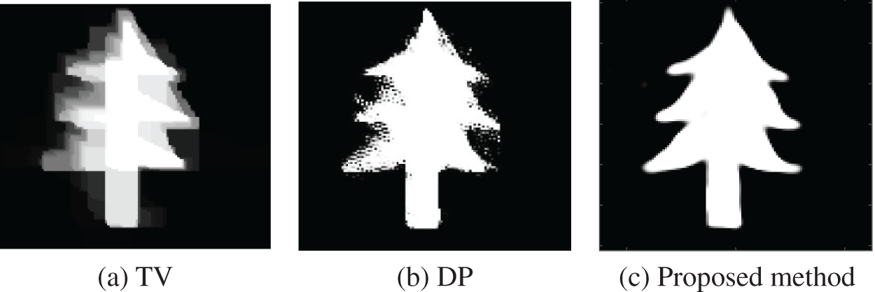
Figure 10: Reconstructed images from only 5 projection data uniformly distributed over the angular range [0,π/2)

In Fig. 11, we show how reconstructions by the proposed method vary by decreasing the angular range for Example 4. In CT fields, it is well-known for a long time that it is difficult to reconstruct images with sufficient accuracy from limited-angle projection data. However, as shown in Fig. 11, we could reconstruct almost correct images even when the angular range was [0,π/2). This is clearly thanks to the use of binary constraint.

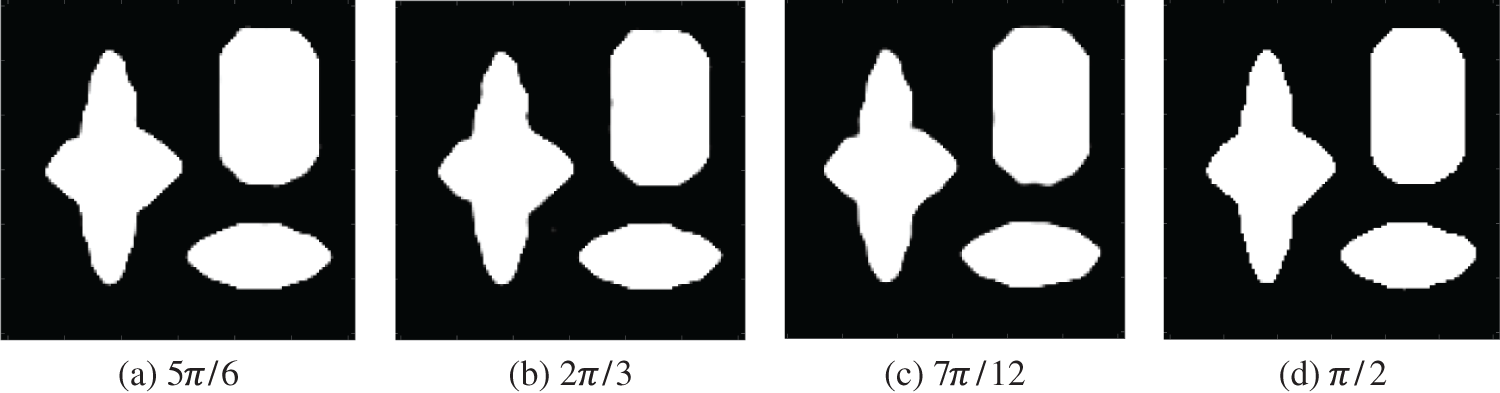
Figure 11: Reconstructed images for Example 4 in the limited-angle CT case. The number of projection data was 4 and the angular range to measure the projection data was set to 5π/6, 2π/3, 7π/12, and π/2

For the real data, in Figs.12 and 13, we show reconstructed images by the proposed method when the angular range was limited to [0,π/2), where the number of projection data was set  to 14, 10, and 8. We observe that it is still possible to correctly identify the existence of letters C and T.

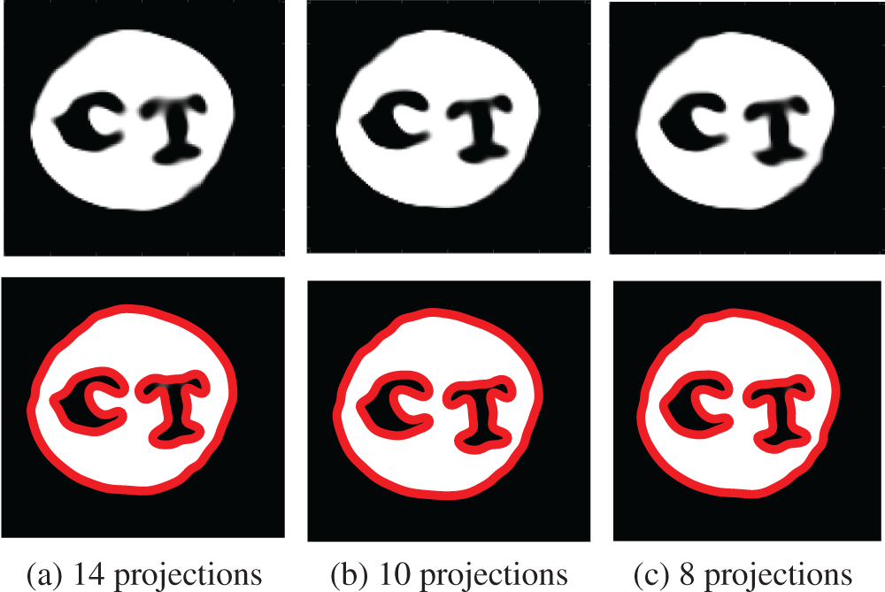
Figure 12: Reconstructed images for the carved cheese real data in the limited-angle case. The angular range to measure the projection data was set to [0,π/2)

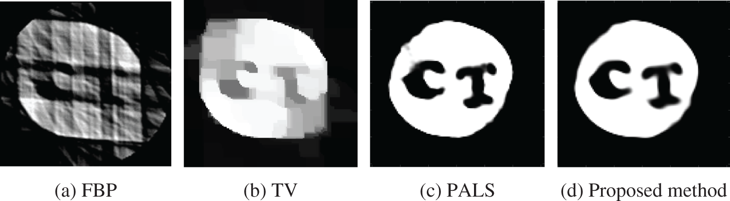
Figure 13: Reconstructed image for the real data from only 8 projection data for real data in the limited-angle case, where the angular range was limited to [0,π/2)

5.4 Evaluation of Effect of Noise

We evaluated the performance of the proposed method in the presence of three different levels of noise in the projection data. We added Gaussian noise with ratio 0.1%, 5%, and 10% to the projection data, from which image reconstruction was performed. In Fig. 14, we show reconstructed images for Example 1 and Example 2. We observe that the proposed method is stable in the presence of modest amounts of noise but degrades gradually as the noise level increases.

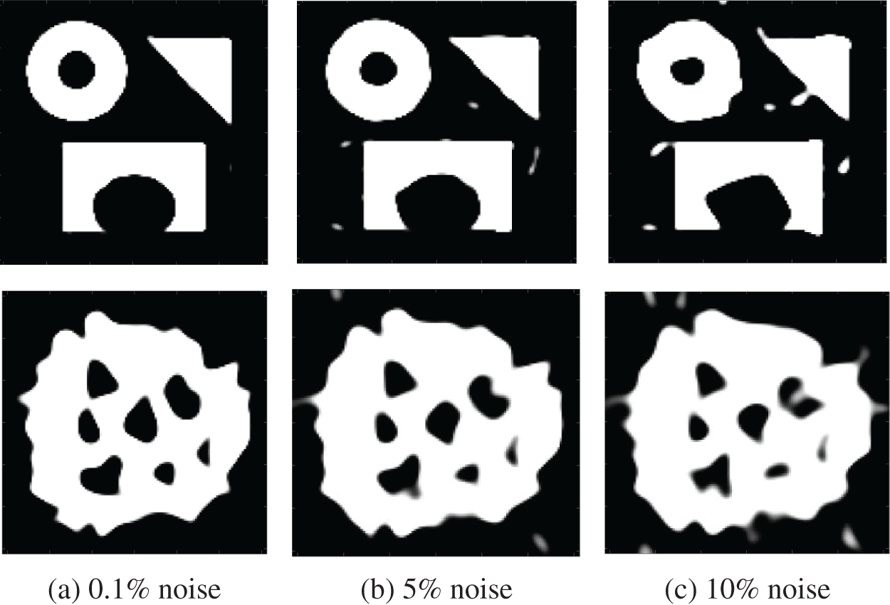
Figure 14: Reconstructed images for Example 1 and Example 2 when the projection data contains noise, where the ratio of noise was set to 0.1%, 5%, and 10%

6  Conclusions

In this paper, we proposed a novel approach using a parametric level-set method for image reconstruction in binary tomography. The basic formulation of the problem is summarized as follows. Shapes of objects are represented via a level-set function, which is represented by using a Gaussian radial basis function (GRBF). We are using an appropriate parametrization of the level-set function, which can reduce the problem dimension and essentially regularizes the problem in a successful way. Based on this modeling, the level-set function is more likely to behave well, so it doesn’t need re-initialization like the traditional methods. Furthermore, unlike the use of traditional level-set methods, the problem to be solved for image reconstruction becomes a tractable convex optimization. We solved the optimization problem using a Newton-type method because the number of underlying parameters in a parametric level-set approach is usually much smaller than the number of pixels that we finally would like to get the image by discretizing the level-set function. We tested the proposed method on synthetic images and real data. According to our experiments, the proposed approach compares favorably with some state-of-the-art reconstruction methods, and it is also relatively stable in the presence of modest amount of noise.

Acknowledgement: Real projection data used in this study is available from the members of the X-ray lab at the Faculty of Science, University of Helsinki, Finland upon request http://www.fips.fi/dataset.php. We greatly appreciate them to provide us with the data. We also thank four anonymous reviewers for their comments, which significantly improved the manuscript.

Funding Statement: This work was supported by JST-CREST Grant Number JPMJCR1765, Japan.

Conflicts of Interest: The authors declare that they have no conflicts of interest to report regarding the present study.

References

 1.  A. C. Kak and M. Slaney, “Principles of computerized tomographic imaging,” Society for Industrial and Applied Mathematics, 2001. [Google Scholar]

 2.  S. R. Deans, “The Radon transform and some of its applications,” in A Wiley-Interscience Publication, New York, 2007. [Google Scholar]

 3.  X. R. Zhang, X. Sun, W. Sun, T. Xu and P. P. Wang, “Deformation expression of soft tissue based on BP neural network,” Intelligent Automation & Soft Computing, vol. 32, no. 2, pp. 1041–1053, 2022. [Google Scholar]

 4.  W. Chen, T. Sun, F. Bi, T. Sun, C. Tang et al., “Overview of digital image restoration,” Journal of New Media, vol. 1, no. 1, pp. 35–44, 2019. [Google Scholar]

 5.  A. Dermanis, A. Grun and F. Sanso, “Geomatics methods for the analysis of data in the earth sciences,” in Springer, Berlin, Heidelberg, Germany, 2000. [Google Scholar]

 6.  J. Kastner, “Conference on industrial computed tomography (ICT),” in Proc., Shaker Verlag, Aachen, Germany, 2012. [Google Scholar]

 7.  T. M. Buzug, “Computed tomography,” Springer handbook of medical technology, Springer, Berlin, Heidelberg, 2011. [Google Scholar]

 8.  G. T. Herman and A. Kuba, “Discrete tomography: Foundations, algorithms, and applications,” in Springer, Boston, 1999. [Google Scholar]

 9.  P. A. Midgley and R. E. Dunin-Borkowski, “Electron tomography and holography in materials science,” Nature Materials, vol. 8, no. 4, pp. 271–280, 2009. [Google Scholar]

10. M. T. Buzug, “Computed tomography: From photon statistics to modern cone-beam CT,” in Springer, 2008. [Google Scholar]

11. J. Gregor and T. Benson, “Computational analysis and improvement of SIRT,” IEEE Transactions on Medical Imaging, vol. 27, no. 7, pp. 918–924, 2008. [Google Scholar]

12. E. Y. Sidky, M. C. Kao and X. Pan, “Accurate image reconstruction from few-views and limited-angle data in divergent-beam CT,” Journal of X-ray Science and Technology, vol. 14, no. 2, pp. 119–139, 2006. [Google Scholar]

13. X. Tai and J. Duan, “A simple fast algorithm for minimization of the elastica energy combining binary and level set representations,” International Journal of Numerical Analysis and Modeling, vol. 14, no. 6, pp. 809–821, 2017. [Google Scholar]

14. L. Gorelick, O. Veksler, Y. Boykov and C. Nieuwenhuis, “Convexity shape prior for binary segmentation,” IEEE Transactions on Pattern Analysis and Machine Intelligence, vol. 39, no. 2, pp. 258–271, 2017. [Google Scholar]

15. S. Yan, X. Tai, J. Liu and H. Huang, “Convexity shape prior for level set-based image segmentation method,” arXiv preprint arXiv:1805.08676, 2018. [Google Scholar]

16. K. J. Batenburg and J. Sijbers, “DART: A practical reconstruction algorithm for discrete tomography,” IEEE Transactions on Image Processing, vol. 20, no. 9, pp. 2542–2553, 2011. [Google Scholar]

17. F. J. Maestre-Deusto, G. Scavello, J. Pizarro and P. L. Galindo, “ADART: An adaptive algebraic reconstruction algorithm for discrete tomography,” IEEE Transactions on Image Processing, vol. 20, no. 8, pp. 2146–2152, 2011. [Google Scholar]

18. N. Antal, “Smoothing filters in the DART algorithm. Combinatorial image analysis,” Springer, Lecture Notes in Computer Science, vol. 8466, pp. 224–237, 2014. [Google Scholar]

19. K. J. Batenburg, “3D imaging of nanomaterials by discrete tomography,” Ultramicroscopy, vol. 109, no. 6, pp. 730–740, 2009. [Google Scholar]

20. A. Zürner, M. Döblinger, V. Cauda, R. Wei and T. Bein, “Discrete tomography of demanding samples based on a modified SIRT algorithm,” Ultramicroscopy, vol. 115, pp. 41–49, 2012. [Google Scholar]

21. K. J. Batenburg and J. Sijbers, “Discrete tomography from micro-CT data: Application to the mouse trabecular bone structure,” Medical Imaging 2006: Physics of Medical Imaging, vol. 6142, pp. 1325–1335, 2006. [Google Scholar]

22. W. Van Aarle, K. J. Batenburg, G. Van Gompel, E. Van de Casteele and J. Sijbers, “Super-resolution for computed tomography based on discrete tomography,” IEEE Transactions on Image Processing, vol. 23, no. 3, pp. 1181–1193, 2014. [Google Scholar]

23. H. Segers, W. J. Palenstijn, K. J. Batenburg and J. Sijbers, “Discrete tomography in MRI: A simulation study,” Fundamenta Informaticae, vol. 125, pp. 223–237, 2013. [Google Scholar]

24. M. Kilmer, E. Miller, M. Enriquez and D. Boas, “Cortical constraint method for diffuse optical brain imaging,” Advanced Signal Processing Algorithms Architectures, and Implementations, vol. 5559, pp. 381–391, 2004. [Google Scholar]

25. A. Gelas, O. Bernard, D. Friboulet and R. Prost, “Compactly supported radial basis functions-based collocation method for level-set evolution in image segmentation,” IEEE Transactions on Image Processing, vol. 16, no. 7, pp. 1873–1887, 2007. [Google Scholar]

26. O. Bernard, D. Friboulet, P. Thévenaz and M. Unser, “Variational B-spline level-set: A linear filtering approach for fast deformable model evolution,” IEEE Transactions on Image Processing, vol. 18, no. 6, pp. 1179–1191, 2009. [Google Scholar]

27. A. Kadu, T. van Leeuwen and W. A. Mulder, “Salt reconstruction in full-waveform inversion with a parametric level-set method,” IEEE Transactions on Computational Imaging, vol. 3, no. 2, pp. 305–315, 2017. [Google Scholar]

28. R. G. Pratt, C. Shin and J. G. Hick, “Gauss-newton and full newton methods in frequency–Space seismic waveform inversion,” Geophysical Journal International, vol. 133, no. 2, pp. 341–362, 1998. [Google Scholar]

29. S. Osher and J. A. Sethian, “Fronts propagating with curvature-dependent speed: Algorithms based on hamilton-jacobi formulations,” Journal of Computational Physics, vol. 79, no. 1, pp. 12–49, 1988. [Google Scholar]

30. M. Burger, A level set method for inverse problems,” Inverse Problems, vol. 17, no. 5, pp. 1327, 2001. [Google Scholar]

31. O. Dorn and D. Lesselier, “Level set methods for inverse scattering,” Inverse Problems, vol. 22, no. 4, pp. R67–R131, 2006. [Google Scholar]

32. F. Santosa, “A Level-set approach for inverse problems involving obstacles fadil santosa,” ESAIM: Control, Optimization and Calculus of Variations, vol. 1, pp. 17–33, 1996. [Google Scholar]

33. A. Aghasi and J. Romberg, “Sparse shape reconstruction,” SIAM Journal on Imaging Sciences, vol. 6, no. 4, pp. 2075–2108, 2013. [Google Scholar]

34. A. Aghasi, M. Kilmer and E. L. Miller, “Parametric level set methods for inverse problems,” SIAM Journal on Imaging Sciences, vol. 4, pp. 618–650, 2011. [Google Scholar]

35. S. Osher and R. P. Fedkiw, “Level set methods: An overview and some recent results,” Journal of Computational Physics, vol. 169, no. 2, pp. 463–502, 2001. [Google Scholar]

36. M. Soleimani, W. Lionheart and O. Dorn, “Level set reconstruction of conductivity and permittivity from boundary electrical measurements using experimental data,” Inverse Problems in Science and Engineering, vol. 14, no. 2, pp. 193–210, 2006. [Google Scholar]

37. H. A. Ali and H. Kudo, “New level-set-based shape recovery method and its application to sparse-view shape tomography,” in 2021 4th Int. Conf. on Digital Medicine and Image Processing, Kyoto, Japan, pp. 24–29, 2021. [Google Scholar]

38. H. K. Zhao, T. Chan, B. Merriman and S. Osher, “A variational level set approach to multiphase motion,” Journal of Computational Physics, vol. 127, no. 1, pp. 179–195, 1996. [Google Scholar]

39. H. Y. Tian, S. Reutskiy and C. S. Chen, “A basis function for approximation and the solutions of partial differential equations,” Numerical Methods for Partial Differential Equations: An International Journal, vol. 24, no. 3, pp. 1018–1036, 2008. [Google Scholar]

40. M. W. Schmidt, E. Berg, M. Friedlander and K. Murphy, “Optimizing costly functions with simple constraints: A limited-memory projected quasi-newton algorithm,” in International Conference on Artificial Intelligence and Statistics, Florida, USA, vol. 5, pp. 456–463, 2009. [Google Scholar]

41. T. A. Bubba, M. Juvonen, J. Lehtonen, M. März, A. Meaney et al., “Tomographic X-ray data of carved cheese,” arXiv preprint arXiv:1705.05732, 2017. [Google Scholar]

42. A. Chambolle and T. Pock, “A First-order primal-dual algorithm for convex problems with applications to imaging,” Journal of Mathematical Imaging and Vision, vol. 40, no. 1, pp. 120–145, 2011. [Google Scholar]

43. A. Kadu and T. van Leeuwen, “A convex formulation for binary tomography,” IEEE Transactions on Computational Imaging, vol. 6, pp. 1–11, 2019. [Google Scholar]

44. D. C. Liu and J. Nocedal, “On the limited memory bfgs method for large scale optimization,” Mathematical Programming, vol. 45, no. 1–3, pp. 503–528, 1989. [Google Scholar]

This work is licensed under a Creative Commons Attribution 4.0 International License, which permits unrestricted use, distribution, and reproduction in any medium, provided the original work is properly cited.