Computers, Materials & Continua DOI:10.32604/cmc.2022.030428
Article

Optimal Deep Canonically Correlated Autoencoder-Enabled Prediction Model for Customer Churn Prediction

Olfat M. Mirza1, G. Jose Moses2, R. Rajender3, E. Laxmi Lydia4, Seifedine Kadry5, Cheadchai Me-Ead6 and Orawit Thinnukool7,*

1Department of Computer Science, College of Computers and Information Systems, Umm Al-Qura University, Makkah, Saudi Arabia
2Department of Computer Science Engineering, Malla Reddy Engineering College, 500100, India
3Department of Computer Science Engineering, Lendi Institute of Engineering & Technology, Denkada, 535005, India
4Department of Computer Science and Engineering, Vignan’s Institute of Information Technology, Visakhapatnam, 530049, India
5Department of Applied Data Science, Noroff University College, Norway
6Program in Statistics and Information Management, Faculty of Science, Maejo University, Chiang Mai, 50290, Thailand
7Department of Modern Management and Information Technology, College of Arts Media and Technology, Chiang Mai University, Chiang Mai, 50200, Thailand
*Corresponding Author: Orawit Thinnukool. Email: orawit.t@cmu.ac.th
Received: 25 March 2022; Accepted: 07 May 2022

Abstract: Presently, customer retention is essential for reducing customer churn in telecommunication industry. Customer churn prediction (CCP) is important to predict the possibility of customer retention in the quality of services. Since risks of customer churn also get essential, the rise of machine learning (ML) models can be employed to investigate the characteristics of customer behavior. Besides, deep learning (DL) models help in prediction of the customer behavior based characteristic data. Since the DL models necessitate hyperparameter modelling and effort, the process is difficult for research communities and business people. In this view, this study designs an optimal deep canonically correlated autoencoder based prediction (O-DCCAEP) model for competitive customer dependent application sector. In addition, the O-DCCAEP method purposes for determining the churning nature of the customers. The O-DCCAEP technique encompasses pre-processing, classification, and hyperparameter optimization. Additionally, the DCCAE model is employed to classify the churners or non-churner. Furthermore, the hyperparameter optimization of the DCCAE technique occurs utilizing the deer hunting optimization algorithm (DHOA). The experimental evaluation of the O-DCCAEP technique is carried out against an own dataset and the outcomes highlighted the betterment of the presented O-DCCAEP approach on existing approaches.

Keywords: Churn prediction; customer retention; deep learning; machine learning; archimedes optimization algorithm

1  Introduction

Customer retention plays a significant part in predicting churn, and telecommunication system is straightaway connected to the financial corporations. Henceforth, several businesses executed dissimilar activities for emerging a strong connection with user and to decrease user defection. Recently, the cost cutting stress and competing nature raised the companies to exploit the customer relationship management (CRM) system [1]. Customer Churn prediction (CCP) is assisted to established approaches for customer retention. In consort with rising competitiveness in market for offering facilities, the hazard of customer churn exponentially rises [2]. Then, establishing approaches to follow loyal customers (non-churner) becomes an obligation. The customer churn model aims at identifying earlier [3,4] churn signals and attempting to forecast the customer that leaves willingly. Therefore, several firms have understood that the current dataset is one of the valued advantages [5], and based on Abbasdimehr, churn prediction is a valuable mechanism for predicting customers at risk. For capturing the abovementioned issue, corporation must forecast the customer behavior properly. Customer churn management is performed by: (1) Reactive and (2) Proactive manners. In the reactive method, corporations wait for the termination request established from the user, then, business provides the effective strategies to the user for retention [6,7]. It is a binary classifier issue in which churner is detached from the non-churner. For resolving the challenge, machine learning method has shown an effectual method, for predicting data according to formerly taken information [8,9]. In machine learning (ML) model, afterward, pre-processing feature selection performs a substantial part to enhance the classifier performance. Several techniques are proposed by authors for feature selection that is effective for reducing the overfitting, dimension, and computational difficulty [10].

Pustokhina et al. [11] proposed a dynamic CCP approach to business intelligence utilizing text analytics with metaheuristic optimization (CCPBI-TAMO) technique. Also, the chaotic pigeon inspired optimization based feature selection (CPIO-FS) approach was utilized to FS procedure and decreased computation complexity. Also, the long short term memory (LSTM) with stacked autoencoder (SAE) technique was executed for classifying the feature decreased data. Lastly, the sunflower optimization (SFO) hyper-parameter tuning procedure occurs to enhance the CCP performance. In [12], a new algorithmic extension, spline-rule ensembles (SRE) with sparse group lasso regularization (SRE-SGL) was presented for enhancing interpretability with infrastructure regularized. The experiments on 14 real world customer churn datasets from distinct industries illustrate the higher prediction performance of SRE.

Bilal et al. [13] presented a hybrid method that is dependent upon integration of clustering and classification techniques utilizing an ensemble. Primary, distinct clustering techniques (for instance K-medoids, random clustering, K-means, and X-means) are calculated separately on 2 churn prediction data sets. Next, the hybrid methods are established by integrating the cluster with 7 various classifier approaches separately afterward evaluation was executed utilizing ensembles.

Wu et al. [14] presented an enhanced forecast method by combining data pre-processed and ensemble learning for solving these 2 problems. In specially, 2 novel features were initially combined for optimum capturing customer behavior. Second, the principal component analysis (PCA) was implemented for reducing data dimensions. Tertiary, adaptive boosting (AdaBoost) was utilized for cascading several DL for minimizing the influences in the unbalanced data. Ramesh et al. [15] examine the effectual solution for all these challenging problem from CCP. The analysis utilizes data sets from the telecommunication industry, the artificial neural network (ANNs) and random forest (RF) for determining the features that stimulate consumer churn. A hybrid ANN based work was presented to forecast CCP.

This study designs an optimal deep canonically correlated autoencoder based prediction (O-DCCAEP) model for competitive customer dependent application sector. In addition, the O-DCCAEP approach purposes for determining the sentiment of the customers. The O-DCCAEP technique encompasses pre-processing, classification, and hyperparameter optimization. Furthermore, the DCCAE model is employed to classify the churners or non-churner. Furthermore, the hyperparameter optimization of the DCCAE technique occurs using the deer hunting optimization algorithm (DHOA). The experimental evaluation of the O-DCCAEP technique is carried out against an own dataset and the outcomes highlighting the betterment of the presented O-DCCAEP approach on the existing approaches.

The rest of the paper is organized as follows. Section 2 offers the proposed model and Section 3 discusses performance validation. Lastly, Section 4 concludes the paper.

2  Process Involved in O-DCCAEP Model

In this study, a novel O-DCCAEP approach was presented to forecast customer churns in the telecommunication industry. The presented O-DCCAEP model encompasses three different processes. Initially, the pre-processing is carried out to transform the customer data into meaning format. Moreover, the DCCAE model is employed to classify the churners or non-churner. Furthermore, the hyperparameter optimization of the DCCAE technique takes place using the DHOA. Fig. 1 illustrates the overall workflow of O-DCCAEP technique.

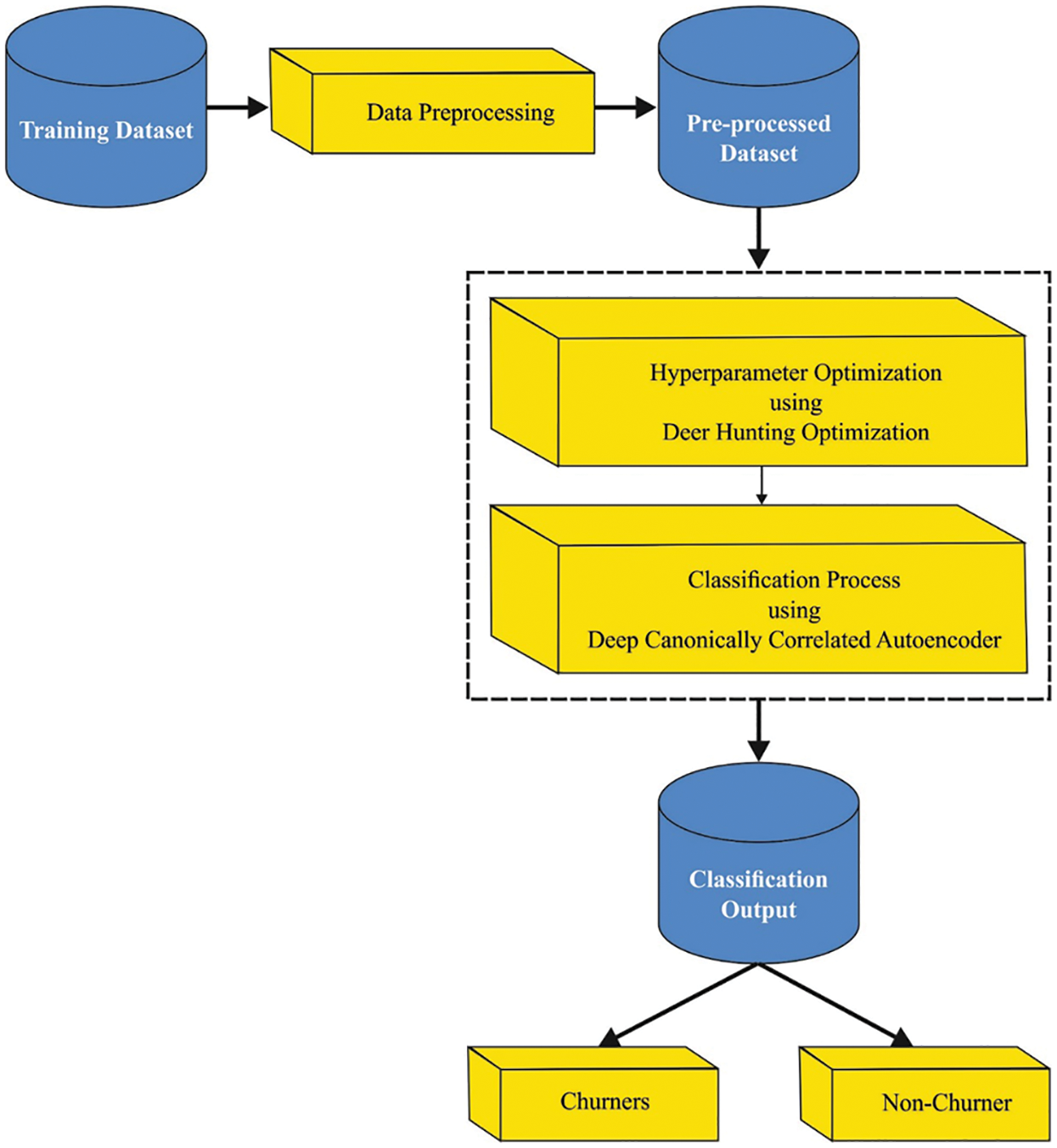
Figure 1: Workflow of O-DCCAEP model

2.1 DCCAE Based Classification

Once the customer data is pre-processed, they are fed into the DCCAE model to classify the churners or non-churner [16]. For tackling the limit of CCA technique, a deep neural network (DNN) is presented to canonical correlation analysis termed deep CCA (DCCA). The DCCA overcomes the constraint of CCA that couldn’t recognize complexity nonlinear relation. In DCCA, 2 DNNs f and g are learned nonlinear representations to every data set. The DCCA is accomplished by exploited the canonical correlation of 2 DNNs consequences f(X) and g(Y):

maxWf,Wg,U,V1Ntr(UTf(X)g(Y)TV)s.t.UT(1Nf(X)f(X)T+rI)U=IVT(1Ng(Y)g(Y)T+sI)V=IuiTf(Y)g(Y)Tvj=0,fori≠j(1)

Whereas N denotes the whole quantity of information, X and Y indicates the input matrices to 2 datasets, I denotes the identity matrix, f and g describes the nonlinear illustration of 2 DNNs with Wf and Wg parameters, U=[u1,…,uL] and V=[v1,…,vL] indicates the CCA direction that existing DNN results to topmost layer with L unit, and (rx,ry)>0 denotes the normalized parameter to covariance estimation. The DCCA is integrated with stacked autoencoder (SAE) for optimal representation of 2 datasets and a deep canonically correlated sparse autoencoder (DCSAE) which searches for deep network illustration of 2data sets for exploiting the canonical correlation among the 2 indifferent topmost feature, however, minimalizing the reform error of sparse AE. The DCSAE can be defined by:

minWf,Wg,U,V−1Ntr(UTf(X)g(Y)TV)+λN‖x(i)^−x(i)‖2+‖y(i)¯−y(i)‖2+αJKL(ρ‖ρj^)+βJKL(σ‖σ^k)(2)

where f and g imply the DNN employed to extract nonlinear features to each data set however, encode every input at the same time. U=[u1,…,uL] and V=[v1,…,vL] indicates the CCA direction that indicates the DNN results to topmost layer using L unit. x(i)^and y(i)^ suggests the reformation of input x(i) and input y(i) similarly JKL(⋅) denotes as JKL(ρ‖ρj^)=∑j=1Sρlogρρj^+(1−ρ)log1−ρ1−ρj^, whereas ρj^=1N∑i=1Nhj(x(i)) indicates the average activation of hidden layer j, correspondingly to JKL(σ‖σ^k).

2.2 DHOA Based Parameter Optimization

At last, the hyperparameter optimization of the DCCAE technique occurs utilizng the DHOA [17]. The main purpose of the projected DHOA approach is for detecting an optimal place for an individual for hunting the deer, it can be important for exploring the deer’s nature. It can contain special features which create difficult hunting for the predator. The distinct feature portrays visual power viz., 5 times superior related to humans. However, it required problem seeing green and red colors.

An important stage of method is the establishment of hunter population that is provided as:

Y={Y1,Y2,⋯,Yn}1<j≤n(3)

Assume n implies the total amount of hunters viz., the solution from the population Y.

Afterward, the beginning population, the deer place, and wind angles are essential parameters in defining an optimum hunter place were initializing. As the searching space is assumed as circles, the wind angle subsequently the circumference of circles.

θi=2πr(4)

In which r refers the arbitrary number utilizing a value from the range of [0,1] and i signifies the existing iteration. In order to moment, the position angle of deer was signified as:

ϕi=θ+π(5)

whereas θ signifies the wind angle.

While the place of optimal space was primarily unidentified, the method assumes the candidate solution nearby optimal viz., determined based on the fitness function (FF) as a better result. At this point, it regards the 2 outcomes, for instance, leadership place, Ylead, refers the primary optimal place of the hunter and successor place, Ysuccessor stands for the place of subsequent hunter.

(i) Propagation with leader place: then defining the optimal place all the individuals from the population tries to reach a better place and so, the process of upgrading the place begins. Accordingly, the surrounding nature was defined as:

Yi+1=Ylead−X⋅p⋅|L×Ylead−Yi|(6)

In which Yi stands for the existing iteration place, Yi+1 represents the subsequent iteration place, X and L imply the co-efficient vector and p signifies the arbitrary number establish supposing the wind speed, whereas the value range of [0–2]. The co-efficient vectors are computed as:

X=14loglog(i+1imax)b(7)

L=2⋅c(8)

Whereas imax denotes the maximal iteration, b indicates the variables that contain a value amongst −1 and 1 and c defines the arbitrary numbers from the interval of [0,1]. Fig. 2 showcases the flowchart of DHOA.

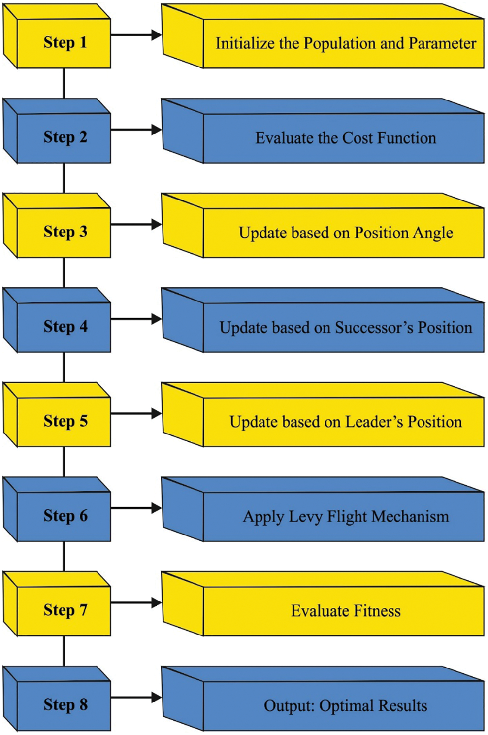
Figure 2: Flowchart of DHOA algorithm

In which (Y,Z) signifies the initial place of hunter that is upgraded dependent upon the prey place. The agent place was changed still an optimal place (Y∗,Z∗) has been obtained by adjusting L and X. All the hunters moved to leader place, once it can be effectual. However, the hunter remained from the existing place to ineffectual leader motion. The place upgraded subsequent in Eq. (7) if p<1, refers the discrete is move arbitrarily from every direction regardless of angle places.

(ii) Propagation with angle location: to enhance the searching space, the idea was extended by considering the angles placed from the upgraded rule. The angle evaluation was essential to define the hunter place therefore prey could not be attentive to attack and hereafter, the hunting method is effectual. The visualization angle of prey/deer were computed as:

ai=π8×r(9)

Based on the difference amongst visual and wind angles of deer, the variable was computed that is support for upgrading the angling place.

di=θi−ai(10)

Whereas θ signifies the wind angle. At that time, the angle places were upgraded to the subsequent iteration as:

ϕi+1=ϕi+di(11)

With assuming the angling place, the place was upgraded for implementation as:

Yi+1=Ylead−p⋅|cos⁡(v)×Ylead−Yi|(12)

In which A=ϕi+1, Yi∗ signifies the optimal place and p signify the arbitrary number.

(iii) Propagation using successor location: During the exploration step, an identical model in surrounding nature was changed by implementing the vector L. Therefore, the upgrading place was based on the successor place rather than initial optimal solution reached. This allows a global search that is offered as:

Yi+1=Ysuccessor−X⋅p⋅|L×Ysuccessor−Yi|(13)

whereas, Ysuccessor signifies the successor place of searching agent in the existing populations.

3  Results and Discussion

In this section, a detailed experimental validation of the O-DCCAEP model is performed using benchmark churn dataset [2] from telecommunication industry. The dataset involves 3333 instances with 483 coming under churner class and 2850 coming under non-churner class.

Fig. 3 demonstrates five confusion matrices produced by the O-DCCAEP model on five distinct runs. On run-1, the O-DCCAEP model has recognized 322 samples into churners and 2649 samples into non-churners class. Besides, on run-2, the O-DCCAEP model has recognized 111 samples into churners and 2845 samples into non-churners class. In addition, on run-3, the O-DCCAEP model has recognized 150 samples into churners and 2847 samples into non-churners class. Also, on run-4, the O-DCCAEP model has recognized 303 samples into churners and 2643 samples into non-churners class. At last, on run-5, the O-DCCAEP model has recognized 166 samples into churners and 2843 samples into non-churners class.

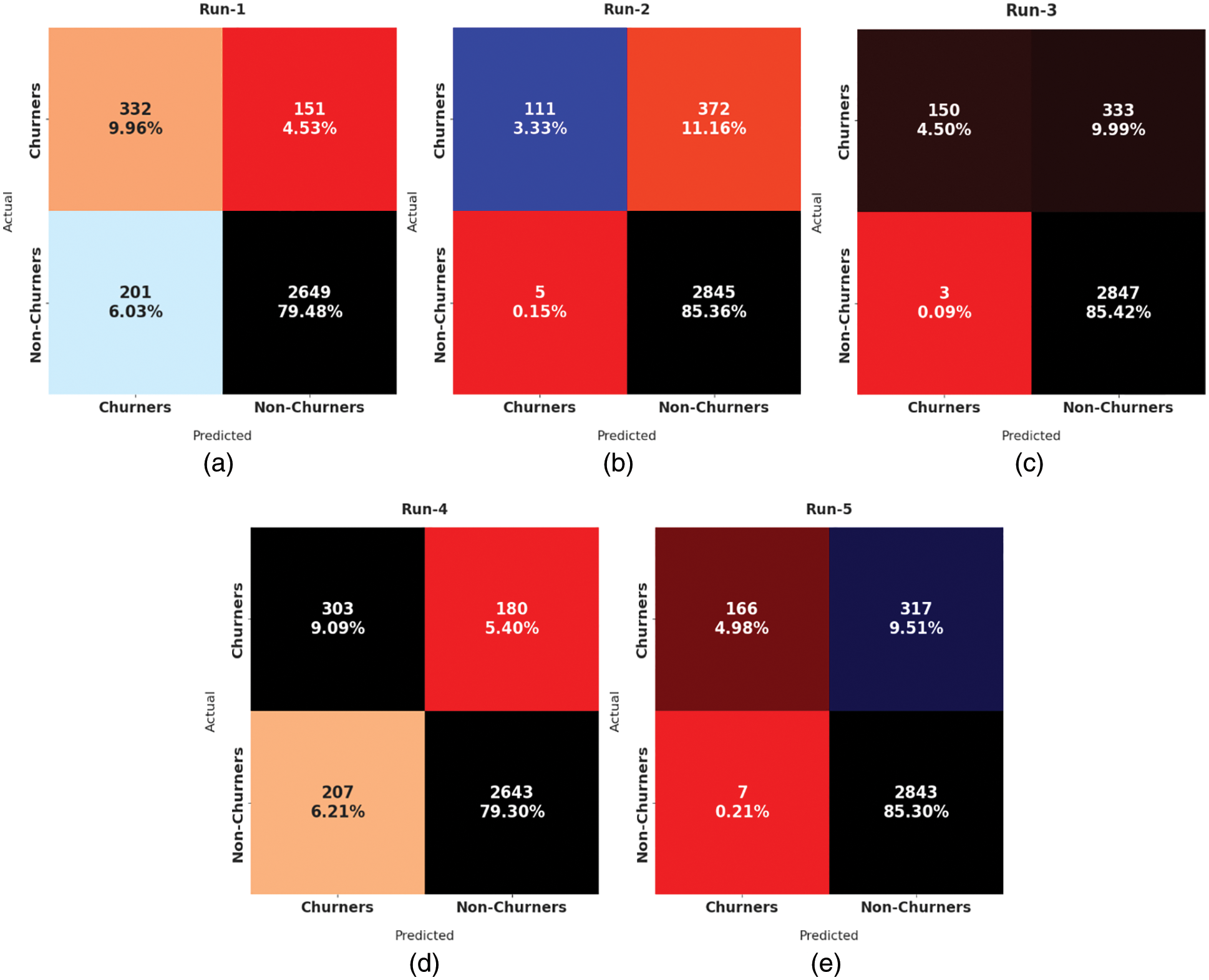
Figure 3: Confusion matrices of O-DCCAEP model

Tab. 1 and Fig. 4 report detailed CCP results of the O-DCCAEP model on the classification of churners and non-churners. The experimental results implied that the O-DCCAEP model has gained effectual outcomes with maximum CCP outcomes under distinct runs.

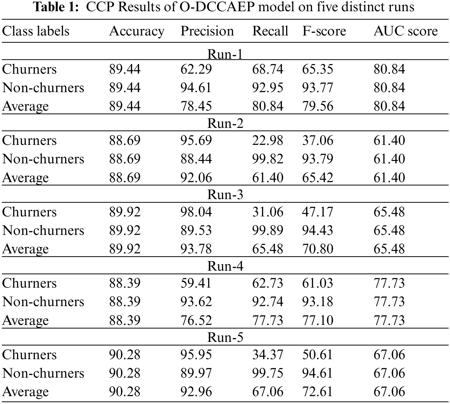
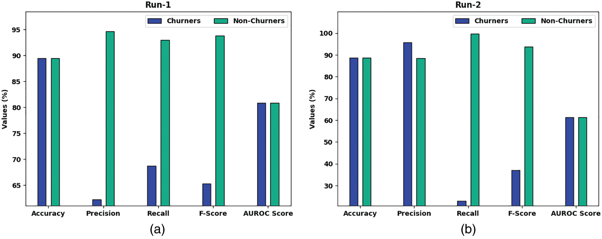
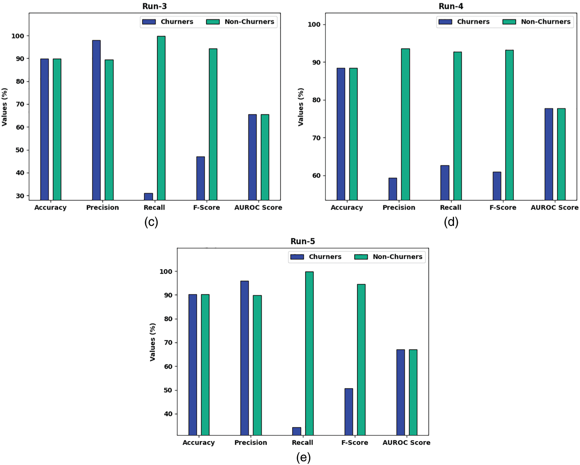
Figure 4: Overall CCP Results of O-DCCAEP model on five distinct runs

For sample, with run-1, the O-DCCAEP model has achieved average accuy,precn, recal, Fscore,and AUCscore of 89.44%, 78.45%, 80.84%, 79.56%, and 80.48% respectively. In addition, with run-2, the O-DCCAEP model has accomplished average accuy,precn, recal, Fscore,and AUCscore of 88.69%, 92.06%, 61.40%, 65.42%, and 61.40% respectively. Moreover, with run-3, the O-DCCAEP model has accomplished average accuy,precn, recal, Fscore,and AUCscore of 89.92%, 93.78%, 65.48%, 70.80%, and 65.48% respectively. Furthermore, with run-5, the O-DCCAEP model has gained average accuy,precn, recal, Fscore,and AUCscore of 90.28%, 92.96%, 67.06%, 72.61%, and 67.06% respectively.

Fig. 5 reports a detailed training accuracy (TA) and validation accuracy (VA) of the O-DCCAEP model on test data. The figure represented that the O-DCCAEP model has gained improved values of TA and VA.

Fig. 6 defines a comprehensive training loss (TL) and validation loss (VL) of the O-DCCAEP model on test data. The figure signified that the O-DCCAEP model has extended to least values of TL and VL.

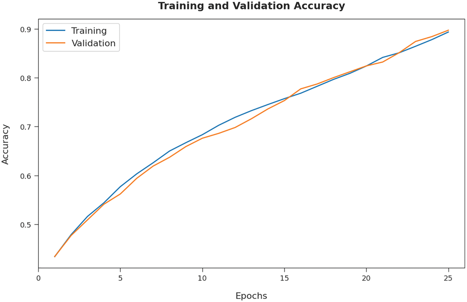
Figure 5: TA and VA analysis of O-DCCAEP model on five distinct runs

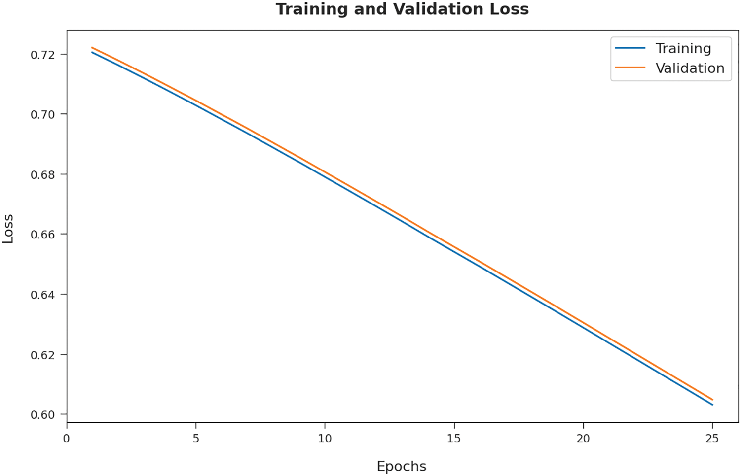
Figure 6: TL and VL analysis of O-DCCAEP model on five distinct runs

In order to exhibit the enhanced efficiency of the O-DCCAEP model, an extensive comparative examination is made in Tab. 2. Fig. 7 reports a detailed comparative study of the O-DCCAEP model with existing models in terms of accuy, recal, and precn. The results implied that the decision tree (DT) and k-nearest neighbor (KNN) models have accomplished least values of accuy, recal, and precn. Also, the logistic regression (LOR) method has reached somewhat higher values of accuy, recal, and precn. In line with, the Adaboost and CatBoost models have exhibited reasonable values of accuy, recal, and precn. However, the O-DCCAEP model has shown effectual outcome with maximum accuy, recal, and precn values of 89.44%, 78.45%, and 80.84% respectively.

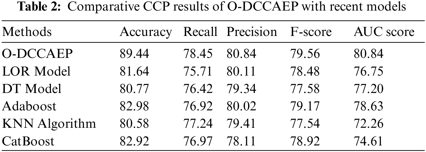
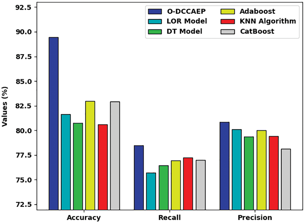
Figure 7: Comparative CCP results of O-DCCAEP model in terms of accuy, recal, and precn

Fig. 8 portrays a comprehensive comparative study of the O-DCCAEP model with existing models in terms of Fscore and. The experimental outcome demonstrated that the DT and KNN models have accomplished least values of Fscore and. Eventually, the LOR model has gained slightly enhanced values of Fscore and. Meanwhile, the Adaboost and CatBoost models have exhibited reasonable values of Fscore and AUC. However, the O-DCCAEP model has shown effectual outcomes with maximum Fscore and AUC values of 79.56% and 80.84% respectively. These results and discussion make sure the better outcomes of the O-DCCAEP model on CCP process.

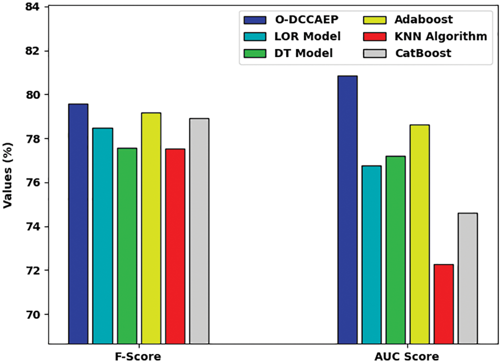
Figure 8: Comparative CCP results of O-DCCAEP model in terms of Fscore and AUC

4  Conclusion

In this study, a novel O-DCCAEP model was introduced to forecast customer churns in the telecommunication industry. The presented O-DCCAEP model encompasses three different processes. Initially, the pre-processing is carried out to transform the customer data into meaning format. Moreover, the DCCAE model is employed to classify the churners or non-churner. Furthermore, the hyperparameter optimization of the DCCAE technique takes place using the DHOA. The experimental evaluation of the O-DCCAEP technique is carried out against an own dataset and the outcomes highlighted the betterment of the presented O-DCCAEP approach on the recent approaches with maximum accuy, recal, and precn values of 89.44%, 78.45%, and 80.84% respectively. Thus, the O-DCCAEP model can be utilized for improvising the customer churn prediction performance. In future, advanced DL models can be utilized for feature selection process.

Funding Statement: This research work was partially supported by Chiang Mai University and Umm Al-Qura University.

Conflicts of Interest: The authors declare that they have no conflicts of interest to report regarding the present study.

This work is licensed under a Creative Commons Attribution 4.0 International License, which permits unrestricted use, distribution, and reproduction in any medium, provided the original work is properly cited.