DOI:10.32604/cmc.2022.030934
| Computers, Materials & Continua DOI:10.32604/cmc.2022.030934 | |
| Article |
Ensemble Machine Learning to Enhance Q8 Protein Secondary Structure Prediction
Computer Science Department, Faculty of Science, Minia University, 61519, Minia, Egypt
*Corresponding Author: Enas Elgeldawi. Email: enas.elgeldawi@mu.edu.eg
Received: 06 April 2022; Accepted: 11 May 2022
Abstract: Protein structure prediction is one of the most essential objectives practiced by theoretical chemistry and bioinformatics as it is of a vital importance in medicine, biotechnology and more. Protein secondary structure prediction (PSSP) has a significant role in the prediction of protein tertiary structure, as it bridges the gap between the protein primary sequences and tertiary structure prediction. Protein secondary structures are classified into two categories: 3-state category and 8-state category. Predicting the 3 states and the 8 states of secondary structures from protein sequences are called the Q3 prediction and the Q8 prediction problems, respectively. The 8 classes of secondary structures reveal more precise structural information for a variety of applications than the 3 classes of secondary structures, however, Q8 prediction has been found to be very challenging, that is why all previous work done in PSSP have focused on Q3 prediction. In this paper, we develop an ensemble Machine Learning (ML) approach for Q8 PSSP to explore the performance of ensemble learning algorithms compared to that of individual ML algorithms in Q8 PSSP. The ensemble members considered for constructing the ensemble models are well known classifiers, namely SVM (Support Vector Machines), KNN (K-Nearest Neighbor), DT (Decision Tree), RF (Random Forest), and NB (Naïve Bayes), with two feature extraction techniques, namely LDA (Linear Discriminate Analysis) and PCA (Principal Component Analysis). Experiments have been conducted for evaluating the performance of single models and ensemble models, with PCA and LDA, in Q8 PSSP. The novelty of this paper lies in the introduction of ensemble learning in Q8 PSSP problem. The experimental results confirmed that ensemble ML models are more accurate than individual ML models. They also indicated that features extracted by LDA are more effective than those extracted by PCA.
Keywords: Protein secondary structure prediction (PSSP); Q3 prediction; Q8 prediction; ensemble machine leaning; boosting; bagging
Proteins are essential to life, as they perform an enormous range of functions. They act as enzymes for catalyzing biochemical reactions. The collagen protein, for example, maintains the form of a cell as it is the main component of human skin, while the actin-myosin protein complex plays an important role in muscle contraction and thus macroscopic movement in living organisms. Proteins can function as molecular switches, altering the state of another protein [1]. In short, proteins are of vital importance to almost every biological process. Proteins are composed of linear chains of amino acids, which are linked by peptide bonds. The levels of protein structures are: the primary, secondary, tertiary and quaternary structures. The protein tertiary (native) structure is particularly interesting as it describes the 3D structure of the protein molecule, which reveals the functions of proteins which in turn helps in drug design and protein engineering.
Protein structure prediction (PSP) is very important in bioinformatics, medicine, theoretical chemistry, biotechnology and more. From the early days of biochemistry, the biochemists crucial concern was to know the protein structure (PS). In 1943, Fredrick has developed a way to spot amino acid sequence present in insulin [2]. However, this significant discovery didn't indicate whether an individual protein has multiple structures. In 1954, Anfinsen has found that amino acid sequence of a protein could fold into a 3D structure [3]. He has also investigated the amino acid sequence refolding and noticed that protein unfolded under extreme chemical environment, could refold back to 3D structure. Anfinsen has introduced a theory of folding, and said in his Nobel peace prize ceremony: “The native structure of protein is decided by the whole interactions between atomics and thus by the sequence of amino acids, in certain environment”. His theorem has provided an insight into the dilemma of PSP. The PSP terminology can be divided into two groups: (1) If proteins within the protein databank [4] have similarities in structure, then the target structure are often constructed by imitating the framework of the solved protein. This method is named template-based modeling [5]. However, this method cannot help in figuring out how proteins fold to their native structures. (2) If the protein structure has no similarities in the databank, the structure might be constructed from the amino acid sequence. This method is named ab initio [6], and it is the most difficult of all. This method depends on two components: energy function, which calculates the level of energy of every structure, and an enquiry procedure, which finds out the optimal structure with minimum energy within the search space. By the end of 2013, about 52 million-protein sequence were added to the protein sequence databank [7]. In addition, the amount of known PSs in the protein databank is about 90,000 [4].
The problem of the 3D structure prediction of a protein, based only on its primary structure (linear sequence of amino acids), is vitally important because the determination of protein structure experimentally is very expensive, while using the DNA sequencing to obtain protein sequences is cheap. Protein secondary structure is the most commonly predicted one-dimensional structure of proteins [8]. Protein secondary structure prediction (PSSP) has a significant role in the prediction of protein tertiary structure, as it bridges the gap between the protein primary sequences and tertiary structure prediction. There are three traditional experimental techniques employed to determine the secondary structure of proteins. These techniques are: X-ray crystallography, Nuclear Magnetic Resonance (NMR) spectroscopy, and Circular Dichroism spectrometry. As experimental methods are expensive and the number of proteins with known sequence is growing than the number of experimentally determined secondary structures, devising computational approaches for PSSP becomes increasingly urgent [9]. The prediction of protein secondary structure from only its amino acid sequence is a very difficult task. Protein secondary structures can be categorized into two classes: 3-state category, which includes: helix (H), strand (E), and coil (C); and 8-state category, which has been proposed by the DSSP (Define Secondary Structure of Proteins) program [10], includes: H (α-helix), G (310 helix), I (π-helix), S (bend), B (β-bridge), E (β-stand), T (β-turn), and L (loop or irregular). Protein sequence normally includes 2 kinds of sequence information: long-range interdependencies and local context [11,12]. The local contexts are essential for PSSP. Specially, the most valuable features to determine the secondary structure of an amino acid are the information about the secondary structure category of the neighbors of this amino acid. Also, long-range interdependency amongst different kinds of amino acids shows essential indicators for the type of a secondary structure. Predicting the 3 states and the 8 states of secondary structures from protein sequences are called the Q3 prediction and the Q8 prediction problems, respectively. Most of the methods of PSSP have been heavily concentrated on Q3 prediction. Although, Q8 prediction is complex and more challenging than Q3 prediction, in this paper, we focus on Q8 prediction, because the 8 classes of secondary structures reveal more precise structural information for a variety of applications than the 3 classes of secondary structures.
Ensemble learning (EL) techniques have shown great promise in improving the performance of classifier models in areas such as ML, data mining and pattern recognition. They possess a strength that has encouraged their use in several realistic classification problems. In fact, they supersede conventional ML methods in several applications and they have drawn the attention as a way to enhance the accuracy of prediction in highly complex problems. Many integration rules have been explored for developing EL techniques, but it is argued that no particular rule is better than others for devising an ideal decision [13]. EL has already been utilized in various applications such as face recognition, optical character recognition, gene expression analysis, computer-aided medical diagnosis, text categorization, etc. In fact, EL can be utilized anywhere ML methods can be utilized [14]. Ensemble learning methods, which have been broadly used for building improved classifier models, can be applied to PSSP [13,15–17]. In PSSP, the data (protein sequences) sequential nature demands particular ensembles. The known ensembles that depend on resampling or injecting randomness couldn't be used since the order of amino acids in protein sequences is important for consistent predictions and the success of prediction depends on the dependencies of amino acids. Thus, special devotion must be given to simple aggregation rule-based ensembles to fully investigate their ability to generalize in PSSP [13].
To this end, this paper presents a proposed ensemble ML approach for 8-state (Q8) PSSP. This approach employs two different ensemble methods, namely Bagging and Boosting. The ensemble members (base learners) considered for constructing the ensemble models are well known classifiers, namely Support Vector Machines (SVM), K-Nearest Neighbor (KNN), Decision Tree (DT), Naïve Bayes (NB), and Random Forest (RF), with two feature extraction techniques, namely PCA (Principal Component Analysis) and LDA (Linear Discriminate Analysis). Experiments have been conducted for evaluating the performance of single models as well as ensemble models, with PCA and LDA, in Q8 PSSP. To the best of our knowledge, the proposed approach is the first one to use EL for Q8 PSSP, as all the previous EL approaches have concentrated on Q3 prediction. This paper is organized as follows: related work is given in Section 2. Section 3 introduces the proposed ensemble machine learning approach for PSSP, and describes the methods and techniques employed in it, namely feature extraction techniques: LDA and PCA, the 5 ML algorithms: KNN, SVM, DT, RF, and NB, the two ensemble methods: Bagging and Boosting, and the models evaluation metrics. Section 4 presents the results of experiments that have been conducted to evaluate the presented models performance. Section 5 provides the conclusion of the work presented in this paper. Finally, future work is given in Section 6.
Today, machine learning algorithms is integrated in almost every scientific discipline such as networking [18–20], text analysis [21,22], image processing [23–30], cloud computing [31] and social networks [32,33]. This broad range of machine learning application disciplines is due to their promising predictive performance.
Since the 1950s, several techniques were developed for the prediction of secondary structure from amino acid sequences. Techniques extend from fields such as physical chemistry and biology to computer science and statistics [34–36]. This section presents a review of previous related work that applied ensemble ML techniques in PSSP.
Bittencourt et al. [15] have presented an empirical comparison of the performance of individual ML techniques (SVM, NB, KNN, Neural Network (NN) and DT) and ensemble techniques (boosting and bagging) in protein structural class prediction. They considered the prediction of the following classes: all-α, all-β, α + β, and α/β in addition to a class for the proteins that do not belong to any of the previous classes (small). The ensembles generated with bagging and boosting techniques utilized as base classifiers the single ML techniques DT, SVM and NN, and excluded KNN and NB, as the preliminary experiments showed that they are not suitable for the task. The experiments indicated that the results of ensemble techniques that utilized DT as the base classifier have shown consistent improvement.
Lin et al. [16] have applied a multi-SVM ensemble to improve the performance of PSSP. The SVM ensemble consisted of 2 layers; the first layer consisted of 3 SVMs network, where the winner is determined by winner-take-all; the second layer is a bagging ensemble network consisted of 5 classifiers, where its output is decided by majority voting. The classifiers were trained to predict three classes of PSS, which are H (helices), E (strands) and C (coil). The 7-fold cross-validation test on RS126 dataset showed that the multi-SVM ensemble achieved better Q3 accuracy of 74.98%.
Bouziane et al. [13] have investigated the effect of combining M-SVMs (Multi-class SVMs), KNNs, and ANNs to enhance globular proteins SSP. An ensemble technique that merges the outputs of 3 M-SVM, 2 Fead Forword NNs (FFNNs), and KNN classifiers has been used. Ensemble members are merged by 2 variations of the majority voting rule. To explore how much improvement the ensemble method can provide compared to the single classifiers that form the ensemble, the authors have applied the presented ensemble method on CB513 and RS126 datasets, by incorporating PSI-BLAST PSSM profiles as inputs. The experimental results indicated, in terms of Q3 accuracy, that performance of the proposed ensemble method was significantly better than that of the best single classifier. As can be seen from the above review, all the previous EL approaches have concentrated only on Q3 prediction.
This section describes the proposed approach for Q8 PSSP that uses ensemble machine learning to improve the accuracy of predicting protein secondary structures. The proposed approach to building an ensemble ML model for PSSP encompasses the following phases: (1) Data Preprocessing, (2) Features Extraction, (3) Data Splitting (Cross-validation method), (4) Ensemble Model Training, (5) Model Evaluation, and (6) Classification, as shown in Fig. 1. The phases of the proposed technique are explained in detail in the following subsections.

Figure 1: System model
Given a set of proteins, the first step in PSSP is to convert the set of sequences from strings of alphabetic characters in capital letters, corresponding to the twenty naturally occurring amino acids, into a feature-based representation. The training dataset used is CB6133, which is produced by PISCES CullPDB server [37]. This dataset includes 6128 non-homologous sequences, each of 39900 features. In the 6128 proteins, 500 proteins are training samples. The dataset is available for public use through literature [11]. Protein sequences in CB6133 have a similarity less than 25%, a resolution better than 3.0Å and an R factor of 1.0. The redundancy with test datasets was removed using cd-hit [38]. The 500 proteins × 39900 features were reshaped into 500 proteins × 700 amino acids × 57 features. The test dataset used is CB513, which is obtained from [11]. It is broadly used to evaluate the PSSP methods performance. It consists of 26143 α-helix, 1180 β-bridge, 17994 β-strand, 3132 310 helix, 30 π-helix, 10008 Turn, 8310 Bend, and 17904 Coil.
The extraction of the important features is an essential phase because irrelevant features often affect the classification efficiency of the ML classifier. The selection of features appropriately enhances classification accuracy and reduces the training time for the model. In the proposed ensemble ML approach for PSSP, features are extracted either by PCA (Principal Component Analysis) or LDA (Linear Discriminate Analysis) methods. These two techniques are described below.
3.2.1 Principal Component Analysis (PCA)
PCA is a multivariate technique. It is one of the most well-known techniques for the reduction of linear dimensionality [39]. PCA obtains the principal components in data by utilizing the covariance matrix and its eigenvectors and eigenvalues. These principal components are uncorrelated eigenvectors; each represents some percentage of variance in the data [40]. Let X = {x1, x2, …, xm} denotes a set of training data, xi represents a variable with dimensionality N, which stands for protein sequence in this work. The aim of PCA is two-fold: (a) get the highly significant information from X, and (b) reduce the dimensionality of X by preserving the significant information only. PCA is considered as an orthogonal projection of the initial N-dimensional data onto a new r-dimensional space (r < N), the projected data variance is the objective to be minimized [41]. The Initial letter of each notional word in all headings is capitalized.
3.2.2 Linear Discriminant Analysis (LDA)
LDA is a method for reducing dimensionality. It is utilized as a pre-processing stage in ML and pattern classification applications. LDA is primarily utilized in classification problems that have a categorical output variable. It can be used in binary and multi-class classifications. The LDA goal is to map the features in a high dimension space onto a low dimension space to overcome the dimensionality problem and decrease dimensional and resources costs [42]. The LDA model is comprised of the input data statistical attributes that have been computed for each class. In the case of having multiple variables, the same attributes are computed over the multivariate Gaussian. The predictions are made according to the probability that a new input dataset belongs to each class. The output class will be the one with the largest probability and accordingly the LDA does a prediction [42].
In data splitting phase, the cross-validation technique is used to split the training data set into testing data and training data. Cross-validation is a standard method used to estimate the performance of any ML algorithm on unseen data. One cycle of cross-validation includes splitting a sample of data into disjoint subsets, doing the analysis on one subset (named the training set), then validating the analysis on the other subset (named the testing set or the validation set). In our experiments, we have used 9-fold cross-validation. In this case, the dataset is split into 9 subsets: the first 8 are utilized to train the model, and the 9th is utilized to validate the model. This operation is repeated, allowing each of the 9 subsets of the split dataset an opportunity to be the test subset.
The proposed ensemble machine learning approach for Q8 PSSP combines two of the widely known ensemble techniques, namely Boosting [43,44] and Bagging [45], with five ML algorithms, namely K-Nearest Neighbor (KNN) [45], Support Vector Machines (SVM) [46], Decision Tree (DT) [47], Random Forest (RF) [48], and Naïve Bayes (NB) [49], as base learners.
EL is a ML technique in which several learners are trained to solve the same problem. Unlike conventional ML techniques, which attempt to learn one hypothesis from training data, ensemble techniques attempt to build hypotheses set and merge them for usage [49]. The two ensemble techniques used in our approach, namely Boosting and Bagging, are described below.
Boosting: The term “boosting” refers to a group of techniques that can convert weak models to strong models. The weak model is the one that has a considerable error rate, but the performance is not random (causing an error rate of 0.5 in the case of binary classification). Boosting gradually develops an ensemble by training each model with the same dataset but with adjusting the instances weights based on the last prediction error [38]. The basic concept is driving the models to concentrate on the instances that are misclassified. Then, the ensemble technique improves its efficiency by merging the trained weak models.
There are several variants of boosting. In this work, we use Adaptive Boosting (AdaBoost), which is a very famous boosting algorithm. It is proposed by Freund and Schapire [43]. Let X be the instance space, {–1, +1} be the set of class labels, and D = {(x1, y1); (x2, y2), …, (xN, yN)} is a given training data set, xi ∈ X and yi ∈ {–1, +1} (i = 1, …, N), (i = 1, …, N). AdaBoost works as follows: Firstly, it gives same weights to all the training instances. Let wt denotes the weights distribution at the t-th learning round. From wt and the training data set, the algorithm creates a base learner ht: X → {–1, +1} by invoking the base learner. Then, it utilizes the training instances to test ht, and increases the weights of the misclassified instances. Thus, a modified weight distribution wt+1 is gained. By invoking the base learner again with wt+1 and the training data set, AdaBoost creates another base learner. This process is iterated for M times, each iteration is named a round. The final learner is obtained by using weighted majority voting of the M base learners, where the learners' weights are established during the training process. Fig. 2 presents the pseudo-code of AdaBoost, which is adapted from [49].

Figure 2: AdaBoost algorithm
The function h : R → {0, 1} utilized in Algorithm 1 to calculate errm, the weight error rate of the mth classifier, is the Heaviside function, which is defined as:
Accordingly, since both hm(x_i) and yi take values in {–1, +1}, we have that
It is possible to utilize any ML algorithm as a base classifier with boosting, if it allows weights on the training set.
Bagging: Bootstrap Aggregation, which is referred to as Bagging [43], is a method that utilizes bootstrap sampling to decrease the variance and/or enhance the accuracy of some predictor. It may be utilized in regression and classification. It trains a number of base learners each from a distinct bootstrap sample by invoking a base learning algorithm. A bootstrap sample is found by subsampling with replacement the training data set, where the sample size equals to the training data set size.
Consider a size-N dataset Z = {z1, z2, …, zN}, where zi = (xi, yi), xi ∈ X and yi is a class label, in classification problems, or a real number, in regression problems. The main idea of bagging is to learn a set of B predictors (each from a bootstrap sample

Figure 3: Bagging algorithm
It should be noted that, in the above description of bagging and boosting methods, binary classification is considered for simplicity, but in this work, they are applied to Q8 PSSP, which is a multi-class classification problem. The Q8 secondary structure classes are: 310 helix (G), α-helix (H), π-helix (I), β-stand (E), β-bridge (B), β-turn (T), bend (S), and loop or irregular (L).
To assess the Q8 prediction performance of the presented ensemble models, we have used the following evaluation metrics: Accuracy, Recall, Precision, F-score, and AUC-ROC (Area Under the Curve - Receiver Operating Characteristics) curve.
This section presents the results of the experiments that we have conducted to evaluate the performance of the 5 individual predicting models, constructed using the 5 ML algorithms, KNN, SVM, DT, RF, and NB, and the ensemble models, constructed by combining each of the ensemble ML methods, bagging and boosting with each of the 5 ML algorithms, and the two feature extraction techniques, PCA and LDA, using cross validation tests, in Q8 PSSP. The individual predicting models and the ensemble models are applied to both CB6133 training dataset and CB513 test data.
4.1 Features Extracted by PCA and LDA
The number of important features that were extracted by both PCA and LDA equal 56 features for each amino acid (see Tab. 1).
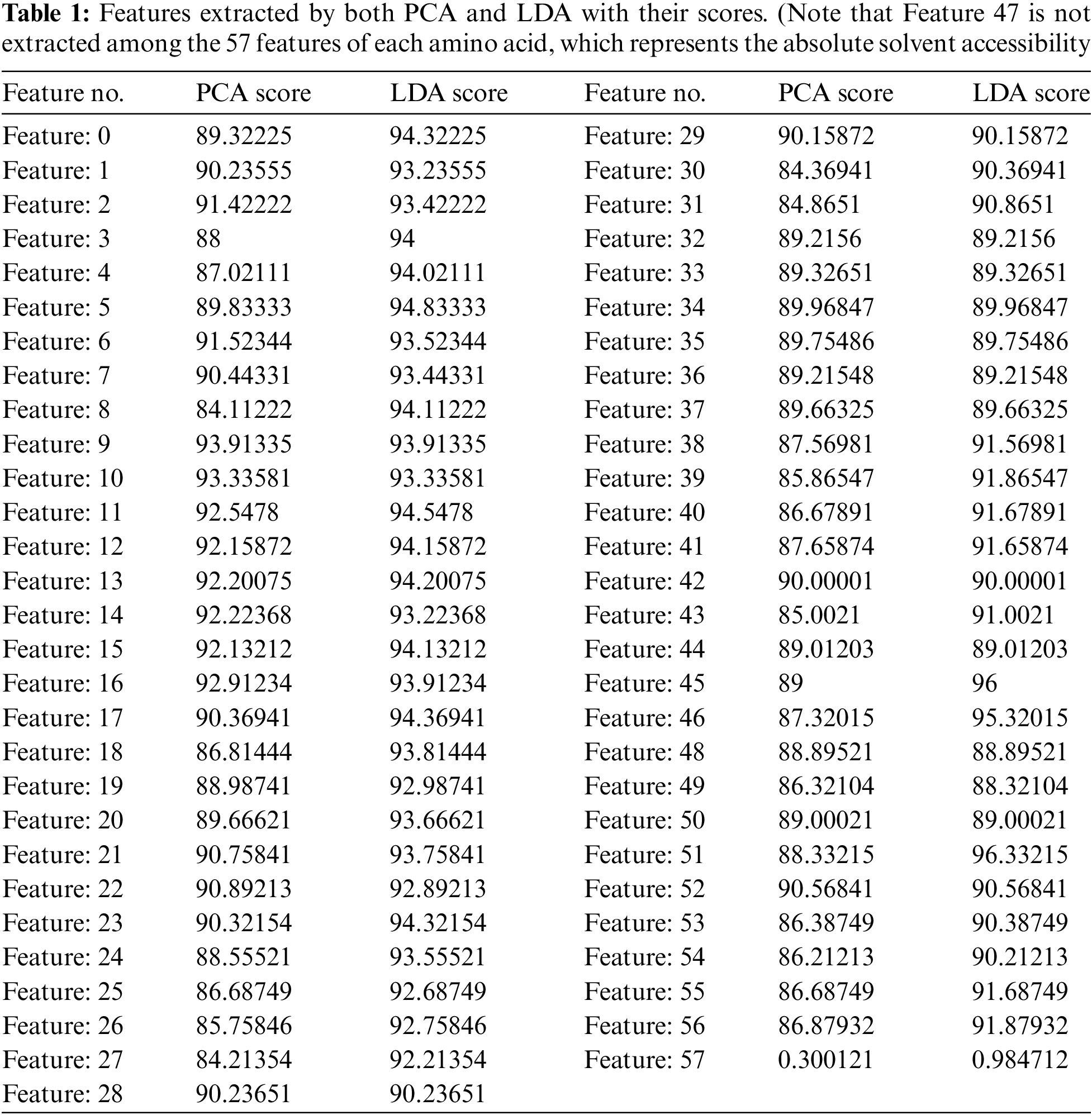
Tab. 1 shows the scores given to every feature, by PCA, according to the projected features variance, and by LDA, based on the distance between features. Among these 56 features, 22 represent the primary structure (20 amino acid, 1 unknown or any amino acid, 1 ‘NoSeq’ - padding), 22 represent the Protein Profile (same as primary structure), 2 represent N- and C-terminals, 1 represents relative solvent accessibility and 9 represent the secondary structure (8 possible states, 1 'NoSeq' - padding).
We have conducted 6 different experiments: In the first two experiments, we have applied the 5 ML algorithms to features extracted by PCA and LDA, respectively. In the next two experiments, we have applied the ensemble models, constructed by combining the bagging technique with each of the 5 ML algorithms, to features extracted by PCA and LDA, respectively. In the last two experiments, we have applied the ensemble models, constructed by combining the boosting technique (AdaBoost) with each of the 5 ML algorithms, to features extracted by PCA and LDA, respectively.
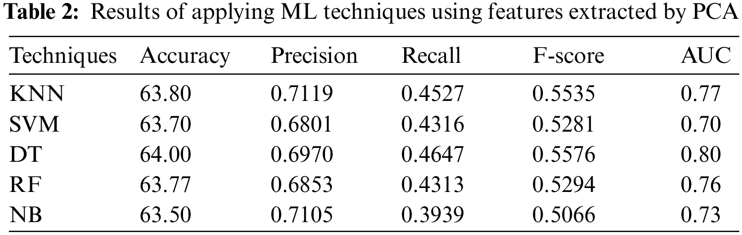
4.2.1 Experiment 1: Applying the ML Algorithms to Features Extracted by PCA
In the first experiment, the 5 ML algorithms have been applied to PSSP, utilizing the features selected by PCA. Tab. 2 displays the results of this experiment. Tab. 2 indicates that DT has the highest performance with accuracy = 64.00%, precision = 0.6970, Recall = 0.4647, F-score = 0.5576 and AUC = 0.80, while NB has the worst performance with accuracy of 63.50%, recall of 0.3939, and precision of 0.7105. The KNN technique has been applied with various number of nearest neighbors k = 1, 2, 3, 5, and 9. The best value was k = 1 that achieved accuracy of 63.80%, recall of 0.4527, precision of 0.7119, and AUC of 0.77. It is obvious from Tab. 2 that DT with PCA technique outperforms the other ML techniques, followed by KNN.
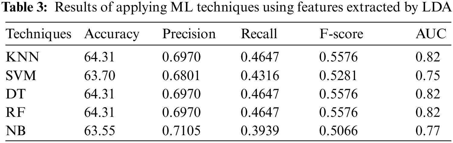
4.2.2 Experiment 2: Applying the ML Algorithms to Features Extracted by LDA
In the second experiment, features have been selected by LDA. Tab. 3 shows that DT, KNN (k = 1), and RF have the best performance with accuracy = 64.31%, precision = 0.6970, recall = 0.4647, F-score = 0.5576, and AUC = 0.82. The results shown in Tab. 3 indicate that DT, KNN, and RF with LDA technique outperform both SVM and NB.
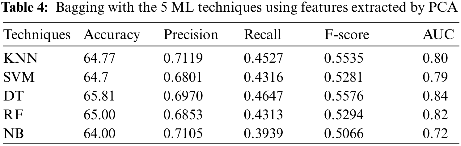
4.2.3 Experiment 3: Applying the Bagging Technique to Features Extracted by PCA
In the third experiment, the ensemble models, constructed by combining bagging with each of the 5 ML algorithms, with 9-fold cross-validation method, have been applied to PSSP, utilizing features extracted by PCA. Tab. 4 shows that DT has reached the best accuracy of 65.81%, recall of 0.4647, AUC of 0.84, and F-score of 0.5576, but KNN (k = 1) has reached the best precision 0.7119. NB has reached the worst accuracy of 64.00%, recall of 0.3939, AUC of 0.72 and F-score of 0.5066, while SVM has reached the worst precision of 0.6801. These results indicate that DT outperforms the other ML techniques when applying the bagging technique with them using features extracted by PCA.
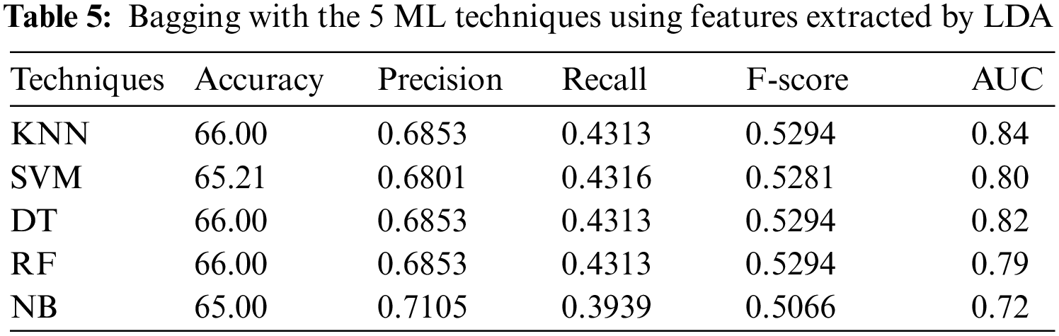
4.2.4 Experiment 4: Applying the Bagging Technique to Features Extracted by LDA
Tab. 5 shows the results when LDA is used, it can be seen that DT, KNN (k = 1) and RF have reached the best accuracy of 66.00% and F-score of 0.5294, while NB has reached the best precision of 0.7105, SVM has reached the best recall of 0.4316, and KNN (k = 1) has reached the best AUC of 0.84.
4.2.5 Experiment 5: Applying the Boosting Technique to Features Extracted by PCA
In the fifth experiment, the ensemble models, constructed by combining boosting with each of the 5 ML algorithms, with 9-fold cross-validation method, have been applied to PSSP, utilizing features extracted by PCA. From Tab. 5, we can see that RF achieved the best accuracy = 66.50%, recall = 0.4647, F-score = 0.5576, and AUC = 0.85, while DT achieved the best precision of 0.7119. In addition, Tab. 5 showed that SVM reached the lowest accuracy, precision, and AUC of 64.00%, 0.6801, 0.75, respectively, while NB reached the lowest recall and F-score of 0.3939 and 0.5066, respectively.

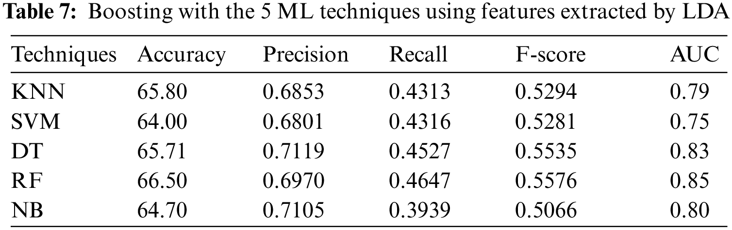
4.2.6 Experiment 6: Applying the Boosting Technique to Features Extracted by LDA
In the sixth experiment, the ensemble models, constructed by combining boosting with each of the 5 ML algorithms, with 9-fold cross-validation method, have been applied to PSSP, utilizing features extracted by LDA. Tab. 7 shows that RF achieved the best accuracy = 66.52%, recall = 0.4647, F-score = 0.5576, and AUC = 0.85, while DT achieved the best precision of 0.7119. In addition, Tab. 7 showed that SVM reached the lowest accuracy, precision, and AUC of 63.50%, 0.6801, 0.75, respectively, while NB reached the lowest recall and F-score of 0.3939 and 0.5066, respectively.
Tab. 8 summarizes the best values of the evaluation metrics: accuracy, recall, precision, F-score, and AUC, obtained in the presented experiments.

Fig. 4 shows a comparison between accuracy values of applying ML algorithms with and without ensemble learning using features extracted by PCA. This comparison indicates that, in general, the accuracy of the ML techniques has been improved by using ML ensemble learning as follows:
• The accuracy of KNN, RF and NB, were better with boosting than with bagging
• The accuracy of SVM and DT, were better with bagging than with boosting.

Figure 4: Accuracy values of applying ML algorithms with and without Ensemble Learning using features extracted by PCA
Fig. 5 shows a comparison between AUC values of applying ML algorithms with and without ensemble learning using features extracted by PCA. This comparison indicates that, in general, the AUC values of the ML techniques have been improved by using ML ensemble learning, as follows:
• The AUC values of RF and NB, were better with boosting than with bagging
• The AUC values of KNN, SVM and DT, were better with bagging than with boosting.

Figure 5: AUC values of applying ML algorithms with and without Ensemble Learning using features extracted by PCA
Fig. 6 shows a comparison between Accuracy values of applying ML algorithms with and without ensemble learning using features extracted by LDA. This comparison indicates that, in general, the accuracy of the ML techniques has been improved by using ML ensemble learning, as follows:
• The accuracy of KNN, SVM, DT and NB, were better with bagging than with boosting.
• The accuracy of RF was better with boosting than with bagging.

Figure 6: Accuracy values of applying ML algorithms with and without Ensemble Learning using features extracted by LDA
Fig. 7 shows a comparison between AUC values of applying ML algorithms with and without ensemble learning using features extracted by LDA. This comparison indicates that, in general, the AUC values of the ML techniques have been improved by using ML ensemble learning, as follows:
• The AUC values of DT, RF, and NB, were better with boosting than with bagging
• The AUC values of KNN and SVM were better with bagging than with boosting.

Figure 7: AUC values of applying ML algorithms with and without Ensemble Learning using features extracted by LDA
This paper presented a proposed ensemble machine learning approach to improve the performance of Q8 PSSP. In this approach, ensemble models for PSSP are constructed by combining two ensemble methods, namely Bagging and Boosting, with 5 ML algorithms, namely KNN, SVM, DT, RF, and NB, as ensemble members (base learners), and two feature extraction techniques, namely PCA and LDA.
We have conducted experiments for evaluating the performance of the 5 individual predicting models, constructed using the 5 ML algorithms, KNN, SVM, DT, RF, and NB, and the ensemble models, constructed by combining each of the ensemble ML methods, bagging and boosting, with each of the 5 ML algorithms, and the two feature extraction techniques, PCA and LDA, using cross validation tests on CB6133 training dataset and CB513 test data, in Q8 PSSP.
The experimental results indicated that:
• The best of all accuracy values, 66.52% and 66.50%, were obtained by Boosting with RF using features extracted by PCA and LDA, respectively.
• With features extracted by PCA, the accuracy of KNN, RF and NB, were better with boosting than with bagging, while the accuracy of SVM and DT, were better with bagging than with boosting.
• With features extracted by LDA, the accuracy of KNN, SVM, DT and NB, were better with bagging than with boosting, while the accuracy of RF was better with boosting than with bagging.
• The ML techniques KNN, DT, RF and NB achieved better accuracy when using features extracted by LDA than those extracted by PCA, while SVM achieved same accuracy when using both PCA and LDA.
• All bagging ensemble models achieved better accuracy when using features extracted by LDA than those extracted by PCA.
• Boosting with DT and NB achieved same accuracy when using both PCA and LDA, while boosting with KNN and RF achieved a little bit higher accuracy when using LDA than PCA and boosting with SVM achieved better accuracy when using PCA than LDA.
• For individual models, the best accuracy value was 64.31%, achieved by KNN, DT, and RF algorithms, when using features extracted by LDA.
• For bagging ensemble models, the best accuracy value was 66.00%, achieved with KNN, DT, and RF algorithms, when using features extracted by LDA.
• For boosting ensemble models, the best accuracy values were 66.52% and 66.50%, achieved with RF algorithm, when using features extracted by LDA and PCA, respectively.
These results clearly confirm that ensemble ML models are more accurate than individual ML models. They also indicate that features extracted by LDA are more effective than those extracted by PCA.
Funding Statement: The authors received no specific funding for this study.
Conflicts of Interest: The authors declare that they have no conflicts of interest to report regarding the present study.
1. L. Hunter, “Knowledge-based biomedical Data Science,” EPJ Data Science, vol. 1, no. 2, pp. 19–25, 2017. [Google Scholar]
2. P. Berg, “Fred Sanger: A memorial tribute,” Proceedings of the National Academy of Sciences, vol. 111, no. 3, pp. 883–884, 2014. [Google Scholar]
3. W. Sun, X. Chen, X. R. Zhang, G. Z. Dai, P. S. Chang et al., “A multi-feature learning model with enhanced local attention for vehicle re-identification,” Computers, Materials & Continua, vol. 69, no. 3, pp. 3549–3560, 2021. [Google Scholar]
4. PDB, “Protein data bank,” 2015. [Online]. Available: http://www.rcsb.org/pdb/home/home.do. [Google Scholar]
5. R. Adiyaman and L. McGuffin, “Methods for the refinement of protein structure 3D models,” International Journal of Molecular Sciences, vol. 20, no. 3, pp. 2301, 2019. [Google Scholar]
6. B. Berger and F. Leighton, “Protein folding in the hydrophobic-hydrophilic (hp) is np-complete,” Journal of Computational Biology, vol. 5, no. 1, pp. 27–40, 1998. [Google Scholar]
7. UniProt, “Protein sequence database,” [Online]. Available:, 2014. [Online]. Available: http://www.uniprot.org/. [Google Scholar]
8. W. Sun, G. C. Zhang, X. R. Zhang, X. Zhang and N. N. Ge, “Fine-grained vehicle type classification using lightweight convolutional neural network with feature optimization and joint learning strategy,” Multimedia Tools and Applications, vol. 80, no. 20, pp. 30803–30816, 2021. [Google Scholar]
9. J. Zhou, H. Wang, Z. Zhao, R. Xu and Q. Lu, “CNNH PSS: Protein 8-class secondary structure prediction by convolutional neural network with highway,” BMC Bioinformatics, vol. 19, no. 4, pp. 60–71, 2018. [Google Scholar]
10. W. Kabsch and C. Sander, “Dictionary of protein secondary structure: Pattern recognition of hydrogen-bonded and geometrical features,” Biopolymers, vol. 22, no. 12, pp. 2577–2637, 1983. [Google Scholar]
11. J. Zhou and O. Troyanskaya, “Deep supervised and convolutional generative stochastic network for protein secondary structure prediction,” ArXiv abs/1403.1347, 2014. [Google Scholar]
12. Z. Li and Y. Yu, “Protein secondary structure prediction using cascaded convolutional and recurrent neural networks,” ArXiv abs/1604.07176, 2016. [Google Scholar]
13. H. Bouziane, B. Messabih and A. Chouarfia, “Effect of simple ensemble methods on protein secondary structure prediction,” Soft Computing, vol. 19, no. 6, pp. 1663–1678, 2014. [Google Scholar]
14. Z. Zhou, “Ensemble learning,” in Encyclopedia of Biometrics, Springer, Boston, 2009. [Google Scholar]
15. V. G. Bittencourt, M. C. Abreu, M. C. de Souto and A. Canuto, “An empirical comparison of individual machine learning techniques and ensemble approaches in protein structural class prediction,” in Proc. of 2005 IEEE Int. Joint Conf. on Neural Networks, Montreal, Quebec, pp. 527–5311, 2005. [Google Scholar]
16. L. Lin, S. Yang and R. Zuo, “Protein secondary structure prediction based on multi-SVM ensemble,” in 2010 Int. Conf. on Intelligent Control and Information Processing, Dalian, China, pp. 356–358, 2010. [Google Scholar]
17. G. Zong, J. Liu, Y. Zhang and L. Hou, “Delay-range-dependent exponential stability criteria and decay estimation for switched hopfield neural networks of neutral type,” Nonlinear Analysis: Hybrid Systems, vol. 2010, no. 4, pp. 583–592, 2010. [Google Scholar]
18. S. S. Bacanli, F. Cimen, E. Elgeldawi and D. Turgut, “Placement of package delivery center for UAVs with machine learning,” in 2021 IEEE Global Communications Conf. (GLOBECOM), Madrid, Spain, pp. 1–6, 2021. [Google Scholar]
19. A. A. Radwan, T. M. Mahmoud and E. Elgeldawi, “Improving the efficiency of the flow deviation method for solving the optimal routing problem in a packet-switched computer network,” International Journal of Applied Mathematics, vol. 5, no. 2, pp. 171–187, 2001. [Google Scholar]
20. A. A. Radwan and E. Elgeldawi, “Solving the optimal routing problem in a packet-switching computer network using decomposition,” Egyptian International Journal, vol. 4, no. 9, pp. 1–13, 2003. [Google Scholar]
21. E. Elgeldawi, A. Sayed, A. R. Galal and A. M. Zaki, “Hyperparameter tuning for machine learning algorithms used for Arabic sentiment analysis,” Informatics, vol. 8, no. 4, pp. 79, 2021. [Google Scholar]
22. A. A. Sayed, E. Elgeldawi, A. M. Zaki and A. R. Galal, “Sentiment analysis for Arabic reviews using machine learning classification algorithms,” in Proc. of 2020 Int. Conf. on Innovative Trends in Communication and Computer Engineering (ITCE), Aswan, Egypt, pp. 56–63, 2020. [Google Scholar]
23. W. Wang, X. Huang, J. Li, P. Zhang and X. Wang, “Detecting COVID-19 patients in X-ray images based on MAI-nets,” International Journal of Computational Intelligence Systems, vol. 14, no. 1, pp. 1607–1616, 2021. [Google Scholar]
24. Y. Gui and G. Zeng, “Joint learning of visual and spatial features for edit propagation from a single image,” Visual Computer, vol. 36, no. 3, pp. 469–482, 2020. [Google Scholar]
25. W. Wang, Y. T. Li, T. Zou, X. Wang, J. Y. You et al., “A novel image classification approach via Dense-MobileNet models,” Mobile Information Systems, vol. 2020, no. 7602384, pp. 1–8, 2020. [Google Scholar]
26. S. R. Zhou, J. P. Yin and J. M. Zhang, “Local binary pattern (LBP) and local phase quantization (LBQ) based on Gabor filter for face representation,” Neurocomputing, vol. 2013, no. 116, pp. 260–264, 2013. [Google Scholar]
27. Y. Song, D. Zhang, Q. Tang, S. Tang and K. Yang, “Local and nonlocal constraints for compressed sensing video and multi-view image recovery,” Neurocomputing, vol. 2020, no. 406, pp. 34–48, 2020. [Google Scholar]
28. D. Zhang, S. Wang, F. Li, S. Tian, J. Wang et al., “An efficient ECG denoising method based on empirical mode decomposition, sample entropy, and improved threshold function,” Wireless Communications and Mobile Computing, vol. 2020, no. 2, pp. 1–11, 2020. [Google Scholar]
29. F. Li, C. Ou, Y. Gui and L. Xiang, “Instant edit propagation on images based on bilateral grid,” Computers, Materials & Continua, vol. 61, no. 2, pp. 643–656, 2019. [Google Scholar]
30. Y. Song, Y. Zeng, X. Y. Li, B. Y. Cai and G. B. Yang, “Fast CU size decision and mode decision algorithm for intra prediction in HEVC,” Multimedia Tools and Applications, vol. 76, no. 2, pp. 2001–2017, 2017. [Google Scholar]
31. E. Elgeldawi, M. Mahrous and A. Sayed, “A comparative analysis of symmetric algorithms in cloud computing: A survey,” International Journal of Computer Applications, vol. 182, no. 48, pp. 7–16, 2019. [Google Scholar]
32. E. Elgeldawi, A. A. Radwan, F. Omara and T. M. Mahmoud, “Detection and characterization of fake accounts on the pinterest social networks,” International Journal of Computer Networking, Wireless and Mobile Communication, vol. 4, no. 3, pp. 21–28, 2014. [Google Scholar]
33. A. A. Radwan, H. V. Madhyastha, F. Omara and T. M. Mahmoud, “Pinterest attraction between users and spammers,” International Journal of Computer Science Engineering and Information Technology Research, vol. 4, no. 1, pp. 63–72, 2014. [Google Scholar]
34. M. R. Girgis, E. Elgeldawi and R. M. Gamal, “A comparative study of various deep learning architectures for 8-state protein secondary structures prediction,” in Proc. of the Int. Conf. on Advanced Intelligent Systems and Informatics 2020, Cairo, Egypt, Springer, pp. 501–513, 2021. [Google Scholar]
35. W. Wardah, M. Khan, A. Sharma and M. A. Rashid, “Protein secondary structure prediction using neural networks and deep learning: A review,” Computational Biology and Chemistry, vol. 2019, no. 81, pp. 1–8, 2019. [Google Scholar]
36. G. Wang and R. L. Dunbrack, “Pisces: A protein sequence culling server,” Bioinformatics, vol. 19, no. 12, pp. 1589–1591, 2003. [Google Scholar]
37. W. Li and A. Godzik, “CD-hit: A fast program for clustering and comparing large sets of protein or nucleotide sequences,” Bioinformatics, vol. 22, no. 13, pp. 1658–1659, 2006. [Google Scholar]
38. C. Bishop and N. Nasrabadi, “Pattern recognition and machine learning,” Journal of Electronic Imaging, vol. 16, no. 4, pp. 1–16, 2007. [Google Scholar]
39. Z. M. Hira and D. Gillies, “A review of feature selection and feature extraction methods applied on microarray data,” Advances in Bioinformatics, vol. 2015, no. 112, pp. 1–13, 2015. [Google Scholar]
40. D. Zhang, L. Zou, X. Zhou and F. He, “Integrating feature selection and feature extraction methods with deep learning to predict clinical outcome of breast cancer,” IEEE Access, vol. 6, pp. 28936–28944, 2018. [Google Scholar]
41. P. Xu, G. N. Brock and R. S. Parrish, “Modified linear discriminant analysis approaches for classification of high-dimensional microarray data,” Computational Statistics & Data Analysis, vol. 53, no. 5, pp. 1674–1687, 2009. [Google Scholar]
42. Y. Freund and R. Schapire, “A decision-theoretic generalization of on-line learning and an application to boosting,” Journal of Computers and System Sciences, vol. 55, no. 1, pp. 119–139, 1997. [Google Scholar]
43. R. Schapire, “The strength of weak learnability,” Machine Learning, vol. 5, no. 2, pp. 197–227, 2005. [Google Scholar]
44. L. Breiman, “Bagging predictor,” Machine Learning, vol. 24, no. 2, pp. 123–140, 1996. [Google Scholar]
45. S. Jukic, M. Saracevic, A. Subasi and J. Kevric, “Comparison of ensemble machine learning methods for automated classification of focal and nonfocal epileptic eeg signals,” Mathematics, vol. 8, no. 9, pp. 1–16, 2020. [Google Scholar]
46. S. Abdullah, N. Rostamzadeh, K. Sedig, D. Lizotte, A. X. Garg et al., “Machine learning for identifying medication-associated acute kidney injury,” Informatics, vol. 7, no. 2, pp. 18, 2020. [Google Scholar]
47. L. Breiman, “Random forests,” Machine Learning, vol. 2004, no. 45, pp. 5–32, 2004. [Google Scholar]
48. H. Li and S. Misra, “Robust machine-learning workflow for subsurface geomechanical characterization and comparison against popular empirical correlations,” Expert Systems with Applications, vol. 177, no. 77, pp. 114942, 2021. [Google Scholar]
49. J. Wang, A. Zelenyuk, D. Imre and K. Mueller, “Big data management with incremental K-means trees-GPU-accelerated construction and visualization,” Informatics, vol. 4, no. 3, pp. 24, 2017. [Google Scholar]
 | This work is licensed under a Creative Commons Attribution 4.0 International License, which permits unrestricted use, distribution, and reproduction in any medium, provided the original work is properly cited. |