DOI:10.32604/cmc.2022.031514
| Computers, Materials & Continua DOI:10.32604/cmc.2022.031514 | |
| Article |
An Optimal Method for Supply Chain Logistics Management Based on Neural Network
1School of Engineering Technology, Al Hussein Technical University (HTU), Amman, 11831, Jordan
2Department of Medical Instrumentation Techniques Engineering, Dijlah University College, Baghdad, Iraq
3Department of Mechanical Engineering, College of Engineering, Taif University, Taif, 21944, Saudi Arabia
4Department of Electrical Engineering, University of Engineering and Technology, Peshawar, 814, Pakistan
5School of Computer Science and Engineering, Soongsil University, Seoul, Korea
*Corresponding Author: Bong Jun Choi. Email: davidchoi@soongsil.ac.kr
Received: 20 April 2022; Accepted: 20 May 2022
Abstract: From raw material storage through final product distribution, a cold supply chain is a technique in which all activities are managed by temperature. The expansion in the number of imported meat and other comparable commodities, as well as exported seafood has boosted the performance of cold chain logistics service providers. On the basis of the standard basic-pursuit (BP) neural network, a rough BP particle swarm optimization (PSO) neural network model is constructed by combining rough set and particle swarm algorithms to aid cold chain food production enterprises in quickly picking the best cold chain logistics service providers. To reduce duplicate information in the original data and make the input index more compact, the model employs rough set. Instead of using gradient descent to train the weights of the neural network, particle swarm optimization is utilized to ensure that the output results are not readily caught in local minima and that the network’s generalization capacity is improved. Finally, an example is presented to demonstrate the model’s validity and viability. The findings reveal that the model’s prediction error is 40.94 percent lower than the BP neural network model, and the prediction result is more accurate and dependable, providing a new technique for cold chain food production companies to swiftly pick the best cold chain logistics service provider.
Keywords: Supply-chain management; industrial enterprises; neural network; optimization
The growth in the consumer food quality and demand has brought both possibilities and problems to the development of cold chain logistics for fresh agricultural goods, but the rise in demand has also resulted in an increase in waste [1–5]. According to the China Food Industry Association, about US$10 billion of food is wasted each year due to inadequate cold chains during transportation. Therefore, for cold chain food production enterprises, choosing a reliable cold chain logistics service provider is a problem that must be faced to reduce the waste and maintain the sustainable development of enterprises [6–10]. Because of the unique nature of cold chain logistics, businesses should consider not only traditional factors like quality, customer satisfaction, and delivery reliability when selecting a service provider, but also cold chain logistics factors like transportation freshness rate, cold chain coverage rate, and so on [11–15]. It is required to develop a thorough selection evaluation index system and scientific evaluation technique in order to completely assess the quality of cold chain logistics service providers.
Because a dependable service provider is critical to a company’s success, academics both at home and abroad have conducted extensive research on service provider selection [16–18]. References [19,20] provided essential anticipation of supplier evaluation indicators in the development of the evaluation index system. They compiled 23 criteria for evaluating suppliers is ranked in order of importance. Reference [21] used five primary indicators, such as cold chain business level, service quality, facilities, equipment, and two secondary indicators, such as cold chain logistics temperature compliance rate and product loss rate to create an evaluation index for the selection of agricultural cold chain logistics service providers. However, there is no scientific evaluation procedure to check the reasonableness of the evaluation index after it has been built.
In terms of evaluation methods, reference [22] used the analytical hierarchical process (AHP) method to establish a comprehensive evaluation model for cold chain logistics suppliers, but the method of constructing a judgment matrix by expert scoring is relatively subjective, and the premise is that there is no interdependence between factors at all levels and the model is too idealistic. Considering that the evaluation indicators are often interdependent and complex, reference [23] used the analytical network process (ANP) method to build a logistics service provider selection model, but the solution process of this model requires a lot of computation, and the determination of the comparison matrix also requires the author to have accurate judgment and extensive experience. In order to avoid the shortcomings of a single evaluation model, most scholars tend to use several models in combination to utilize their respective advantages. For example, reference [24] ranked cold chain logistics service providers using a fuzzy AHP and Technique for Order of Preference by Similarity to Ideal Solution (TOPSIS) hybrid model. The addition of the TOPSIS method avoids the problem that the AHP method is too simple to sort the evaluation indicators. Reference [25] adopts the method of combining ANP and Markov chain, and introduces a supplier selection method oriented to customer needs, which provides a new idea for supplier selection. In addition, there are non-radial Data Envelopment Analysis (DEA) [26], AHP + factor analysis + fuzzy comprehensive evaluation [27] methods and so on.
With the deepening of research and the popularization of computer technology, most scholars have begun to use intelligent algorithms to evaluate and select suppliers. Among them, the artificial neural network (ANN) has unique advantages in dealing with the complex relationship between the supplier evaluation indicators with its unique nonlinear adaptive information processing capability. The use of a BP neural network in supplier selection was introduced in reference [28], which may better eliminate subjective impact and evaluation ambiguity. The classic BP neural network approach, on the other hand, has issues such as low adaptation to data other than training and produces a local minimum as a consequence. As a result, several researchers have worked to enhance the neural network method. Reference [29], for example, employed a genetic algorithm to optimize a neural network to choose ship providers. The PSO algorithm was utilized to optimize the neural network and the principal component analysis approach was employed to simplify the input indications in reference [30]. The wavelet neural networks were employed to choose providers in reference [31], and rough set theory was applied to reduce the input indications. The neural network and grounded theory were merged in reference [32]. The BP neural network was integrated with the DEA cross-evaluation model, among other things, in reference [33], which enhanced the neural network’s performance to some extent.
After sorting through the previous research findings, this paper employs the particle swarm algorithm to optimize the BP neural network for selecting the cold chain logistics service provider, which not only compensates for the BP neural network algorithm’s tendency to fall into the local minimum value, but also eliminates the subjective influence of factors, making the evaluation selection results more objective and fair. The rough set theory, which is simple to apply and does not alter the information contained in the data, is used to minimize the amount of input indicators in order to overcome the problem of poor network generalization ability caused by redundant input indications. Finally, an example is used to demonstrate the algorithm’s viability.
The cold chain food production firms can accurately pick and assess cold chain logistics service providers is determined by whether the evaluation index method is scientific, thorough, and effective. Because various organizations have distinct demands for logistics service providers, the selection criteria are also variable. The companies whose products must be frozen and delivered should assess not just typical logistics service providers’ quality, cost, service, and other indicators, but also the particular skills and levels. As a result, this study uses dairy cold chain logistics service providers as an example, discusses [34] in depth, and creates an evaluation index system for dairy cold chain logistics service provider selection. Fig. 1 depicts the relevant indications.
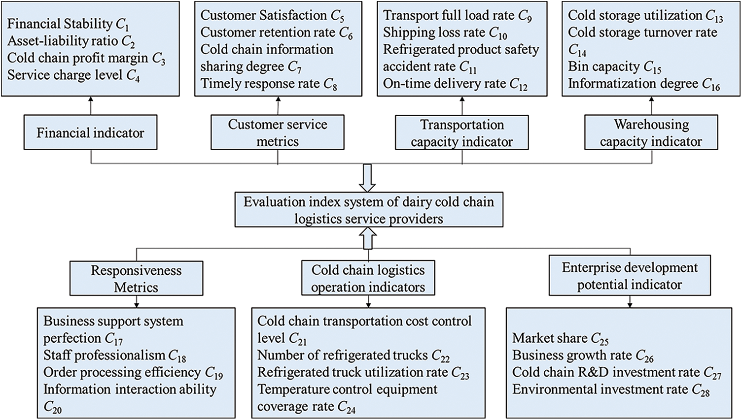
Figure 1: System model of index evaluation
The financial indicators are the embodiment of the cold chain logistics service provider’s business performance in Fig. 1, showing the company’s capacity to continue production and operations. The capacity of cold chain logistics service providers to fulfil client demands is measured by the customer service index. Because transportation and storage are the two fundamental tasks of logistics, transportation and warehousing capacity indicators provide the foundation for assessing cold chain logistics service providers’ basic competitiveness. Because of the perishable nature of refrigerated items, cold chain logistics service providers must process orders quickly and the prompt response rate represents the capacity of cold chain logistics services to perform tasks issued by businesses on time. The ability of cold chain logistics service providers in terms of cost management and hardware level is measured at the operating level. The indicator of enterprise development potential refers to the ability of the enterprise to create value in the future which represents the future development prospects of the enterprise. This metric is used to assess the likelihood of long-term collaboration with cold chain logistics service providers. All secondary indicator data is sourced from cold chain logistics service providers’ historical data.
The model used by cold chain logistics service providers is upgraded based on the properties of the BP neural network. The PSO method is integrated with the BP neural network in this article, and the rough set theory difference moment is applied. The new matrix technique reduces the input index, and the proposed model enhances the original BP neural network model in two ways.
1) It is frequently important to simplify the input indications and erase redundant information in order to increase the accuracy of the BP neural network’s prediction outputs. The principal component analysis is now the most popular approach for simplifying the input indicators according to study findings on service provider selection. This approach uses the concept of dimensionality reduction to reduce a large number of linearly connected indicators to a small number of unrelated indications with the goal of preserving as much information as possible. That is, the principal component is a linear combination of the original indicators. The correlation between the indicators is, however, a condition of the principal component analysis approach. For starters, this approach is incapable of dealing with nonlinear situations. Second, the degree of correlation between the indicators is either too high or too low, affecting the accuracy of the results. The rough set theory can remove the unnecessary data from the original data without changing the information stated in the data, and it doesn’t require any prior knowledge beyond the data set to be processed. When it comes to examining index reduction, the set theory offers greater advantages.
2) Because the BP neural network modifies the connection weights using the gradient descent approach, the network’s adaptability to new input is restricted, and the output result is a local minimum value. Researchers are progressively combining bionic intelligence algorithms with neural networks as research progresses. Because the intelligent algorithm has excellent global convergence and durability, combining the two can increase the neural network’s prediction accuracy and generalization mapping ability. The Genetic algorithm (GA), as the most extensively used evolutionary algorithm, may be used to solve a variety of complicated issues, but the optimization process is difficult to regulate because there are too many parameters to control in the connections of selection, crossover, and mutation. When dealing with optimization issues, the PSO algorithm’s operation is generally straightforward, does not require the function’s gradient information or other prior knowledge, and may be substantially parallelized. As a result, instead of using the genetic method to train the weights and thresholds of the neural network, this research employs the particle swarm approach. As a result, the neural network’s performance is improved. Fig. 2 depicts the proposed PSO-BP neural network algorithm design concept.
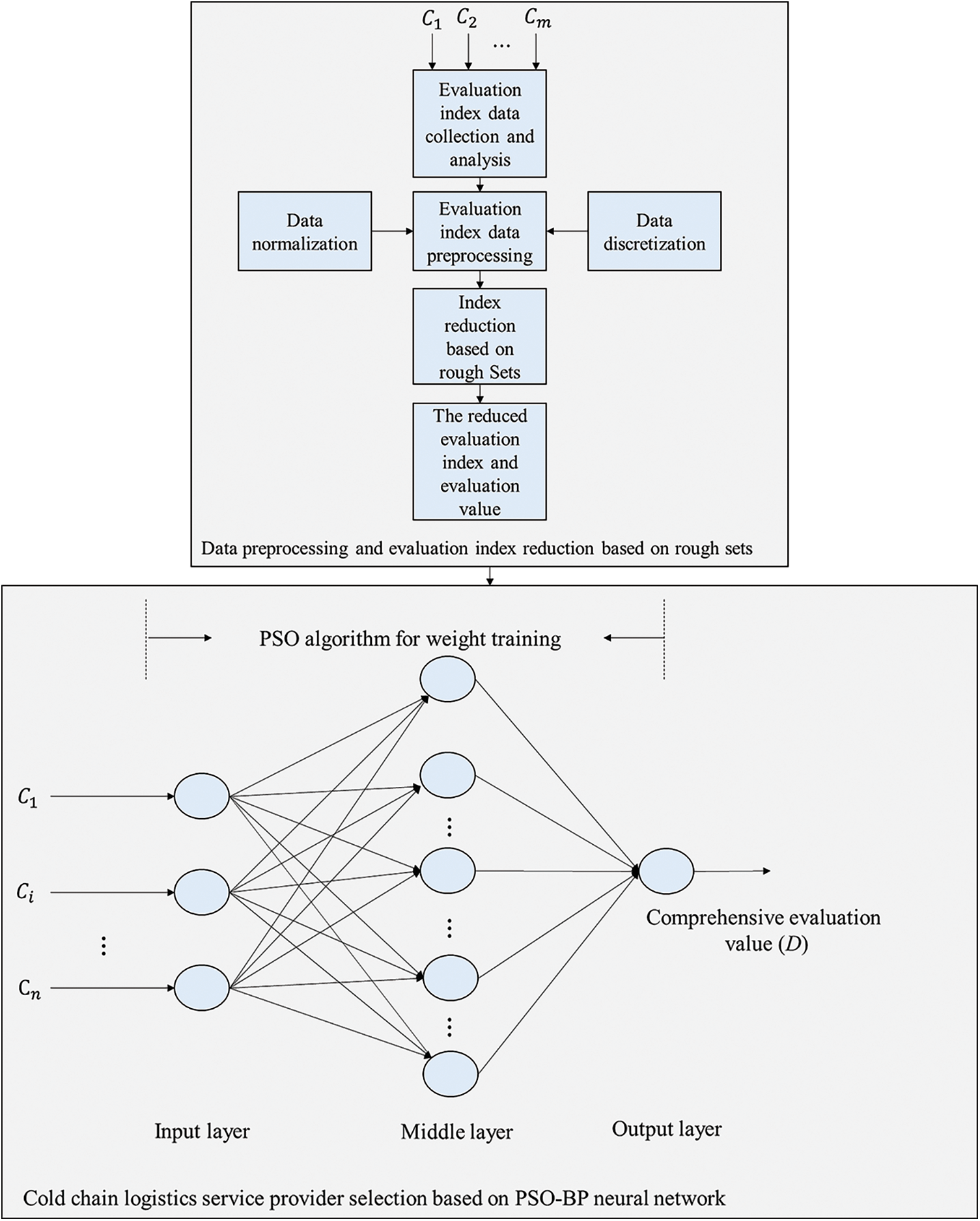
Figure 2: Proposed algorithm model
The proposed approach works by first preprocessing the neural network’s input indications using rough sets. That is, normalize and discretize the evaluation index data to create a decision table, then minimize the evaluation index and eliminate the redundant indexes using the difference matrix improved technique. The reduced evaluation index is then used to learn and train the PSO-BP neural network. At this point, the PSO algorithm will optimize the BP neural network’s initial weights and thresholds as particles, and the BP network will be trained using the optimized weights and thresholds.
Step 1: The evaluation index data and complete scores of each cold chain logistics service provider are normalized and discretized. The expression is as follows:
where the lower triangular matrix of the difference matrix is denoted by
Among them, c is the service provider condition attribute value;
Step 2: The single element in the difference matrix is the kernel of attribute reduction, and the element containing the kernel attribute in the difference matrix is changed to 0.
Step 3: For all the elements in the difference matrix whose value is “non-empty set”, establish the corresponding conjunctive normal form L, and then convert the conjunctive normal form L into the disjunctive normal form L’.
Step 4: Produce the reduction result. Each disjunctive normal form conjunction is an attribute reduction, and the attributes included in each conjunction form a conditional attribute set.
Step 5: Input the reduced evaluation index into the proposed model.
Step 6: Calculate the number of neurons in the neural network’s input-hidden-output layer.
Step 7: Determine the number of particles m and the position of each particle is
Step 8: Calculate the fitness value J for each particle.
where N is the number of samples in the training set; E is the number of output neurons is;
Step 9: If
Step 10: If
Step 11: Update the position and velocity of the particle.
The speed update formula is expressed as:
The location update formula is expressed as:
where
Step 12: Use the maximum speed value to limit the particle update speed, and use the boundary position to limit the particle update position.
If
Among them,
Step 13: Check to see whether the following requirements are met: 1) The error is within the given error accuracy; 2) the maximum number of iterations permitted has been reached. The iteration finishes if one of the requirements is met. Otherwise, return to step 8.
Step 14: Create the best possible solution. After iteration, the value of is the global optimal solution, which can be used to train and learn the BP neural network by adjusting the weight and threshold. Fig. 3 depicts the flowchart of the proposed method.
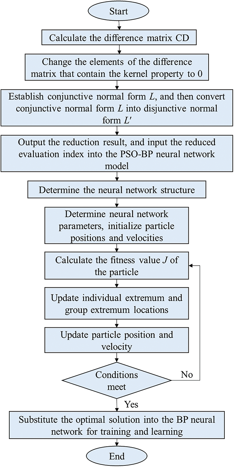
Figure 3: Proposed algorithm flowchart
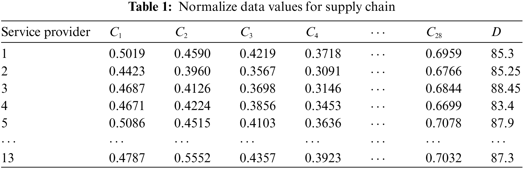
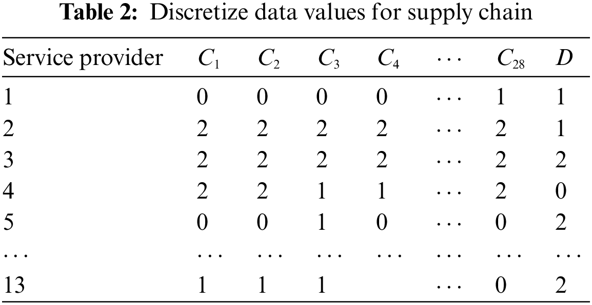
Milk, yoghurt, and ice cream are among the items produced by a huge dairy company. To meet the increased market demand, the business plans to collaborate with one of five alternative cold chain logistics service providers. Following further investigation and analysis of these five cold chain logistics service providers, relevant data is obtained, based on the data of 13 cold chain logistics service providers who have previously collaborated (8 for training service providers, 5 for testing service providers quotient), using the rough PSO-BP neural network model proposed in this paper for selection. Because the units of the original data are varied, the original data of 13 cold chain logistics service providers is first adjusted to remove dimensional effect. Tab. 1 shows the service provider data (C1∼C28) after normalization, as well as the company’s comprehensive score (D) for the service provider.
4.1 Evaluation Index Reduction Based on Improved Algorithm of Rough Set Difference Matrix
Because rough sets can only cope with discretized data, the data in Tab. 1 is discretized using the equidistant approach. After discretization, it is divided into 3 grades, and the grade classification standard is as follows. Take the minimum and maximum values in the jth value and label them as
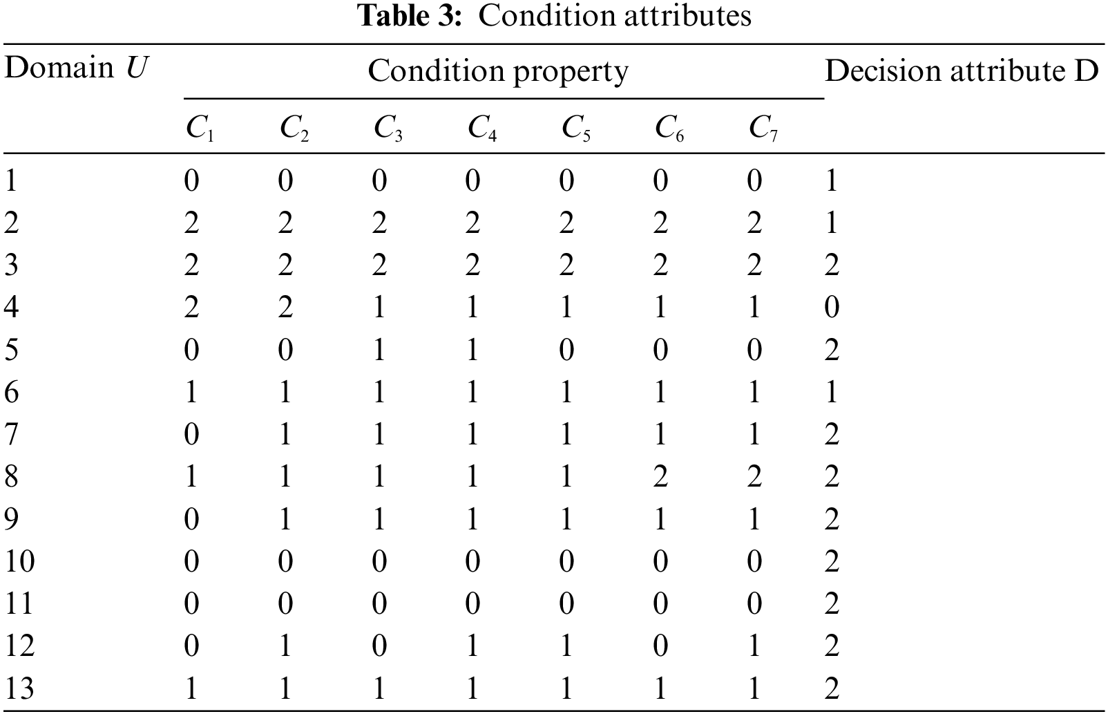
The 28 evaluation indexes are reduced by the improved difference matrix algorithm. For the convenience of calculation, the 28 evaluation indexes are divided into 4 groups, and the evaluation indexes are reduced respectively.
The universe of discourse in Tab. 3 represents the 13 cold chain logistics service providers that have cooperated with each other, the condition attribute
4.1.1 Difference Matrix Calculation
According to the two-dimensional decision table, calculate the difference matrix
4.1.2 Evaluation Index Reduction
According to the difference matrix
From the matrix
The attribute reduction results of evaluation indicators
The attribute reduction process of evaluation indicators
4.1.3 Evaluation Index System After Calculation Reduction
The results of attribute reduction
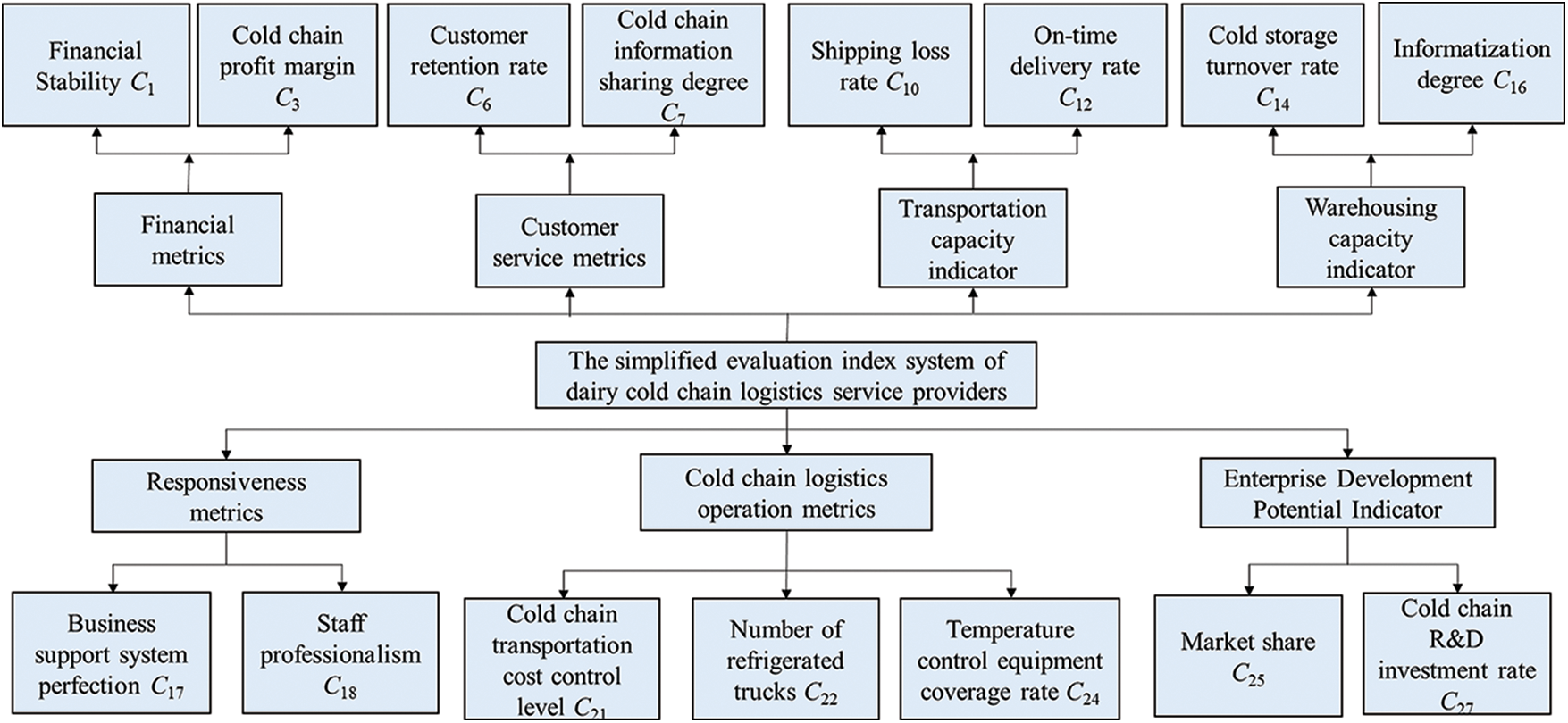
Figure 4: Logistics model with reduced index
4.2 Supplier Selection Based on PSO-BP Neural Network
4.2.1 Algorithm Parameter Settings
The proposed algorithm was simulated in MATLAB R2018a. The input node is 13 (the number of cold chain logistics service providers), the output node is 1 (the cold chain logistics service provider’s comprehensive evaluation value), and the hidden layer’s number of neurons is 9. The PSO algorithm has a population size of 40, an acceleration constant of
To predict the comprehensive evaluation results of cold chain logistics service providers, the normalized data of 13 cold chain logistics service providers was imported into the proposed neural network for training, and 8 cold chain logistics service providers were randomly selected as the training set and 5 cold chain logistics service providers as the test set. A comparison study is carried out in two parts to assess the efficiency of the model in this research. Comparing the BP neural network algorithm to the rough-BP neural network algorithm is the first step. Second, the results of the rough PSO-BP neural network method are compared to those of the rough-BP neural network algorithm.
4.2.2 Comparison of Forecast Results
The 28 assessment indicators are first input into the BP neural network without rough set reduction, and the network training curve is shown in Fig. 5. The 15 assessment indicators are then fed into the BP neural network after preliminary set reduction, and the network training curve is illustrated in Fig. 6. The comparison of training outcomes before and after attribute reduction is shown in Tab. 4.
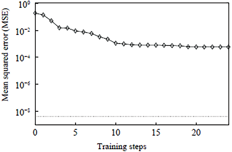
Figure 5: Comparison of the mean squared error training of the original data

Figure 6: Comparison of mean squared error with attribute reduction
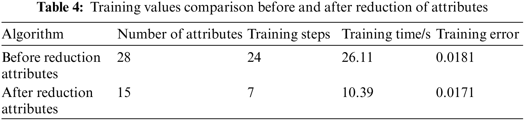
Figs. 5 and 6 and Tab. 4 indicated that, after rough set attribute reduction, the number of training steps in the BP neural network is decreased from 24 to 7, and the training time is lowered from 26.11 to 10.39 s. Before attribute reduction, the training error was 94.48%. The number of training steps and training duration of the BP neural network are decreased as a result of rough set removing redundant features across indicators, however rough set as a data processing technique does not increase prediction accuracy.
The 15 evaluation indicators are input into the PSO-BP neural network and the BP neural network, respectively, after attribute reduction by rough set, and the data of 13 cold chain logistics service providers is trained, and the resultant prediction results are displayed in Figs. 7 and 8, respectively.
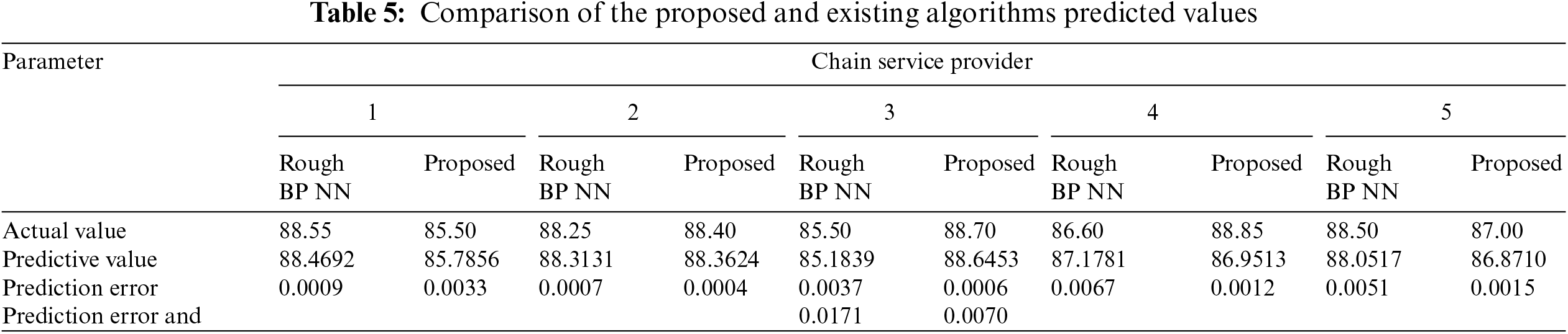
The suggested approach has a better fitting impact on the comprehensive assessment findings of cold chain logistics service providers, as shown in Figs. 7 and 8. The true value, expected value, and magnitude of prediction error of the comprehensive assessment findings of cold chain logistics service providers generated by the two algorithms may be shown in Tab. 5. Due to the addition of particle swarm optimization, the prediction error sum of the algorithm in this paper is 40.94% of the prediction error sum of the rough-BP neural network algorithm, which improves the prediction accuracy of the algorithm.
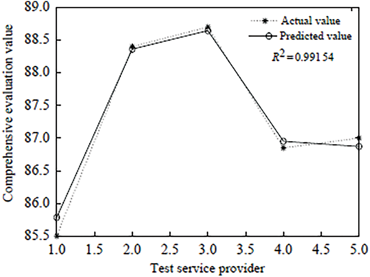
Figure 7: Comprehensive evaluation value of test service providers with rough PSO-BP NN
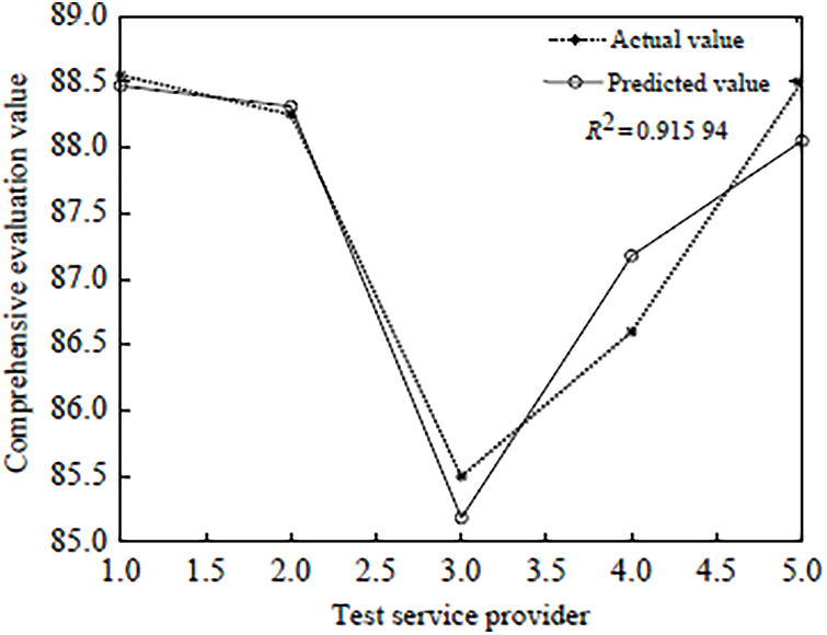
Figure 8: Comprehensive evaluation value of test service providers with rough BP NN
The comparison between the BP neural network algorithm and the rough-BP neural network algorithm, as well as the comparison between the rough PSO-BP neural network algorithm and the rough-BP neural network algorithm shows that after the rough set reduces the attributes of the evaluation indicators, the training samples and neural network structure are improved and the neural network training speed is improved, but the prediction accuracy is not improved. The use of a PSO and BP neural network together increases the neural network’s generalization ability and the algorithm’s accuracy. Finally, the proposed method can increase the prediction accuracy while lowering network running time, allowing the cold chain food production firms to correctly and rapidly pick the best cold chain logistics service provider.
4.2.3 Service Provider Selection for Cold Chain Logistics
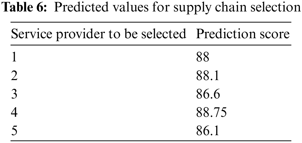
Input the data of the five cold chain logistics service providers to be selected into the trained PSO-BP neural network model, and select the best partner according to the predicted comprehensive evaluation value.
According to Fig. 9 and Tab. 6, it can be seen that the predicted score ranking of cold chain logistics service providers is: Service Provider 4 > Service Provider 2 > Service Provider 1 > Service Provider 3 > Service Provider 5. Therefore, the dairy product manufacturer can choose cold chain logistics service provider 4 as its partner.

Figure 9: Predicted composite score
This paper proposed a rough PSO-BP neural network algorithm that employs a rough set correlation theory to remove the redundant information from the original data in the selection of cold chain logistics service providers, resulting in a more streamlined input index, faster operation, and the use of particle swarm optimization. The swarm method improves the adaptability of the network to varied input and improved the algorithm’s convergence by training the weight of the neural network such that the output leaps out of the local minimum value. It is more accurate and dependable in the selection of cold chain logistics service providers than the classic BP neural network technique, as shown in the example study. When the proposed algorithm has been deployed for a length of time, it is capable of recalling information. As a result, evaluating new cold chain logistics service providers may be more precise and convenient, resulting in a high level of practicability.
How to choose the finest cold chain logistics service provider is critical for cold chain food production firms. Therefore, solving the problem of assessment and selection of cold chain logistics service providers is crucial. The focus of this study is on how the organization picks the service provider on its own, although recent research is focusing on the customer’s role in value co-creation. Because the downstream dealers are the clients of the manufacturing company, the next study will look at how the two-level supply chain of manufacturers and distributors collaborate to choose cold chain logistics service providers.
Acknowledgement: The authors would like to thank the Deanship of Scientific Research at Taif University for the grant received for this research. This research was supported by Taif University with research grant (TURSP-2020/77).
Funding Statement: This research was supported by the MSIT (Ministry of Science and ICT), Korea, under the National Research Foundation (NRF), Korea (2022R1A2C4001270).
Conflicts of Interest: The authors declare that they have no conflicts of interest to report regarding the present study.
1. A. Fakhri, S. Mohammed, I. Khan, A. Sadiq, B. Alkazemi et al., “Industry 4.0: Architecture and equipment revolution,” Computers, Materials & Continua, vol. 66, no. 2, pp. 1175–1194, 2021. [Google Scholar]
2. Z. Rezaee, “Supply chain management and business sustainability synergy: A theoretical and integrated perspective,” Sustainability, vol. 10, no. 1, pp. 1–23, 2018. [Google Scholar]
3. J. Wan, S. Tang, D. Li, S. Wang, C. Liu et al., “A manufacturing big data solution for active preventive maintenance,” IEEE Transactions on Industrial Informatics, vol. 13, no. 4, pp. 2039–2047, 2017. [Google Scholar]
4. M. D. Nardo, M. Clericuzio, T. Murino and C. Sepe, “An economic order quantity stochastic dynamic optimization model in a logistic 4.0 environment,” Sustainability, vol. 12, no. 10, pp. 1–25, 2020. [Google Scholar]
5. F. Tao, Y. Chen, L. Xu, L. Zhang and B. Li, “CCIoT-CMfg: Cloud computing and internet of things-based cloud manufacturing service system,” IEEE Transactions on Industrial Informatics, vol. 10, no. 2, pp. 1435–1442, 2014. [Google Scholar]
6. J. Ang, A. Goh, A. Saldivar and Y. Li, “Energy-efficient through-life smart design, manufacturing and operation of ships in an industry 4.0 environment,” Energies, vol. 10, no. 5, pp. 1–13, 2017. [Google Scholar]
7. B. Micieta, V. Binasova, R. Lieskovsky, M. Krajcovic and L. Dulina, “Product segmentation and sustainability in customized assembly with respect to the basic elements of industry 4.0,” Sustainability, vol. 11, no. 21, pp. 1–20, 2019. [Google Scholar]
8. N. H. Tran, H. S. Park, Q. V. Nguyen and T. D. Hoang, “Development of a smart cyber-physical manufacturing system in the industry 4.0 context,” Applied Sciences, vol. 9, no. 16, pp. 1–24, 2019. [Google Scholar]
9. T. Skrinjaric, “R&D in Europe: Sector decomposition of sources of (in) efficiency,” Sustainability, vol. 12, no. 4, pp. 1–21, 2020. [Google Scholar]
10. M. Gotz and B. Jankowska, “Clusters and industry 4.0-do they fit together?,” European Planning Studies, vol. 25, no. 9, pp. 1633–1653, 2017. [Google Scholar]
11. J. M. Muller, D. Keil and K. Voigt, “What drives the implementation of industry 4.0? The role of opportunities and challenges in the context of sustainability,” Sustainability, vol. 10, no. 1, pp. 1–24, 2018. [Google Scholar]
12. D. O. Madsen, “The emergence and rise of industry 4.0 viewed through the lens of management fashion theory,” Administrative Sciences, vol. 9, no. 3, pp. 1–25, 2019. [Google Scholar]
13. W. Bauer, M. Hammerle, S. Schlund and C. Vocke, “Transforming to a hyper-connected society and economy-toward an industry 4.0,” Procedia Manufacturing, vol. 3, pp. 417–424, 2015. [Google Scholar]
14. O. Ungerman and J. Dedkova, “Marketing innovations in industry 4.0 and their impacts on current enterprises,” Applied Sciences, vol. 9, no. 18, pp. 1–21, 2019. [Google Scholar]
15. K. Wang, Y. Wang, Y. Sun, S. Guo and J. Wu, “Green industrial internet of things architecture: An energy-efficient perspective,” IEEE Communication Magazine, vol. 54, no. 12, pp. 48–54, 2016. [Google Scholar]
16. C. M. Olvera and J. M. Vargas, “A comprehensive framework for the analysis of industry 4.0 value domains,”. Sustainability, vol. 11, no. 10, pp. 1–21, 2019. [Google Scholar]
17. V. Pilloni, “How data will transform industrial processes: Crowdsensing, crowdsourcing and big data as pillars of industry 4.0,”. Future Internet, vol. 10, no. 3, pp. 1–14, 2018. [Google Scholar]
18. M. Flyverbom, R. Deibert and D. Matten, “The governance of digital technology, big data, and the internet: New roles and responsibilities for business,” Business & Society, vol. 58, no. 1, pp. 3–19, 2019. [Google Scholar]
19. J. Tsai, C. Wang, M. Lin and S. Huang, “Analysis of key factors for supplier selection in Taiwan’s thin-film transistor liquid-crystal industry,” Mathematics, vol. 9, no. 4, pp. 1–17, 2021. [Google Scholar]
20. L. Zhao, Z. Liu and J. Mbachu, “Optimization of the supplier selection process in prefabrication using BIM,” Buildings Journal, vol. 9, no. 10, pp. 1–14, 2019. [Google Scholar]
21. J. Cheng, W. Qiu, J. Mei, C. Xu, G. Zhou et al., “Evaluation index system of blockchain technology feasibility towards power material supply chain,” Energy Reports, vol. 7, no. 7, pp. 968–978, 2021. [Google Scholar]
22. P. Liu and S. Wang, “Logistics outsourcing of fresh enterprises considering fresh-keeping efforts based on evolutionary game analysis,” IEEE Access, vol. 9, pp. 25659–25670, 2021. [Google Scholar]
23. M. Riaz, H. Farid, M. Aslam, D. Pamucar and D. Bozanic, “Novel approach for third-party reverse logistic provider selection process under linear diophantine fuzzy prioritized aggregation operators,” Symmetry Journal, vol. 13, no. 7, pp. 1–17, 2021. [Google Scholar]
24. R. Singh, A. Gunasekaran and P. Kumar, “Third party logistics (3PL) selection for cold chains management: A fuzzy ahp and fuzzy topsis approach,” Annals of Operations Research, vol. 267, no. 2, pp. 551–553, 2018. [Google Scholar]
25. M. Asadabadi, “A customer based supplier selection process that combines quality function deployment, the analytic network process and a markov process,” European Journal of Operational Research, vol. 263, no. 3, pp. 1049–1062, 2017. [Google Scholar]
26. E. Krmac and B. Djordjevic, “A new dea model for evalution of supply chains: A case of selection and evaluation of environmental efficient of suppliers,” Symmetry, vol. 11, no. 4, pp. 565–586, 2019. [Google Scholar]
27. G. Zhao and D. Wang, “Comprehensive evaluation of AC/DC hybrid microgrid planning based on analytic hierarchy process and entropy weight method,” Applied Sciences, vol. 9, no. 18, pp. 1–17, 2019. [Google Scholar]
28. H. Manohar and R. Kumar, “A neural networks model for green supplied selection,” International Journal of Services and Operations Management, vol. 35, no. 1, pp. 1–11, 2020. [Google Scholar]
29. J. Yuan, J. Zhu and V. Nian, “Neural network modeling based on the Bayesian method for evaluating shipping mitigation measures,” Sustainability, vol. 12, no. 24, pp. 1–18, 2020. [Google Scholar]
30. Y. Liu, L. Jin and F. Zhu, “A Multi-criteria group decision making model for green supplier selection under the ordered weighted hesitant fuzzy environment,” Symmetry, vol. 11, no. 1, pp. 1–16, 2019. [Google Scholar]
31. J. Yang, J. Su and L. Song, “Selection of manufacturing enterprise innovation design project based on consumer’s green preferences,” Sustainability, vol. 11, no. 5, pp. 1–23, 2019. [Google Scholar]
32. X. He and J. Zhang, “Supplier selection study under the respective of love-carbon supply chain: A hybrid evaluation model based on FA-DEA-AHP,” Sustainability¸, vol. 10, no. 2, pp. 1–17, 2018. [Google Scholar]
33. B. Vahdani, S. Iranmanesh, S. Mousavi and M. Abdollahzade, “A locally linear neuro-fuzzy model for supplier selection in cosmetics industry,” Applied Mathematical Modeling, vol. 36, no. 10, pp. 4714–4727, 2012. [Google Scholar]
34. N. Nguyen, C. Wang, L. Dang, T. Dang and D. Tuan, “Selection of cold chain logistics service providers based on a grey AHP and grey COPRAS framework: A case study in Vietnam,” Axioms Journal, vol. 11, no. 4, pp. 1–32, 2022. [Google Scholar]
 | This work is licensed under a Creative Commons Attribution 4.0 International License, which permits unrestricted use, distribution, and reproduction in any medium, provided the original work is properly cited. |