| Computers, Materials & Continua DOI:10.32604/cmc.2022.027307 | |
| Article |
Environment Adaptive Deep Learning Classification System Based on One-shot Guidance
1School of Telecommunication Engineering, Beijing Polytechnic, Beijing, 100176, China
2Department of Mathematics, Wayne State University, Detroit, 48202, MI, USA
3School of Computer Science and Technology, Tiangong University, Tianjin, 300387, China
*Corresponding Author: Jing Yu. Email: yujing@bpi.edu.cn
Received: 14 January 2022; Accepted: 14 March 2022
Abstract: When utilizing the deep learning models in some real applications, the distribution of the labels in the environment can be used to increase the accuracy. Generally, to compute this distribution, there should be the validation set that is labeled by the ground truths. On the other side, the dependency of ground truths limits the utilization of the distribution in various environments. In this paper, we carried out a novel system for the deep learning-based classification to solve this problem. Firstly, our system only uses one validation set with ground truths to compute some hyper parameters, which is named as one-shot guidance. Secondly, in an environment, our system builds the validation set and labels this by the prediction results, which does not need any guidance by the ground truths. Thirdly, the computed distribution of labels by the validation set selectively cooperates with the probability of labels by the output of models, which is to increase the accuracy of predict results on testing samples. We selected six popular deep learning models on three real datasets for the evaluation. The experimental results show that our system can achieve higher accuracy than state-of-art methods while reducing the dependency of labeled validation set.
Keywords: Deep learning; classification; distribution of labels; probability of labels
Deep learning model-based classification has been proved efficient in many real applications[1–5]. Generally, the performance of a deep learning model depends on the captured features [6–8]. To capture more features for higher accuracy, the structure of models becomes bigger while the accuracy is limited by many factors like the vanishing gradient problem [9–11]. When using the deep learning models in an environment, some information can be used to further increase the accuracy like the distribution of labels. As we can see in Fig. 1, the sample has the both features of horse and deer, which easily cause wrong classification results. If we can have the information like the distribution of labels (about horse and deer) in the corresponding environment, we can easily classify the sample as a deer or horse. Generally, we can compute this distribution by using the validation set, which should be labeled by the ground truths. Thus, we have to manually label the validation set in each environment, which increases the cost of using the distribution.
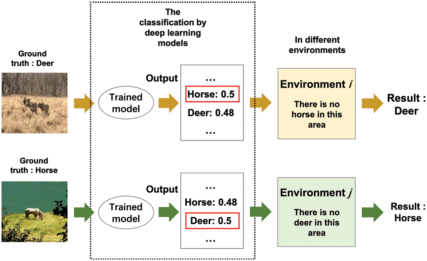
Figure 1: How the distribution of labels increases the accuracy in the environments
In this paper, we built a system EA-DLC (Environment Adaptive Deep Learning based Classification) to improve the accuracy of classification. Our contribution can be summarized as the following. 1) Our system efficiently utilizes the distribution of labels to increase the accuracy with lower cost. The validation set of each environment is labeled by predicted results, which cost is lower than the manual labeling. 2) Our system increases the adaptability of deep learning models in a new environment. Our system only needs to update the distribution of labels in corresponding environment, which is easier than the re-training or transferring of models. We performed our system and existing methods on the samples of CIFAR-10 [12–14], CIFAR-100 [15–17] and Mini-ImageNet [18–20]. All of these evaluations proved the effectiveness of our system.
We organize the paper by the following parts. Section 1 introduces the background and our contributions. Section 2 introduces the existing methods and their problems. In Section 3, we present our system and related analyses. The experiment is organized in Section 4. Section 5 gives the conclusion and future work.
There are many kinds of deep learning models and we selected some of them as the presentative based on the computational resource and the easiness of implementation. VoVNet-57 (Variety of View Network) is designed for object classification task, which consists of blocks including 3 convolution layers and 4 stages modules and outputs stride 32 [21]. The sample is passed through convolutional layers, where here the filters consists of a small receptive field. ResNeSt (Residual networks) is a state-of-art deep learning model for image classification that uses a modular structure with split-attention block and applies attention mechanism to feature-map groups [22]. From ResNeSt50 to ResNeSt269, the structure becomes bigger and more complicated, so that these can get higher accuracy especially when there are more and bigger size training samples. Based on the size of testing samples and computational resource, we use ResNeSt101 in this paper. RepVGG (Re-parameterization Visual Geometry Group) is a classification model, which is improved on the basis of the existing models [23]. DenseNet (Densely Connected Convolutional Network) is a convolutional neural network with dense connections [24]. In this network, there is a direct connection between any two layers, which means the input of each layer connects to all the previous layers. VGG16 is a variant of VGG (Visual Geometry Group) models for image classification [25]. ResNet (Residual Neural Network) allows the original input information to be detoured directly to the output, which simplifies the process and reduces the difficulty of training [26].
These models have been widely used in many applications. Generally, to increase the accuracy of these models, the number of training samples should become bigger while it is a challenge in many applications. Furthermore, the structure of these models becomes bigger that requires some special tuning techniques.
Some fusion operators have applied to improve the performance of classification, which applies multiple models [27]. In that paper, weighted voting method achieved the highest accuracy among all of the other ones. Weighted voting also utilized to construct a more reliable classification system [28]. A sliding window is applied to the weighted majority voting algorithm in that paper. This method applied to a DNN (deep neural network), a CNN (convolutional neural network), and a LSTM (long short-term memory) network to improve the performance [29]. These operators can combine the results of models to improve the accuracy. As the weights play important role to the combination, there should be a validation set to compute these weights. Furthermore, more various models can benefit the improvement of the accuracy. In this paper, we also apply these fusion operators to our system for higher accuracy with some optimizations.
Fig. 2 introduces our system, which is named as EA-DLC (Environment Adaptive Deep Learning based Classification). Firstly, our system trains deep learning models on the training set. Then we run the trained models on a testing sample to get the corresponding outputs that are called as the probabilities of labels. Secondly, we build a validation set that includes some samples of all labels. These samples are labelled by the ground truths, which is called as one-shot guidance. Then we compute the accuracy of each model on these samples. Thirdly, in a new environment, our system builds the validation set and labels this by using the outputs of models, which is called as none guidance (does not need the ground truths). Finally, we apply selective cooperation between the distribution and the probability of labels to get the final result.
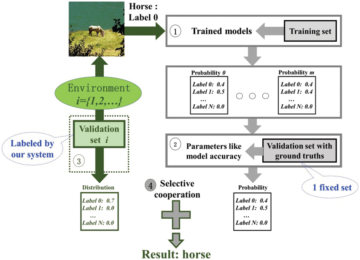
Figure 2: Our system
Firstly, we give some definitions for better explanation. We set
3.1 The Probability of Labels by Trained Model
We define
where here i is the index of the models, n is the index of the samples and k is the index of the labels. When we reconsider the result, we can use
3.2 One-shot Guidance: Validation Set with the Ground Truths
To use the fusion operators, we should build a validation set that is labeled by the ground truths. Then we can use the existing methods that combine the outputs of models as the following:
where here i is the index of the models, n is the index of the samples and k is the index of the labels. In this equation,
3.3 None Guidance: Validation Set Without the Ground Truths
To reduce the dependency of ground truths, our system labels the validation set by using predicted results. In the generally case, the labeling by the predicted results is imprecise. We define the distribution of labels that is computed by the predicted results as below:
where here k is the index of the labels. In this equation,
Generally, the distribution becomes more precise when there are more samples in the validation set. Thus, we should check whether the number of samples is big enough by the following equation
where here k is the index of the labels.
In this subsection, we carried out a selective cooperation between the distribution of labels and the probability of labels. We do not apply the distribution of labels to all results. In more details, when the final result has low probability, it means that the correct result may be the other one. We built selection rules as below:
where here i is the index of the models, n is the index of the samples, k is the index of the labels and x is the index of the predicted label. In this equation,
where here i is the index of the models, n is the index of the samples, k is the index of the labels and x is the index of the predicted label. In this equation,
where here i is the index of the models, n is the index of the samples, k is the index of the labels and x is the index of the predicted label. Compared with EA-DLC-weight, this method does not need the parameter
When a trained model predicts wrong result, we can assume the following relation:
where here i is the index of the models, n is the index of the samples and k is the index of the labels. Then, when we have
In our system, we use the posterior distribution of labels. Thus, as we have introduced in Eq. (3), there is error between the predicted one a real one as bellow:
where here k and q is the index of the labels. When we increase the accuracy of classification, we can have
We evaluated our system and the existing methods on some real datasets. Firstly, we selected and trained the existing deep learning models on the training samples to generate trained models. We trained all of the deep learning models by default settings (we do not change the structure or tune the hyper-parameters many times). We set the number of epochs [34,35] as 10 when training these models. Secondly, we select the testing samples from dataset based on the example distributions, which are to simulate the real distributions in an environment. Then we evaluate our system and the existing methods on the testing samples. When there are random parameters, we evaluate 1000 times and compute the average. At each evaluation step, we randomly select a validation of one-shot guidance (introduced in the Subsection 3.2) and randomly select the validation-sets of none guidance (the range of number is from 1 to 20, which is introduced in the Subsection 3.3). In other words, these validation sets are different to each other, which is to prove the robustness of our system.
4.1 The Evaluation on CIFAR-10
CIFAR-10 has 60000 samples that belong to 10 labels [12–14]. We separated this dataset to 50000 training samples and 10000 testing samples. We use training samples to train the models. We select the samples from the testing set based on different example distributions, which are to simulate the real distributions in the environments.
In the Tab. 1, Zero20 means 20% of the labels have zero samples. We define Zero40 (40% of the labels have zero samples) and Zero80 (80% of the labels have zero samples) by the same way. The labels to be assigned zero samples are randomly selected. Fig. 3 shows the examples of these distributions where the number of samples for the testing set is less than 10000. For example, there are about 6000 testing samples left in Zero40 case. We randomly select 1000 validation samples to compute the distribution of labels. Then, the remained testing samples are used to evaluate the methods. Tab. 1 introduces the accuracies of the methods on the different distributions of the dataset CIFAR-10. As we can see in Tab. 1, our system can increase the accuracy about 0.74% as least and 8.43% as most compared with the existing methods. These results prove the efficiency of our methods.
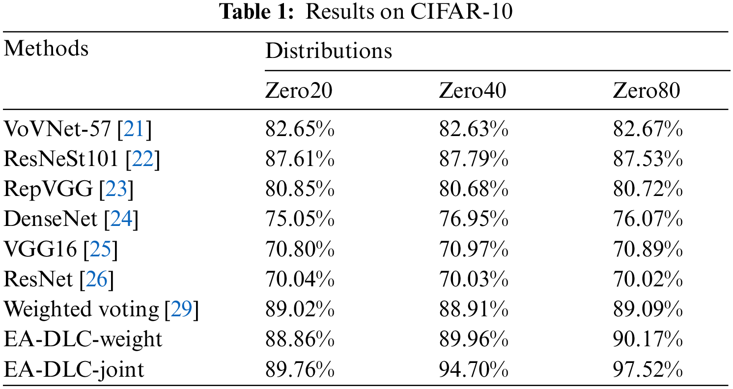
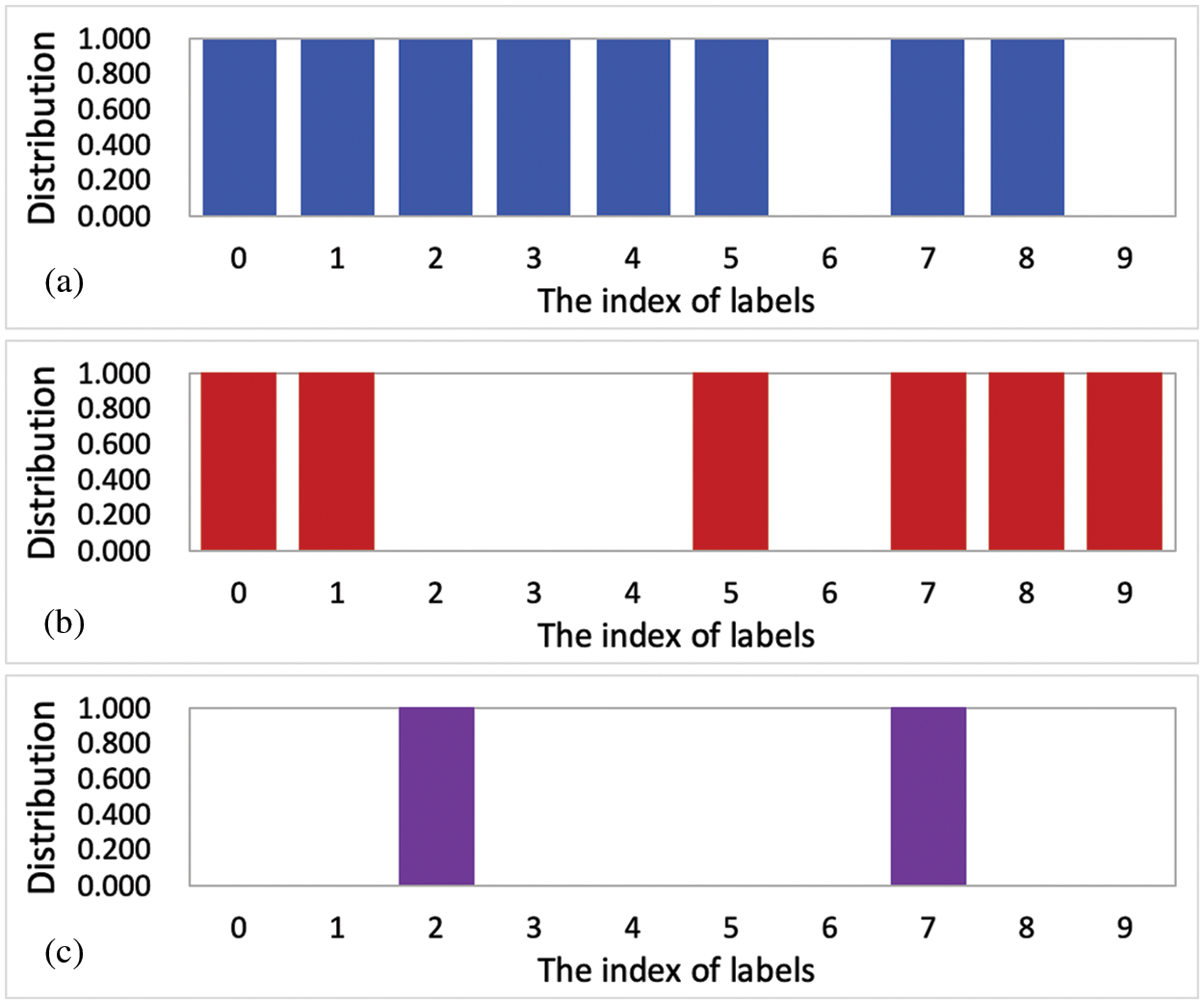
Figure 3: The examples of Zero20, Zero40 and Zero80 on CIFAR-10
4.2 Random Case on CIFAR-100 and Mini-ImageNet
CIFAR-100 has 100 classes and each class contains 600 images [15–17]. We separate each class of the dataset to 500 training samples and 100 testing ones. We use 50000 training samples to train the models. We select the testing samples from these 10000 samples based on different example distributions, which is to simulate the real distributions in the environments.
The Mini-ImageNet dataset is for few-shot deep learning evaluations [18–20]. Its complexity is high as the ImageNet dataset but requires fewer resources compared with the full ImageNet dataset. In total, there are 100 classes and each one has 600 samples of 84 × 84 color images. We use 48000 training samples to train the models. Then we select the samples from the 12000 testing samples based on different example distributions, which is to simulate the real distributions in the environments.
In this subsection, we randomly assign the example distributions to the testing samples. In more details, we randomly select the labels and assign random distributions to the testing set. Fig. 4 shows the examples of random distribution. In this figure,
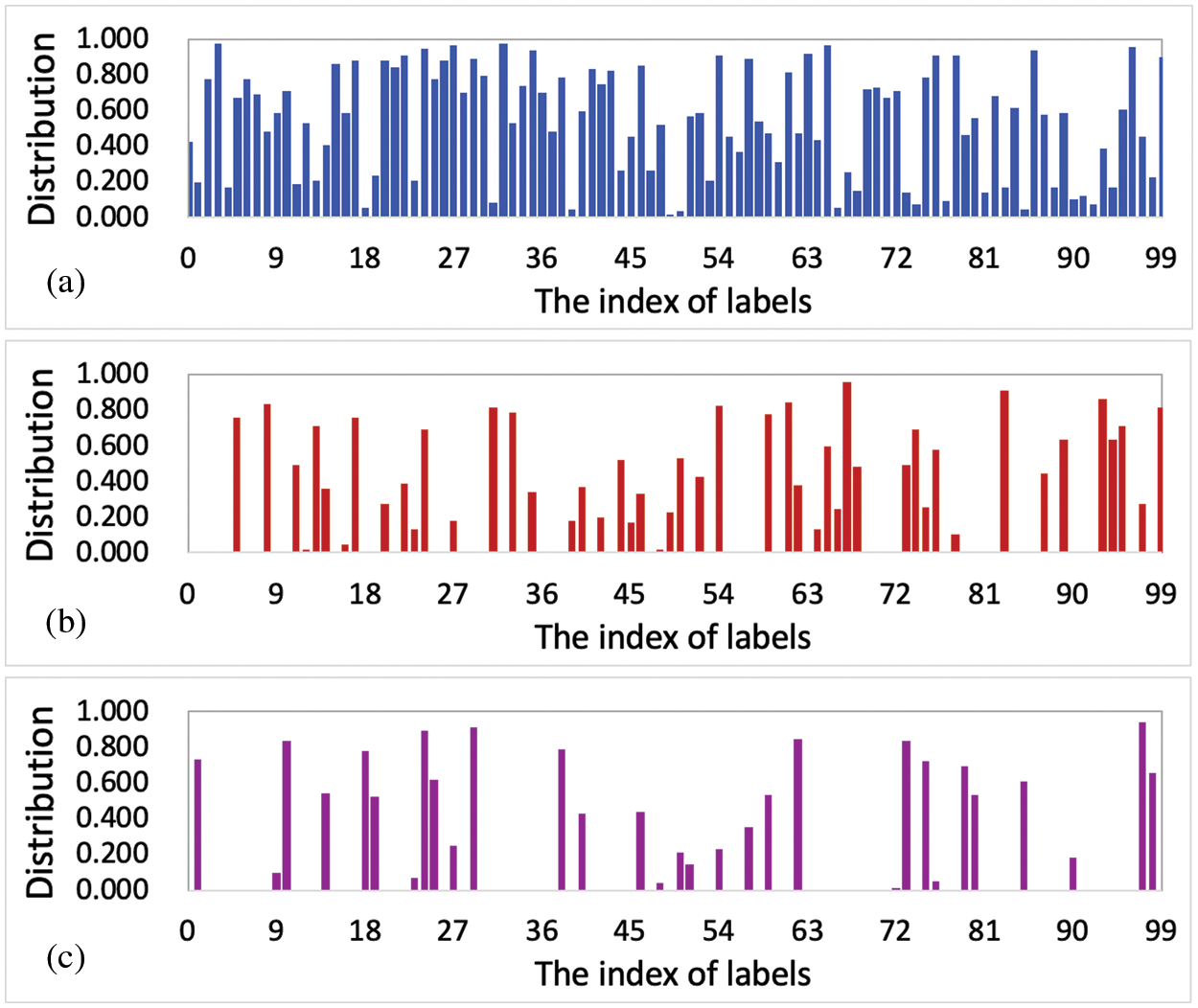
Figure 4: The example distributions. (a)
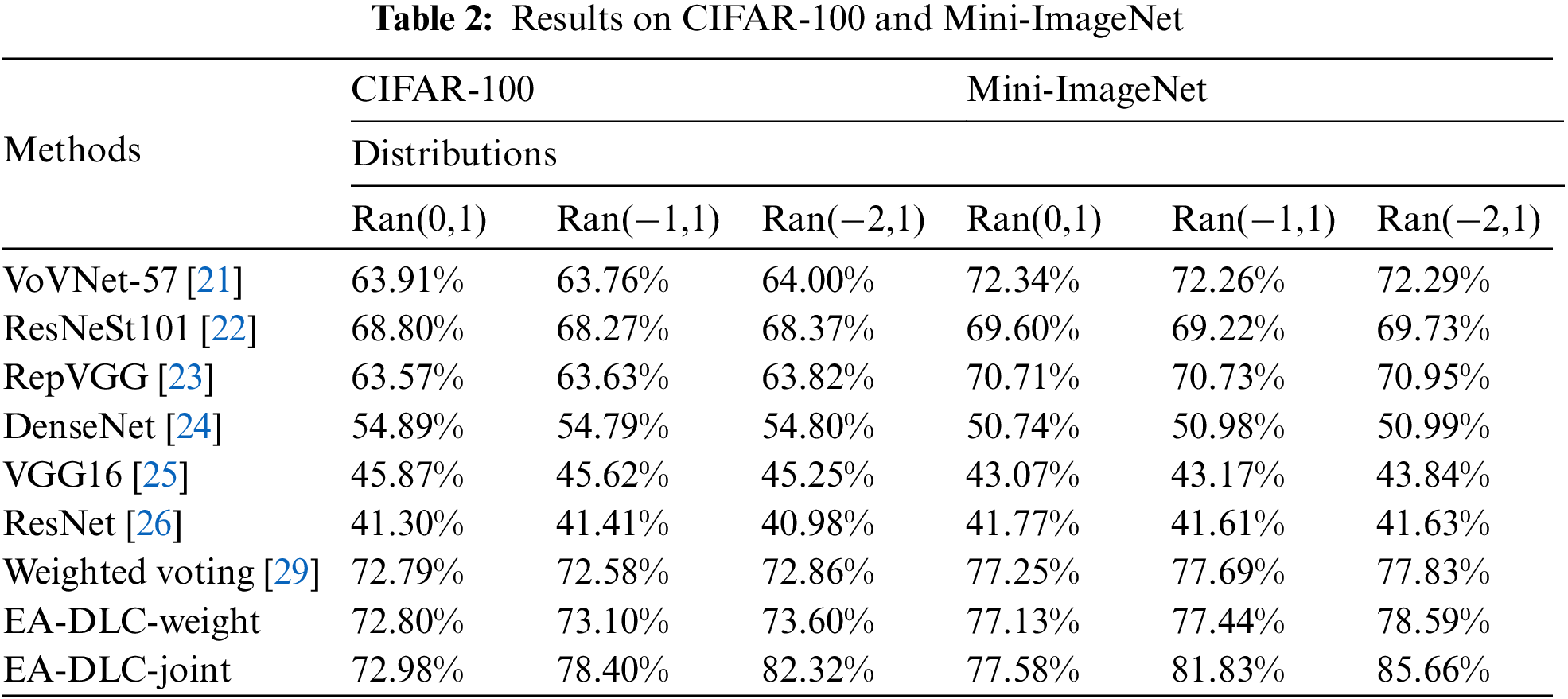
We randomly select 1000 validation samples from the testing set. Then, the remained testing samples are used to evaluate the methods. Tab. 2 introduces the accuracies of the methods on the random distributions of the dataset CIFAR-100 and Mini-ImageNet. As we can see in Tab. 2, our methods can increase the average accuracy about 0.26% (in
Generally, the labels have the balanced number of training samples. Furthermore, the deep structure and multiple layers try to capture the balanced number of features that can classify each label from the others. All these efforts make the trained model achieve similar accuracy on the different distributions.
4.3 The Number of Validation Samples
In this subsection, we evaluated the number of validation samples, which is related to the accuracy. We select the deep learning model VoVNet-57 as a representative to evaluate the parameter. The number of validation samples is important to compute the posterior distribution of labels, which is also related to the accuracy.
Fig. 5 shows that our methods achieved higher accuracy than the existing ones when the number becomes bigger (> 200). The accuracy in increased as the number of samples becomes bigger. This shows that the effect of the error of posterior distribution can be reduced when the number of validation samples is increased.
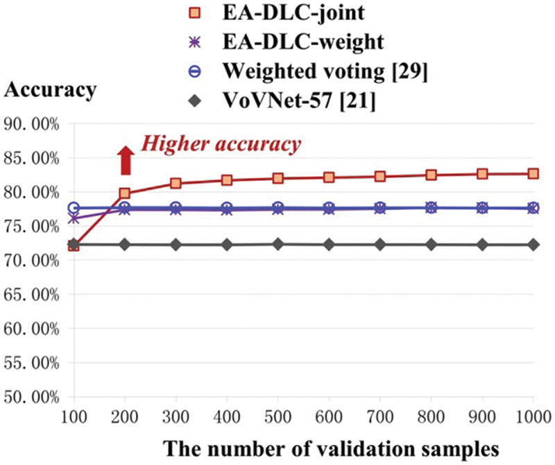
Figure 5: The evaluation on the number of validation samples
We have evaluated our methods and the existing ones on real datasets by applying different distributions. The selected deep learning models performed different accuracies from low (<50%) to high (>87%). Thus, these models can present the general cases when using deep learning models. The results show the effectiveness of our system in these cases. We also evaluated our system in different kinds of simulated environments, which proved the better robustness than the other ones.
Training the models on more labels benefits the range of classification while increasing the difficulty of achieving high accuracy. Transferring or retraining the trained models to the other environments may achieve high accuracy while increasing the cost. Thus, using the distribution of labels in a new environment is a good choice. On the other side, the manual labeling of validation sets is not efficient. Our system solved this problem by labeling the validation set based on the outputs of models. When there are no validation samples, we can temporarily use the existing methods and then collect and label the validation samples. When there are enough (for example, >200 in the Subsection 4.3 case) validation samples of an environment, we can use our system for higher accuracy.
Compared with the fusion operators, our methods can achieve higher accuracy and remain the same cost as all of these only need one validation set. Compared with the single model methods, our methods can achieve higher accuracy than the single model methods. As we applied multiple models, the execution time may be increased, which is related to the number of models. This problem can be solved by executing these models at the same time by using parallel technology [36].
In this paper, we have introduced a novel system that is to increase the accuracy of deep learning model-based classification task. Our system can work well in different environments while reducing the cost of manual labeling. Furthermore, our system can benefit the robustness of the deep learning classification models in different environments.
In the future work, we will do research about the deep cooperation between the output of models and distribution of labels. For example, we can use other outputs of models, which are before the probability of labels (has not been normalized). This may include more information about the features of samples, which can correctly present what the trained model has seen from the samples.
Funding Statement: National Natural Science Foundation of China (Grant Nos. 61802279, 6180021345, 61702281, and 61702366), Natural Science Foundation of Tianjin (Grant Nos. 18JCQNJC70300, 19JCTPJC49200, 19PTZWHZ00020, and 19JCYBJC15800), Fundamental Research Funds for the Tianjin Universities (Grant No. 2019KJ019), and the Tianjin Science and Technology Program (Grant No. 19PTZWHZ00020) and in part by the State Key Laboratory of ASIC and System (Grant No. 2021KF014) and Tianjin Educational Commission Scientific Research Program Project (Grant Nos. 2020KJ112 and 2018KJ215).
Conflicts of Interest: The authors declare that they have no conflicts of interest to report regarding the present study.
References
1. B. Almaslukh, “Deep learning and entity embedding-based intrusion detection model for wireless sensor networks,” Computers, Materials & Continua, vol. 69, no. 1, pp. 1343–1360, 2021. [Google Scholar]
2. S. Kim and S. Lee, “Deep learning approach for cosmetic product detection and classification,” Computers, Materials & Continua, vol. 69, no. 1, pp. 713–725, 2021. [Google Scholar]
3. T. Vaiyapuri, “Deep learning enabled autoencoder architecture for collaborative filtering recommendation in iot environment,” Computers, Materials & Continua, vol. 68, no. 1, pp. 487–503, 2021. [Google Scholar]
4. A. T. Mohamed and S. Santhoshkumar, “Deep learning based process analytics model for predicting type 2 diabetes mellitus,” Computer Systems Science and Engineering, vol. 40, no. 1, pp. 191–205, 2022. [Google Scholar]
5. A. Jayamathi and T. Jayasankar, “Deep learning based stacked sparse autoencoder for papr reduction in ofdm systems,” Intelligent Automation & Soft Computing, vol. 31, no. 1, pp. 311–324, 2022. [Google Scholar]
6. H. Hou, Q. Xu, C. Lan, W. Lu and J. Qin, “UAV pose estimation in GNSS-denied environment assisted by satellite imagery deep learning features,” IEEE Access, vol. 9, no. 1, pp. 6358–6367, 2020. [Google Scholar]
7. H. A., A. H. Alharbi and N. S. Alghamdi, “Breast cancer detection through feature clustering and deep learning,” Intelligent Automation & Soft Computing, vol. 31, no. 2, pp. 1273–1286, 2022. [Google Scholar]
8. R. Wazirali and R. Ahmed, “Hybrid feature extractions and cnn for enhanced periocular identification during covid-19,” Computer Systems Science and Engineering, vol. 41, no. 1, pp. 305–320, 2022. [Google Scholar]
9. W. Min, M. H. Frankosky, B. W. Mott, J. P. Rowe and J. Lester, “DeepStealth: Leveraging deep learning models for stealth assessment in game-based learning environments,” in Int. Conf. on Artificial Intelligence in Education Springer, Madrid, Spain, vol. 9912, no. 1, pp. 277–286, 2015. [Google Scholar]
10. C. Ding, Y. Li, L. Zhang, J. Zhang, L. Yang et al., “Fast-convergent fully connected deep learning model using constrained nodes input,” Neural Processing Letters, vol. 49, no. 3, pp. 995–1005, 2019. [Google Scholar]
11. K. Sharma, A. Alsadoon, P. Prasad, T. Al-Dala’In and D. Pham, “A novel solution of using deep learning for left ventricle detection: Enhanced feature extraction,” Computer Methods and Programs in Biomedicine, vol. 197, no. 1, pp. 1–12, 2020. [Google Scholar]
12. R. D. Gottapu and C. H. Dagli, “Efficient architecture search for deep neural networks,” Procedia Computer Science, vol. 168, no. 1, pp. 19–25, 2020. [Google Scholar]
13. H. Zhang and M. Xu, “Improving the generalization performance of deep networks by dual pattern learning with adversarial adaptation,” Knowledge-Based Systems, vol. 200, no. 1, pp. 1–10, 2020. [Google Scholar]
14. X. Li, M. Xu, J. Xu, T. Weise and Z. Wu, “Image retrieval using a deep attention-based hash,” IEEE Access, vol. 8, no. 1, pp. 142229–142242, 2020. [Google Scholar]
15. M. Y. Huang, C. H. Lai and S. H. Chen, “Fast and accurate image recognition using deeply-fused branchy networks,” in 2017 IEEE Int. Conf. on Image Processing (ICIP) IEEE, Beijing China, vol. 2017, no. 1, pp. 2876–2880, 2018. [Google Scholar]
16. B. Stuhr and J. Brauer, “CSNNS: Unsupervised, backpropagation-free convolutional neural networks for representation learning,” in 2019 18th IEEE Int. Conf. on Machine Learning and Applications (ICMLA) IEEE, Boca Raton, Florida, USA, vol. 1, no. 1, pp. 1613–1620, 2020. [Google Scholar]
17. C. Termritthikun, Y. Jamtsho and P. Muneesawang, “An improved residual network model for image recognition using a combination of snapshot ensembles and the cutout technique,” Multimedia Tools and Applications, vol. 79, no. 1, pp. 1475–1495, 2020. [Google Scholar]
18. Y. Zhang, M. Fang and N. Wang, “Channel-spatial attention network for fewshot classification,” PLoS ONE, vol. 14, no. 12, pp. 1–16, 2019. [Google Scholar]
19. W. Bing, B. Kha, G. Lei, B. Xsta and B. Yza, “A biologically inspired visual integrated model for image classification,” Neurocomputing, vol. 405, no. 1, pp. 103–113, 2020. [Google Scholar]
20. H. J. Ye, H. Hu and D. C. Zhan, “Learning adaptive classifiers synthesis for generalized few-shot learning,” International Journal of Computer Vision, vol. 129, no. 6, pp. 1930–1953, 2021. [Google Scholar]
21. Y. Lee, J. W. Hwang, S. Lee, Y. Bae and J. Park, “An energy and GPU-computation efficient backbone network for real-time object detection,” in 2019 IEEE/CVF Conf. on Computer Vision and Pattern Recognition Workshops (CVPRW) IEEE, Long Beach, CA, USA, vol. 2019, no. 1, pp. 752–760, 2019. [Google Scholar]
22. S. Wang, Y. Liu, Y. Qing, C. Wang and R. Yao, “Detection of insulator defects with improved ResNeSt and region proposal network,” IEEE Access, vol. 8, no. 1, pp. 184841–184850, 2020. [Google Scholar]
23. X. Feng, X. Gao and L. Luo, “X-SDD: A new benchmark for hot rolled steel strip surface defects detection,” Symmetry, vol. 13, no. 4, pp. 706–721, 2021. [Google Scholar]
24. Z. Zhang, X. Liang, X. Dong, Y. Xie and G. Cao, “A sparse-view CT reconstruction method based on combination of DenseNet and deconvolution,” IEEE Transactions on Medical Imaging, vol. 37, no. 6, pp. 1407–1417, 2018. [Google Scholar]
25. Z. Liu, J. Wu, L. Fu, Y. Majeed and Y. Cui, “Improved kiwifruit detection using pre-trained VGG16 with RGB and NIR information fusion,” IEEE Access, vol. 8, no. 1, pp. 2327–2336, 2020. [Google Scholar]
26. S. Zhao, L. Qiu, P. Qi and Y. Sun, “A novel image classification model jointing attention and ResNet for scratch,” IWCMC, vol. 1, no. 1, pp. 1498–1503, 2020. [Google Scholar]
27. A. Giuseppe, C. Domenico, M. Antonio and P. Antonio, “Multi-classification approaches for classifying mobile app traffic,” Journal of Network and Computer Applications, vol. 103, no. 1, pp. 131–145, 2018. [Google Scholar]
28. Y. You, F. Li and X. Li, “On redundant weighted voting systems with components having stochastic arrangement increasing lifetimes,” Operations Research Letters, vol. 49, no. 5, pp. 777–784, 2021. [Google Scholar]
29. X. Liu and A. G. Richardson, “Edge deep learning for neural implants: A case study of seizure detection and prediction,” Journal of Neural Engineering, vol. 18, no. 4, pp. 1–16, 2021. [Google Scholar]
30. D. Li, M. H. Bawany, A. E. Kuriyan, R. S. Ramchandran and G. Sharma, “A novel deep learning pipeline for retinal vessel detection in fluorescein angiography,” IEEE Transactions on Image Processing, vol. 29, no. 1, pp. 6561–6573, 2020. [Google Scholar]
31. P. M. Maloca, P. Müller, A. Y. Lee, A. Tufail and N. Denk, “Unraveling the deep learning gearbox in optical coherence tomography image segmentation towards explainable artificial intelligence,” Communications Biology, vol. 4, no. 1, pp. 1–12, 2021. [Google Scholar]
32. H. Zhang, Y. Zhang and X. Geng, “Practical age estimation using deep label distribution learning,” Frontiers of Computer Science (Print), vol. 15, no. 3, pp. 1–6, 2021. [Google Scholar]
33. Y. Shi, J. Liu, B. Wang, Z. Qi and Y. J. Tian, “Deep learning from label proportions with labeled samples,” Neural Networks, vol. 128, no. 1, pp. 73–81, 2020. [Google Scholar]
34. A. Urushibara, T. Saida, K. Mori, T. Ishiguro and T. Masumoto, “Diagnosing uterine cervical cancer on a single T2-weighted image: Comparison between deep learning versus radiologists,” European Journal of Radiology, vol. 135, no. 6, pp. 1–16, 2020. [Google Scholar]
35. S. T. Yekeen, A. L. Balogun and K. Yusof, “A novel deep learning instance segmentation model for automated marine oil spill detection,” ISPRS Journal of Photogrammetry and Remote Sensing, vol. 167, no. 1, pp. 190–200, 2020. [Google Scholar]
36. T. T. Leonid and R. Jayaparvathy, “Classification of elephant sounds using parallel convolutional neural network,” Intelligent Automation & Soft Computing, vol. 32, no. 3, pp. 1415–1426, 2022. [Google Scholar]
 | This work is licensed under a Creative Commons Attribution 4.0 International License, which permits unrestricted use, distribution, and reproduction in any medium, provided the original work is properly cited. |