Computers, Materials & Continua DOI:10.32604/cmc.2022.027443
Article

Real-Time Demand Response Management for Controlling Load Using Deep Reinforcement Learning

Yongjiang Zhao, Jae Hung Yoo and Chang Gyoon Lim*

Department of Computer Engineering, Chonnam National University, Yeosu, 59626, Korea
*Corresponding Author: Chang Gyoon Lim. Email: cglim@jnu.ac.kr
Received: 18 January 2022; Accepted: 12 April 2022

Abstract: With the rapid economic growth and improved living standards, electricity has become an indispensable energy source in our lives. Therefore, the stability of the grid power supply and the conservation of electricity is critical. The following are some of the problems facing now: 1) During the peak power consumption period, it will pose a threat to the power grid. Enhancing and improving the power distribution infrastructure requires high maintenance costs. 2) The user's electricity schedule is unreasonable due to personal behavior, which will cause a waste of electricity. Controlling load as a vital part of incentive demand response (DR) can achieve rapid response and improve demand-side resilience. Maintaining load by manually formulating rules, some devices are selective to be adjusted during peak power consumption. However, it is challenging to optimize methods based on manual rules. This paper uses Soft Actor-Critic (SAC) as a control algorithm to optimize the control strategy. The results show that through the coordination of the SAC to control load in CityLearn, realizes the goal of reducing both the peak load demand and the operation costs on the premise of regulating voltage to the safe limit.

Keywords: Demand response; controlling load; SAC; CityLearn

1  Introduction

Global buildings consumed 30% of total energy and generated 28% of total carbon emissions in 2018, which leads to economic and environmental concerns. Therefore, it is of great significance to reduce energy consumption, energy cost, and carbon emission of buildings while maintaining user comfort. Demand-side management (DSM) is the effective strategy to solve this problem, and it's one of the important functions in a smart grid that allows customers to make informed decisions regarding their energy consumption and helps the energy providers reduce the peak load demand and reshape the load profile [1]. As a typical way of DSM, demand response is considered the most cost-effective and reliable solution for smoothing the demand curve when the system is under stress [2].

Various DR programs have been developed and implemented. It is mainly divided into price-based and incentive-based methods. The price-based method is mainly based on changing the electricity price to affect the way users use electricity. The difference is that the incentive-based process changes the way users use electricity by giving them economic incentives. Controlling load as an essential part of incentive DR can control the user's load during the peak period of power consumption, avoid the threat to the grid during the peak period of power consumption, save the user's electricity expenditure, and reasonably arrange the power usage plan. This paper is mainly aimed at finding some feasible control algorithms based on incentives. While reducing the operating cost of the power supply company improves the efficiency of users’ electricity consumption. This process ensures the stability and risk avoidance of the power grid during the peak period of power consumption.

There are many traditional control methods based on rule feedback, which are mainly divided into two types: (1) relying on pre-set values for control (such as temperature adjustment of air conditioners), and (2) performing proportional-integral-derivative (PID) control based on previous historical data points. The control strategy based on rule feedback is efficient and straightforward, but it is not optimal for two reasons. First, the predicted information is not considered. For example, the room temperature may become hot in the future, but it will not cool down in advance. Second, like the PID algorithm, some parameters need to be set before use. It cannot be automatically adjusted under the particular building and climatic conditions. The model predictive control (MPC) has been explored to improve performance.

Machine learning (ML) has been used in almost every stage of the building lifecycle and has demonstrated its potential to enhance building performance. As a branch of machine learning specifically for control problems, reinforcement learning (RL) is becoming a promising method to revolutionize building controls [3]. Traditional RL (such as Q-Learning) can only complete simple tasks (limited environment and limited actions), and it is very difficult to complete complex tasks. Unlike traditional model-based methods that require an explicit physical or mathematical model of the system, deep reinforcement learning (DRL), a combination of reinforcement learning and deep learning [4], is a better solution to solve complex control problems [5].

DRL has developed rapidly in recent years, and many solutions have been proposed. Such as trust region policy optimization (TRPO) on-policy algorithm [6], proximal policy optimization (PPO) on-policy algorithm [7], asynchronous advantage actor-critic (A3C) on-policy algorithm [8], deep deterministic policy gradient (DDPG) off-policy algorithm [9] and twin delayed DDPG (TD3) off-policy algorithm [10], etc. However, these methods typically suffer from two significant challenges: very high sample complexity and brittle convergence properties, which necessitate meticulous hyper-parameter tuning. Both challenges severely limit the applicability of such methods to complex, real-world domains [11]. The SAC algorithm was proposed in 2018 by Tuomas Haarnoja, and the performance was further improved [12]. It can solve the above two problems well and can complete the tasks in the real world. Therefore, this paper uses the SAC as the control algorithm to reduce the peak voltage by controlling the user's load (such as heat pump and electric heater) or increase power consumption during the valley period of power consumption for daily energy storage. It can maintain a stable power supply to the grid and maximize the profit of the power supply company in CityLearn [13]. At the same time, rationally adjust users’ electricity consumption and reduce carbon dioxide emissions.

The remaining of the paper is organized as follows. Section 2 introduces the background and scenarios in which the DRL and CityLearn are presented, respectively. Section 3 is the methodology that uses the SAC to optimal DR strategy for controlling load. Section 4 Use the Hot-Humid climate zone as a case study and use the SAC to learn and optimize control strategies, then display and analyzes the results. At last, the conclusions are drawn in Section 5.

2  Review of Related Works

Reference [14] reviews the use of RL for DR applications in the smart grid from 1997 to 2018. Energy systems that use reinforcement learning as a control strategy are mainly heating, ventilation, and air conditioning (HVAC) system [15], domestic hot water (DHW), and electric vehicle (EV) systems [16], battery and photovoltaics (PV) system [17], hybrid electric vehicle (HEV) system [18], DHW [19], thermal storage [20], and heat pump [21]. The main control strategy algorithms used by these systems are Q-Learning, Actor-Critic, and batch reinforcement learning (BRL). Q-Learning can only be used in discrete action spaces, while most energy control systems are in continuous action spaces. The Q-Learning strategy is relatively easy, requires a Q table, and uses relatively tiny data, especially experience replay. However, suppose the action space is a discrete and high-dimensional value. In that case, the resulting strategy is uncertain, and convergence cannot be guaranteed when the neural network is used for fitting. BRL is a learning method that uses data composed of fixed and pre-collected transition experiences for optimal strategy learning. RL Agent does not interact with the environment and only learns from offline samples with a fixed amount of data. BRL learning is very slow in practical applications, and there are problems such as low efficiency caused by random approximation. At present, experience replay and double deep Q-Network (DDQN) provide corresponding solutions. Actor-Critic adds a critical part based on policy gradient and can be updated in a single step faster than the traditional policy gradient. But Actor-Critic depends on the Critic's value judgment. It is difficult for critics to converge, and coupled with actor updates, it is even more difficult to converge. Google DeepMind proposed an improved Actor-Critic algorithm DDPG, which combines the advantages of deep Q-Network (DQN). The problem of difficulty in convergence is solved.

More and more deep reinforcement learning algorithms have been proposed and applied to the DR management control problem combined with deep learning. Such as DQN, DDPG, DDQN, TRPO, PPO, etc. [22] proposed the use of DDPG in smart homes to optimize the power consumption strategy of PV, energy storage system (ESS), HVAC. [23] is proposed to adjust the energy consumption of PV, ESS, and EV through PPO in residential buildings. [24] and [25] used DDQN and TRPO, respectively, in the control optimization problem in the smart home. This application provides users with a comfortable environment while reducing energy consumption. Two main challenges of model-free RL are poor sample efficiency and brittle convergence properties. On-policy algorithms like PPO, TRPO require new samples to be collected for each extravagantly expensive gradient step. Off-policy algorithms, like DDPG, DDQN provide for sample-efficient learning but are notoriously challenging to use due to their extreme brittleness and hyperparameter sensitivity.

The poor sample efficiency and brittle convergence properties are two major difficulties that prevent PPO, TRPO, DDPG, and DDQN from being more widely used in energy management systems. In order to meet the above two challenges, this paper uses the SAC as the main algorithm to optimize the optimization strategy of the energy management system. The SAC is an off-policy algorithm, and it can save the previous learning experience in a buffer and reuse it to solve the problem of poor sample efficiency. In terms of control strategy, the SAC uses a random action strategy and maximizes the entropy of the strategy while maximizing rewards. Maximizing the entropy of the strategy can make the actions as random as possible while reaching the goal. The advantage of this is to better explore the environment, avoid converging to the local optimum, and make the training more stable. The SAC has fewer hyper-parameters, is not very sensitive to parameters, and can adapt to different complex environments. The SAC algorithm showed substantial improvement in both performance and sample efficiency over both off-policy and on-policy prior methods. This current research investigates the suitability of the SAC algorithm for tackling the district DSM problem utilizing CityLearn [25]. CityLearn is an open-source framework implemented using OpenAI Gym standard that can use reinforcement learning algorithm simulation for energy management, demand response management, and load-shaping. CityLearn provides electricity demand data in 4 different climate zones, each with nine buildings. The energy demand for each building has been pre-simulated using EnergyPlus in a different climatic zone of the USA (2A | Hot-Humid | New Orleans; 3A | Warm-Humid | Atlanta; 4A | Mixed-Humid | Nashville; 5A | Cold-Humid | Chicago) [25]. The types of buildings are office, restaurant, retail and multi-family buildings.

3  Methodology

3.1 DR Management for Controlling Load Architecture

There are many buildings in a climate zone, and each building is equipped with a water storage tank, heat pump, electric heater, PV array, and battery, as shown in Fig. 1. These devices can be used selectively in CityLearn. The heat pump can provide hot and cold water. In CityLearn, the heat pump is mainly used for cooling, and the electric heater is used for heating. The temperature setpoints for heat pump cooling and electric heater heating are constant (do not need to be adjusted frequently in daily life). The cooling temperature is 7°C–10°C, and the heating temperature is 50°C.

Figure 1: DR management for controlling load workflow

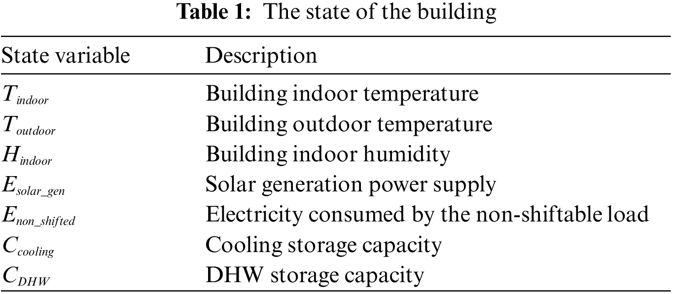
The Agent is a controller, which can control the charging and release of the water storage tank. The control strategy can be learned using a deep neural network. The State is the energy demand and power consumption of the building, as shown in Tab. 1. The Action is the operation of the controller on the water storage tank (described in detail below). The controllable loads are a heat pump and an electric heater. The Agent does not directly control them but indirectly controls the power consumption of the heat pump and electric heater by controlling the charging and releasing of the water storage tank, cause the temperature of the heating storage tank and cooling storage tank should be maintained at 50°C and 7°C–10°C, respectively. The task of the whole system is to optimize the control strategy of the controllable equipment through the Agent, to reduce the power consumption of the controllable load on the premise of meeting the energy demand.

In Citylearn, the storage capacity of cooling energy storage and DHW energy storage at time t is recorded as Ct.

Ct+1=Ct+max{min{at⋅Cmax,Cmax},−Cdem}(1)

Ct: The capacity of the storage device at time t, [Cdem,Cmax].

Cmax: The maximum storage capacity of the storage device, [0,+∞).

at: The control strategy (Action) of the storage device, [−1Cmax,1Cmax].

Cdem: The demand for energy in buildings, [0,+∞).

In Eq. (1), when at is executed, if at>0, it indicates that the storage device needs supplementary energy (cooling or DHW), and the supplementary capacity of the storage device is at⋅Cmax. For example, at<0, it indicates that the storage device needs to release excess energy (release to the building), but the released capacity cannot be less than −Cdem, and it must first meet the daily energy demand of the building.

When the action at>0 is executed, the storage device requires heat pump and electric heater to convert the energy consumed by the heat pump and electric heater into cold energy and heat energy to supplement the required energy.

The electric energy required by the heat pump to produce cold energy is:

Ehp=Ct(cooling)η1(2)

The electric energy required by the electric heater to generate heat is:

Eeh=Ct(DHW)η2(3)

where η1 is the conversion efficiency coefficient of cold energy, the value is [0.2,0.3]. η2 is the coefficient of thermal energy conversion efficiency, with a value of 0.9.

Reward (Rtotal) is defined as follows in CityLearn:

Rtotal=Esolar_gen−(Ehp+Eeh+Enon_shifted)(4)

where Enon_shifted is the electrical energy consumed by non-shifted load. Esolar_gen is the electric energy generated by the solar generation (in most cases, Esolar_gen is less than the sum of the consumed electric energy).

3.2 SAC-Based Real-Time DR Management Architecture

This paper uses the data of the Hot-Humid climate zone. In order to enable the DRL controller to control in real-time, deploying the controller on each building can speed up the response speed of the control. Fig. 2 shows the real-time DR management system workflow. The whole process is divided into input, data preprocessing, data processing unit, and output parts.

Figure 2: The real-time DR management system workflow

The input part is mainly responsible for obtaining environmental data from the building, such as temperature, humidity, power consumption of equipment, and energy storage equipment storage status. These data reflect the State of the building is located and the State of electricity consumption by users. Using this data information, DR control strategies can be optimized through data mining. To avoid redundant data feature input, it is necessary to extract the principal components of the data before data processing. It not only reduces the dimensionality of data input but also improves the robustness of the system. The data processing unit is the system's main component, using principal components analysis (PCA) to realize data processing. The input is the data of the building, called State. The output terminal outputs the action that controls the increase or decrease of DHW, cooling, and battery, called action. The Agent is realized by deep neural network fitting. The training process will be described in detail later, and it can be considered that it has been trained. The output terminal is responsible for the control of the device. Turn off some equipment during the peak power supply period of the power grid to reduce the demand for electricity and increase the stability of the power supply to the power grid. On the contrary, use energy storage equipment for energy storage during low peak periods to increase the equipment's electricity use. Making the user's electricity consumption curve as smooth as possible in a day guarantees user's daily demand for energy and enables users to have a comfortable living environment.

3.3 SAC-Based Algorithm for DR Management

This paper uses the SAC as the control strategy algorithm for real-time DR management of controlling load. The SAC implements the overall architecture diagram of the control strategy system in the CityLearn, as shown in Fig. 3. The system is mainly divided into two parts, one is online, and the other is offline. Offline is the main training part of the SAC, including the Critic and the Actor. Online only contains the Actor responsible for real-time decision-making.

Figure 3: The SAC operation framework

In offline, the Actor make action through decision function, while critics make predictions based on the Actor's actions. After the Actor gets the critic score, it continuously improves the strategy function to obtain higher scores. When the actor training is completed, share the hyper-parameters of the actor network online. The Actor can make real-time decisions based on the State of the environment.

The specific operation process is shown in Fig. 4. Online needs to obtain data st from the building. The distribution πϕ(st,at) of at concerning st is obtained after the Actor makes the decision. The system randomly samples action at. After at is executed, the Critic scores the action performed by the Actor based on st and at. In offline, actors use critic scores to maximize entropy, thereby ensuring higher scores in the next round of decision-making. When the Actor performs the action, the environment will feedback rewards. The Critic will use its own score to compare with the reward value of environmental feedback. Improve the accuracy of the prediction score by seeking loss. Finally, back-propagation updates the network parameters.

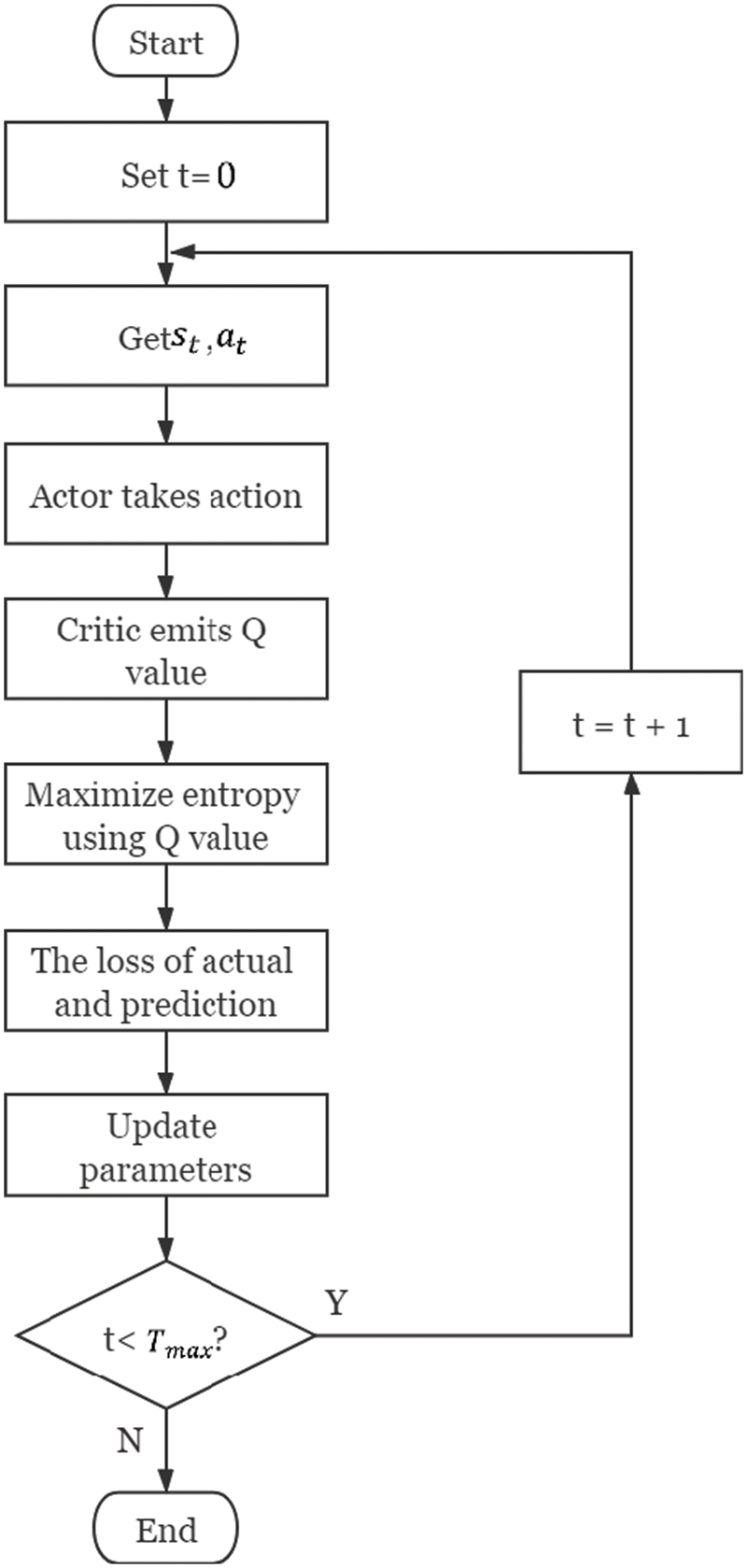
Figure 4: The flow chart of SAC

The goal of the SCA is to maximize the entropy of the strategy while maximizing rewards. The specific method is to add policy entropy H(π(⋅|st)) to the reward item. In this way, the higher the policy entropy, the larger the reward value will be. After adding the policy entropy, the objective function is as follows Eq. (5):

J(π)=∑t=0TE(st,at)∼ρπ[r(st,at)+αH(π(⋅|st))](5)

The temperature coefficient α controls the importance of the strategy entropy relative to the initial reward and also controls the strength of the strategy's randomness. The larger the α, the higher the randomness of the strategy.

In the following derivation, α is omitted because its effect is equivalent to multiplying the initial reward by 1α. The Actor selects the appropriate action based on the State, and The Critic evaluates the value of the State. In order to make the training more stable, Critic uses four functions. Two state value functions are represented by ψ and ψ¯, and two action-state value functions are represented by θ1 and θ2. Among them, the target state value function ψ¯ is not trained, but through the soft update to ψ¯.

ψ¯←τψ+(1−τ)ψ¯(6)

This method is very similar to the DDPG method, and ψ minimizes the squared difference distance of Q function through training. This is very similar to the traditional critic loss function, except that the policy entropy is added.

JV(ψ)=Est∼D[12(Vψ(st)−Eat∼πϕ[Qθ(st,at)−log⁡πϕ(at|st)])2](7)

where D is a replay buffer. Obtain the gradient by derivation:

∇^ψJV(ψ)=∇ψVψ(st)(Vψ(st)−Qθ(st,at)−log⁡πϕ(at|st))(8)

The dynamic action-value functions θ1, θ2 use the same objective function for training. The reason for using two-state actions here is to take the minimum value when updating the Actor later to prevent overestimation of the value. This method is similar to the DDQN method. Loss function is also to minimize the squared difference between the estimated value and the target value, and the formula is shown in Eq. (9).

JQ(θ)=E(st,at)∼D[12(Qθ(st,at)−r(st,at)+γEst+1∼p[Vψ¯(st+1)])2](9)

Obtain the gradient by derivation:

∇^θJQ(θ)=∇θQθ(at,st)(Qθ(st,at)−r(st,at)+γVψ¯(st+1))(10)

The goal of the Actor is to minimize the Kullback-Leibler divergence between the strategy and the exponential function. In other words, the probability of an Actor taking action is directly proportional to the value index of this action. The larger the action value, the greater the probability of taking this action, as shown in the following Eq. (11):

Jπ(ϕ)=Est∼D[DKL(πϕ(⋅|st)||exp⁡(Qθ(st,⋅))Zθ(st))](11)

where Zθ is the distribution function, which does not involve the subsequent derivation process and can be ignored, the derivation of Eq. (11) will encounter problems because the Actor's actions are randomly sampled from a random strategy distribution. The sampling process is not derivable, so a reparameterized trick is needed to solve this problem. Replace the randomness of the sampling with the randomness of the random input noise, as shown in the following Eq. (12).

at=fϕ(εt;st)(12)

where εt is an input noise vector sampled from some fixed distribution, such as a spherical Gaussian. The objective function of the Actor can be written in the following form:

Jπ(ϕ)=Est∼D,εt∼N[log⁡πϕ(fϕ(εt;st)|st)−Qθ(st,fϕ(εt;st))](13)

where πϕ is defined implicitly in terms of fϕ. We can approximate the gradient of Eq. (14) with

∇^θJπ(ϕ)=∇ϕlog⁡πϕ(at|st)+(∇atlog⁡πϕ(at|st)−∇atQ(st,at))∇ϕfϕ(εt;st)(14)

4  Case Study and Result Analysis

4.1 Case Scenario

The CityLearn has a total of 4 climate zones. In the case scenario, the Hot-Humid climate zone is used as a typical case for research. Considering the differences in equipment installed in different buildings, Cooling storage tank is installed in all buildings in Hot-Humid. Except for retail_1 and retail_2, DHW storage tank is installed in other buildings. PV is installed in office, retail_2, multi_family_1 and multi_family_2, but not in other buildings, as shown in Tab. 2. Although the equipment of each building is different, the controllable load is installed, which does not affect its use as a case study in this paper.

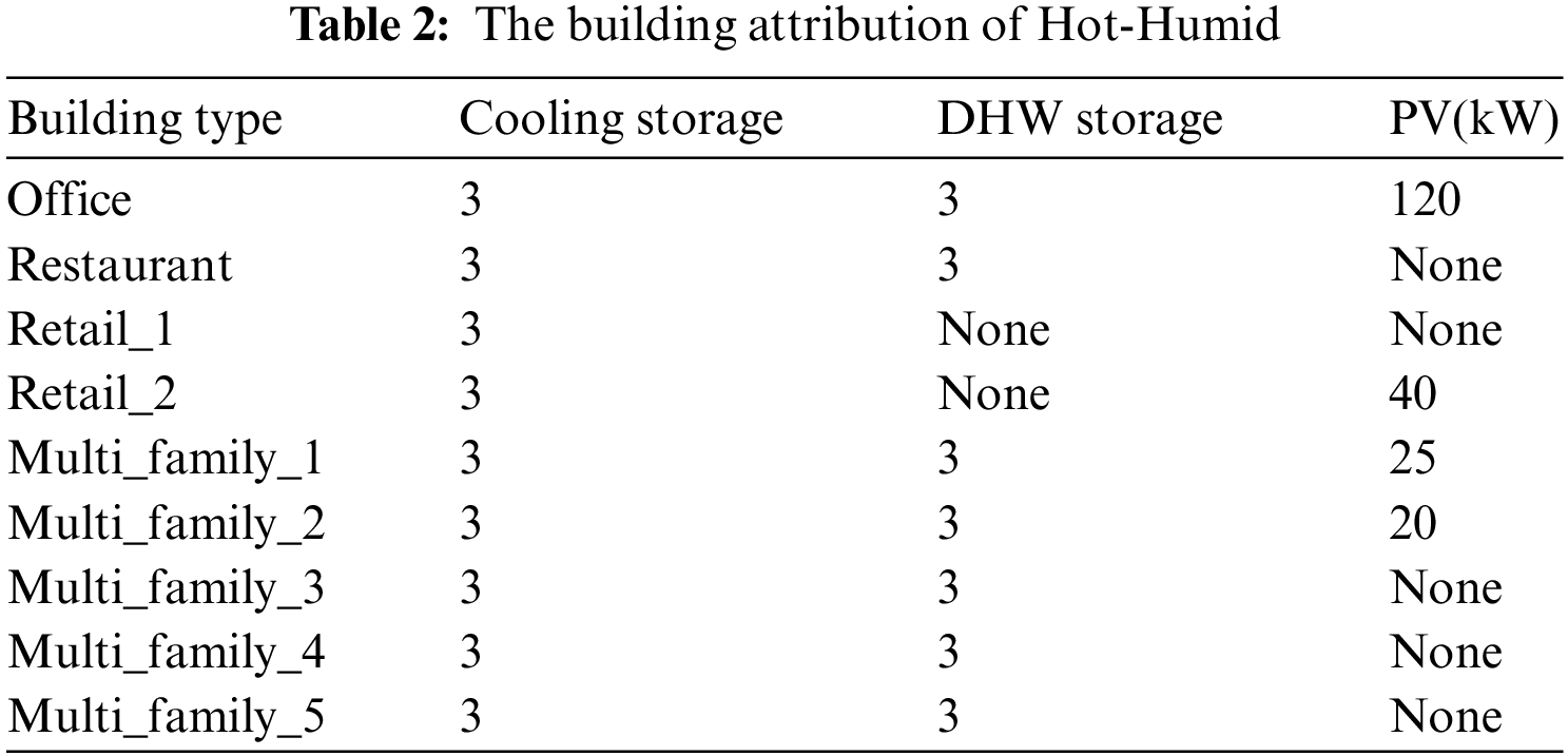
There are measuring devices in each building: electricity meters, the State of a charge measuring device for storage equipment, and temperature and indoor humidity sensors. Measured every hour, 24 data points can be generated in a day. The capacity of a storage device is a multiple of the maximum heating or cooling demand that the storage device can store in a given time. In Hot-Humid, except for retail_1 and retail_2, where the DHW storage device is not installed, the rest are installed. Their capacity is three times the maximum cooling or DHW demand. New Orleans is located in Louisiana. The average commercial price is lower than the average residential price. Therefore, the installation of PV arrays in residences can reduce power consumption.

4.2 Simulation Parameter Setting

According to the above scenario, observation state, control action, and immediate reward are defined in Section 3.1. To improve the response speed of DR management, a decentralized deployment model is adopted in the case scenario. Each building has its own measuring devices, controllers, and actuators, so the number of variables in State, Action, and reward is nine. The exception is that the variable net electricity consumption is the sum of the electricity consumed by nine buildings at a specific time in the State. By observing net electricity consumption, the trained controller can adjust its energy consumption strategy. The capacity in the building where the storage device is installed is 3, and the range of at is [−13,13].

To accelerate the training of the SAC, two Q networks are used during training, namely Q1 and Q2. Their value functions are target Q1 and target Q1, respectively. The minimum value in Q1 and Q1 is taken as the score of a specific action, and the reason is to prevent the Critic from giving too high a score to the Actor, which is not easy to converge. The hyperparameters used in training the network are shown in Tab. 3.

4.3 Results and Analysis

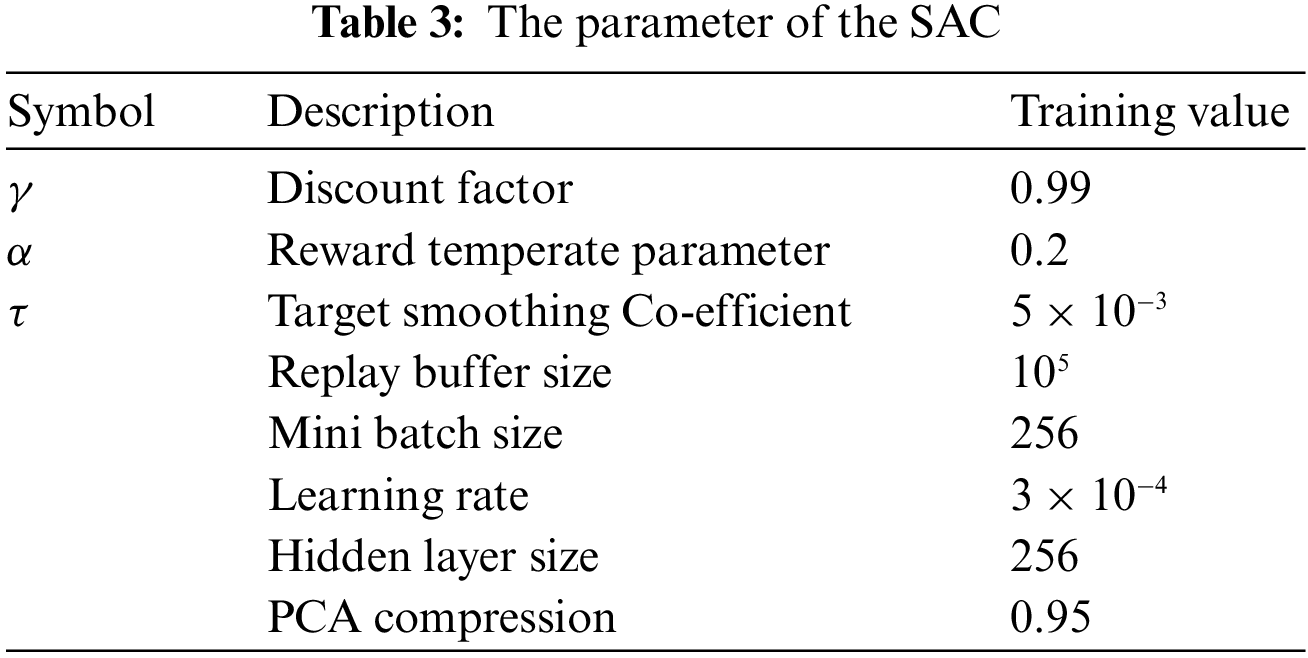
Replay buffer size is the maximum number of Markov Decision Process (MDP) tracks (st,at,rt,st+1) that can be stored, with a capacity of 105. The discount factor is the discount for future rewards, and here it is 0.99. Reward template parameter a determines the relative importance of the entropy term against the reward, thus controlling the optimal policy's stochasticity, which is 0.2. Target smoothing coefficient τ is the weight of updating network parameters from Q to target, 0.005.

The main task of the previous case scenario is to help the controller make decisions through deep reinforcement learning algorithms, thereby optimizing the controller's control strategy. The purpose of the controller is to control the load (cooling and DHW storage device) by observing the data of the building's measuring device, which reduces the total power consumption of the building while maximizing the demands of users for cooling and DHW. To optimize the optimization strategy of the controller, this paper uses the SAC as the Agent to explore and learn in the case scenario. The average reward curve obtained by the SAC learning in each building is shown in Fig. 5.

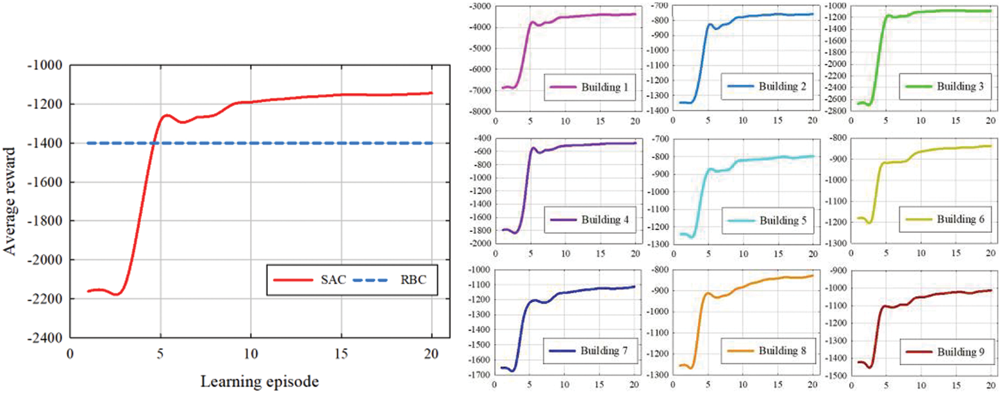
Figure 5: The average reward for all buildings and their respective reward

A rule-based controller (RBC) is a controller that sets rules manually and cannot explore, learn, and optimize its own strategies. The SAC learning curve surpassed the RBC after exploring 5 episodes, indicating that the control algorithm using the SAC as the controller can optimize the control strategy and make better decisions in different scenarios. While reducing building power consumption, it also reduces electricity costs. As episodes continue to increase, the controller gets more and more rewards. It shows that the controller has gradually found a way to optimize the control strategy and made better decisions. The buildings 1–9 are getting more and more rewards, indicating that the control strategy of each building controller has been improved.

The total power demand curve of the nine buildings in the case scenario within a year (8760 h) is shown in Fig. 6. The black curve is the power demand without DR. The black curve without DR has more power demand between 4000–6000. The main reason is that this period is in the summer and users’ demand for cooling increases. Due to the increase of users’ demand for electricity, the demand may be close to the power peak value, resulting in an unstable power supply of the power grid and directly threatening the safety of the power grid. The load is controlled through the RBC to reduce energy consumption, thereby reducing the total power demand and ensuring the stable power supply of the grid. However, it is difficult to further optimize the rules based on manual settings.

Figure 6: The total power curve and distribution of different control strategies

Use the SAC to complete the control strategy, as shown in the red curve in Fig. 6. The SAC has optimized its strategy based on the RBC to reduce the building's demand for electricity further and complete DR management by controlling the load. The distribution of total power demand without DR, using the RBC and the SAC as control strategies. The distribution of the SAC is relatively concentrated, and the power peak value is lower than without DR and RBC. It shows that the SAC alleviates the demand of user for electricity by changing the controller strategy. Power plants need to reduce the frequency of turning on and off the generator sets to reduce costs and waste when generating electricity. The power generation is in a stable output state. Therefore, while minimizing the cost of the power plant, the user's expenditure on electricity is reduced. Not only mitigate demand when power demand peaks and increases demand when power demand is low, reducing power waste.

The power demand of 5000 to 5200 h is shown in Fig. 7. When the user's demand for power is too high, the SAC reduces the demand by changing the load control strategy. At this time, the electricity price will be higher than usual, and reducing electricity consumption can reduce expenses. When the user's demand for electricity is too low, change the strategy to increase the demand. At this time, the electricity price is lower than usual. Increase the power consumption of storage equipment to store cooling or DHW for users to avoid power consumption during peak demand and reduce expenses.

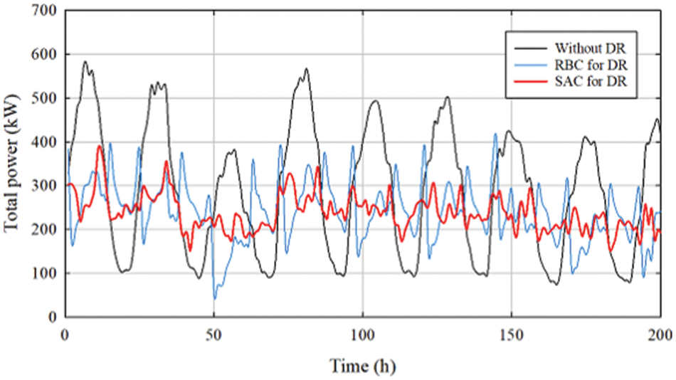
Figure 7: The partial power curve of different control strategies

The electricity demand for one year without DR, RBC, and SAC is shown in Fig. 8a. Without DR, the demand was as high as 1,790,07.85 kW. After using the SAC to control the load, the demand was reduced to 1,480,351.24 kW. Compared with the use of RBC, it saves 14277.54 kW Fig. 8b shows the variance of power demand. The variance of the SAC is much lower than without DR and RBC. It indicates that when the SAC does DR management, the curve has small fluctuations, and it tends to a stable consumption pattern. Neither affects the power supply of the grid and helps reduce the power generation expenditure of the power plant. In each building, the SAC replaces the control strategy of manual rules. They are office, retail, restaurant, and multi-family. The performance of the SAC in office, retail, and Multi-family is worse than the RBC. Still, it is inferior to RBC in a restaurant because the PV array is not installed, and the electricity demand is low.

Figure 8: (a) is the total power in different control strategies and (b) is their variance

The control action curve of the SAC and the RBC in the office is shown in Fig. 9b. The red curve in the figure is the Action of the SAC controlling the cooling storage device to store or release the cooling. The blue curve is the Action of the SAC controlling the DHW storage device to store or release DHW. Compared with the office in Fig. 9a, when the time is 150 h, the power demand of the office is at the peak, and the demand needs to be reduced at this time. The SAC reduces the demand for electrical energy by controlling the cooling storage device or DHW storage device to reduce or increase release. The action values in the picture are all releasing cooling and DHW, reducing the building's energy consumption. The RBC is a manually set action value. During 9:00–21:00, the action value of 0.08 is executed every hour to release cooling or DHW. During 22:00–8:00, the cooling and DHW of 0.091 action value storage are stored every hour. After nine buildings, all use the SAC as the load control strategy, except that the RBC in building 2 is better than the SAC control strategy, the stability of users’ power demand has been improved, as shown in Fig. 9c.

Figure 9: (a) is the power demand of different building types, (c) is the variance of each buildings and (b) is the control curve of the SAC and the RBC in office

Electricity price is one of the influencing factors that affect the electricity demand of users. When the user's electricity demand exceeds the peak of the grid, the power company will increase the price of electricity to allow users to reduce the use of electricity to make the power supply of the grid more stable. Under this policy of changing electricity prices, avoiding electricity use during periods of high electricity prices can reduce costs. For example, the RBC changed the power consumption strategy based on manually set rules, saving 23477.43 dollars. Using the SAC saves 1112.22 dollars, as shown in Fig. 10a.

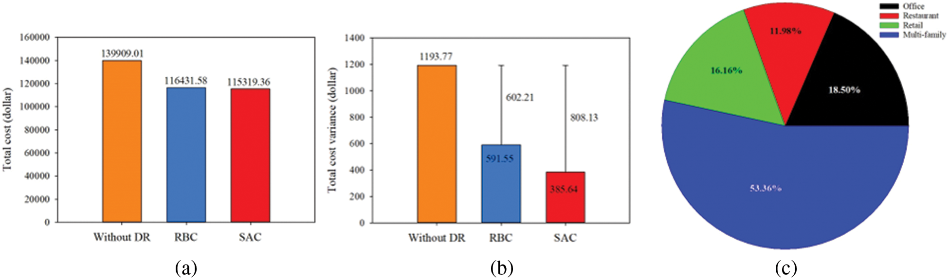
Figure 10: (a) is the total cost in different control strategies, while (b) is their variance, (c) is the distribution of different types of buildings

The variance of Total cost is shown in Fig. 10b. The SAC is more stable in electricity expenditure and will have better savings in future expenditure strategies. The electricity expenditure of different types of buildings is shown in Fig. 10c. The highest is 53.36% for multi-family. This shows that the use of the SAC as a load control strategy for residential users can save users’ electricity expenditures while meeting the cooling and DHW required by users.

5  Conclusion and Future Works

In summary, this paper uses Citylearn as the research environment to allow the SAC to learn and optimize control strategies. After the SAC passes the training, it can make correct actions based on the State of the environment, such as controlling equipment to store or release energy and achieving real-time DR management for controlling load. Reduce the power supply pressure on the power grid during the peak period of power consumption. On the contrary, the stored energy is turned on during the valley period to avoid using it during the peak period. In this way, the user's daily power consumption curve is smoothed. While saving energy and reducing emissions, it provides users with a comfortable living environment. This paper is to control the corresponding equipment of the building through the SAC to make full use of power resources, energy-saving, and emission reduction. The SAC has a good performance in this project, but there are certain hidden dangers. 1) The SAC neural network has a simple structure and can easily be attacked by adversarial learning to make wrong control. 2) The SAC can only be effective for particular buildings and is not very effective in transfer learning. The future research direction is to solve the above two problems.

Funding Statement: This research is supported by Jeollannam-do (2022 R&D supporting program operated by Jeonnam Technopark) and financially supported by the Ministry of Trade, Industry and Energy (MOTIE) and Korea Institute for Advancement of Technology (KIAT) under the research project: “National Innovation Cluster R&D program” (Grant Number: 1415175592 & P0016223).

Conflicts of Interest: The authors declare that they have no conflicts of interest to report regarding the present study.

References

1. T. Logenthiran, D. Srinivasan and T. Z. Shun, “Demand side management in smart grid using heuristic optimization,” IEEE Transactions on Smart Grid, vol. 3, no. 3, pp. 1244–1252, 2012.
2. J. S. Vardakas, N. Zorba and C. V. Verikoukis, “A survey on demand response programs in smart grids: Pricing methods and optimization algorithms,” IEEE Communications Surveys and Tutorials, vol. 17, no. 1, pp. 152–178, 2015.
3. T. Hong, Z. Wang, X. Luo and W. Zhang, “State-of-the-art on research and applications of machine learning in the building life cycle,” Energy and Buildings, vol. 212, pp. 109831, 2020.
4. V. Mnih, K. Kavukcuoglu, D. Silver, A. Graves, I. Antonoglou et al., “Playing atari with deep reinforcement learning,” arXiv preprint arXiv:1312.5602, 2013.
5. Y. Hu, W. Li, K. Xu, T. Zahid, F. Qin et al., “Energy management strategy for a hybrid electric vehicle based on deep reinforcement learning,” Applied Sciences, vol. 8, no. 2, pp. 187, 2018.
6. J. Schulman, S. Levine, P. Abbeel, M. Jordan and P. Moritz, “Trust region policy optimization,” in Proc. of the 32nd Int. Conf. on Machine Learning (ICML), Lille City, France, pp. 1889–1897, 2015.
7. J. Schulman, F. Wolski, P. Dhariwal, A. Radford and O. Klimov, “Proximal policy optimization algorithms,” arXiv preprint arXiv:17006347, 201
8. V. Mnih, A. P. Badia, M. Mirza, A. Graves, T. Lillicrap et al., “Asynchronous methods for deep reinforcement learning,” in Proc. of the 33nd Int. Conf. on Machine Learning (ICML), New York City, NY, USA, pp. 1928–1937, 2016.
9. T. P. Lillicrap, J. J. Hunt, A. Pritzel, N. Heess, T. Erez et al., “Continuous control with deep reinforcement learning,” in Int. Conf. on Learning Representations (ICLR), San Juan City, PR, USA, pp. 1–14, 2016.
10. S. Fujimoto, H. V. Hoof and D. Meger, “Addressing function approximation error in actor-critic methods,” in Proc. of the 35nd Int. Conf. on Machine Learning (ICML), Stockholm City, Sweden, pp. 1587–1596, 2018.
11. T. Haarnoja, A. Zhou, P. Abbeel and S. Levine, “Soft actor-critic: Off-policy maximum entropy deep reinforcement learning with a stochastic actor,” in Proc. of the 35nd Int. Conf. on Machine Learning (ICML), Stockholm City, Sweden, pp. 1856–1865, 2018.
12. T. Haarnoja, A. Zhou, K. Hartikainen, G. Tucker, S. Ha et al., “Soft actor-critic algorithms and applications,” CoRR, abs/1805905, 2018.
13. J. R. Vázquez-Canteli, S. Dey, G. Henze and Z. Nagy. “CityLearn: Standardizing research in multi-agent reinforcement learning for demand response and urban energy management,” CoRR, abs/2012.10504, 2020.
14. J. R. Vázquez-Canteli and Z. Nagy, “Reinforcement learning for demand response: A review of algorithms and modeling techniques,” Applied Energy, vol. 235, pp. 1072–1089, 2019.
15. D. Du and M. Fei, “A two-layer networked learning control system using actor-critic neural network,” Applied Mathematics and Computation, vol. 205, no. 1, pp. 26–36, 2008.
16. H. Kazmi, S. D'Oca, C. Delmastro, S. Lodeweyckx and S. P. Corgnati, “Generalizable occu-pant-driven optimization model for domestic hot water production in NZEB,” Applied Energy, vol. 175, pp. 1–15, 20
17. A. Arif, M. Babar, I. Ahamed, E. AlAmmar, H. P. Nguyen et al., “Online scheduling of plug-in vehicles in dynamic pricing schemes,” Sustainable Energy, Grids and Networks, vol. 7, pp. 25–36, 2016.
18. C. Guan, Y. Wang, X. Lin, S. Nazarian and M. Pedram, “Reinforcement learning-based control of residential energy storage systems for electric bill minimization,” in 2015 12th Annual IEEE Consumer Communications and Networking Conf. (CCNC), Las Vegas City, NV, USA, pp. 637–642, 2015.
19. X. Qi, G. Wu, K. Boriboonsomsin, M. J. Barth and J. Gonder, “Data-driven reinforcement learning-based real-time energy management system for plug-in hybrid electric vehicles,” Transportation Research Record, vol. 2572, no. 1, pp. 1–8, 2016.
20. S. Liu and G. P. Henze, “Experimental analysis of simulated reinforcement learning control for active and passive building thermal storage inventory: Part 1. theoretical foundation,” Energy and Buildingss, vol. 38, no. 2, pp. 142–147, 2006.
21. O. D. Somer, A. Soares, K. Vossen, F. Spiessens, T. Kuijpers et al., “Using reinforcement learning for demand response of domestic hot water buffers: A real-life demonstration,” in 2017 IEEE PES Innovative Smart Grid Technologies Conf. Europe (ISGT-Europe), Turin City, Italy, pp. 1–7, 2017.
22. Y. W. Xie, D. Xie, Y. Zou, D. Zhang, Z. Sun et al., “Deep reinforcement learning for smart home energy management,” IEEE Internet of Things Journal, vol. 7, no. 4, pp. 2751–2762, 2020.
23. C. Zhang, S. R. Kuppannagari, C. Xiong, R. Kannan and V. K. Prasanna, “A cooperative multi-agent deep reinforcement learning framework for real-time residential load scheduling,” in Proc. of the Int. Conf. on Internet of Things Design and Implementation, Montreal City, QC, Canada, pp. 59–69, 2019.
24. E. Mocanu, D. Mocanu, P. Nguyen, A. Liotta, M. Webber et al., “Online building energy optimization using deep reinforcement learning,” IEEE Transactions on Smart Grid, vol. 10, no. 4, pp. 3698–3708, 2019.
25. H. Li, Z. Wan and H. He. “Real-time residential demand response,” IEEE Transactions on Smart Grid, vol. 11, no. 5, pp. 4144–4154, 2020.

This work is licensed under a Creative Commons Attribution 4.0 International License, which permits unrestricted use, distribution, and reproduction in any medium, provided the original work is properly cited.