| Computers, Materials & Continua DOI:10.32604/cmc.2022.029315 | |
| Article |
Wind Turbine Efficiency Under Altitude Consideration Using an Improved Particle Swarm Framework
1Department of Applied Mechanical Engineering, College of Applied Engineering, Muzahimiyah Branch, King Saud University, P.O. BOX 800, Riyadh, 11421, Saudi Arabia
2Department of Applied Electrical Engineering, College of Applied Engineering, Muzahimiyah Branch, King Saud University, P.O. BOX 800, Riyadh, 11421, Saudi Arabia
3Department of Information Science, College of Applied Computer Sciences, Muzahimiyah Branch, King Saud University, P.O. BOX 800, Riyadh, 11421, Saudi Arabia
*Corresponding Author: Haykel Marouani. Email: hmarouani@ksu.edu.sa
Received: 01 March 2022; Accepted: 06 May 2022
Abstract: In this work, the concepts of particle swarm optimization-based method, named non-Gaussian improved particle swarm optimization for minimizing the cost of energy (COE) of wind turbines (WTs) on high-altitude sites are introduced. Since the COE depends on site specification constants and initialized parameters of wind turbine, the focus was on the design optimization of rotor radius, hub height and rated power. Based on literature, the COE is converted to the Saudi Arabia context. Thus, the constrained wind turbine optimization problem is developed. Then, non-Gaussian improved particle swarm optimization is provided and compared with the conventional particle swarm optimization for solving the optimization design in wind turbine efficiency under different altitudes ranging from 2500 to 4000 m. The results show that as altitude rises, the optimal rotor radius grows, but the optimal hub height and rated power drop, resulting in an increase in COE. Further, the non-Gaussian method display a faster convergence compared to the classical particle swarm optimization. These findings will be useful as a reference for wind turbine design at high altitudes. Thus, it could be employed to optimize the initialized parameter of wind turbine for the planned and largest wind farm in Saudi Arabia in Dumat Al-Jandal selected site.
Keywords: Wind turbine; high altitude; energy cost; particle swarm optimization; Lévy distribution
New installations of wind power in 2020 exceeded 90 GW (86.9 GW onshore and 6.1 GW offshore), up 53% from the previous year, bringing total installed capacity to 743 GW, up 14% from the previous year [1]. Although, most of the WTs are within the low-altitude wind sites, the need for erecting WTs at high-altitude wind sites has risen dramatically. In China, for example, WTs have been installed at locations ranging from 0 to 4000 meters [2]. Thus, the impact of high altitude site’s on the economic benefit should be fully considered. It is known that the altitude of the site has considerable impact on environmental characteristics such as, air density, air pressure, air temperature, humidity, solar radiation, etc. Consequently, the high altitude wind site has a notable impact on the WTs’ energy production and production cost. Special designs should be constructed for WTs at sites with altitudes greater than 2000 m. According to detailed study [3,4], special designs should be considered on the wind blade, generator, converter, control system, and lighting protection, for the WTs to be safely operated at high-altitude sites with low air pressure, low air temperature, and high solar radiations [5].
The techno-economic investigation of the wind power farms can be view from economic or engineering stand point. COE is one of the most widely utilized evaluation criteria [2,6,7]. It refers to the cost of producing 1 KWh electric energy, including annual energy production cost and annual energy production as defined in the “National Renewable Energy Laboratory Wind Turbine Design Cost and Scaling Model” study [8]. The cost of producing wind energy at high-altitude sites is higher than any terrain when wind turbine is installed. Furthermore, the complicated topography of high altitude sites adds to the expense, as it makes turbine conveyance, installation, and maintenance more difficult [5]. Other economic factors can be utilized to determine a wind farm’s economic viability. They may include the use of net present value [9,10] (i.e., the present value of the incoming and outgoing cash flow from the investment, and thus shows the total benefit to be derived from the investment in a project), the pay-back period [11,12] (i.e., the period in which the cost of the initial investment is recovered through annual cash flows), and the internal rate of return [13,14] (i.e., the rate of return or internal rate of return of an investment).
The techno-economic investigation of wind farm depends on the WT design. Recently, the design optimization of WTs has narrowed into three study directions which can be identified in the relevant studies in literature: control design optimization, blade design optimization, and site-specific design optimization. Control design optimization, a prevalent approach in the wind energy industry for increasing energy production efficiency, uses the predicted effective wind speed or wind direction as an input with advanced controls that can be adopted to torque and yaw system [15]. Despite its cost-effectiveness, control design optimization reached their maximum capabilities and has only yielded a small profit. For example, a previous study found that refining the control architecture of the WT deployed at the high-altitude site increased energy production by about 0.8 percent [16]. The wind blades are considered as the most important and expensive part in the wind turbine. Blade design optimization is determined by the aerodynamic geometry of blade airfoil [17,18] and interact with the blade load and the blade mass. The effectiveness of blade design optimization in boosting energy production efficiency has been demonstrated [19,20]. The site-specific design optimization deals with three fundamental concepts [2,6,7]: the objective function, the designed parameters, and the optimization method. Objective function depends on the techno-economic problem formulation. Designed parameters include the WT’s most critical factors as rated power, rated wind speed, tip speed ratio, rotor size, and hub height. The widely used optimization methods are particle swarm optimization (PSO) [2], Yin-Yan pair optimization [7], Pareto front [6], genetic algorithm [6], chaotic search strategy [21] and fuzzy algorithm [22].
This research focuses on optimizing WTs for high-altitude sites, with focus on the energy cost issue. In this paper, we first address the high-altitude site specific design optimization of WTs linking energy cost and wind turbine power. Then, we present an objective optimization approach based on a non-Gaussian PSO for optimizing WTs’ three design parameters which are rotor radius, hub height, and wind turbine rated power. Finally, the proposed method is tested and discussed, with the results being for further use to farm WTs designers.
The remaining sections are arranged as follows: in Section 2, the wind turbine efficiency at high-altitude sites is formulated. Section 3 presents the PSO formulation based on the non-Gaussian Levy distribution function and the expression of the energy-cost optimization problem. The effectiveness of the proposed approach is demonstrated through a detailed examination in Section 4. Finally, Section 5 concludes the study.
2 Wind Turbine Efficiency Problem
Wind turbine efficiency depends essentially on minimizing the annual production cost (APC) [SAR] while maximizing the annual energy production AEP [kWh]. Song et al. [7] rewrite this multi-objective energy-cost problem as a minimization of a single function, named COE [SAR/kWh], which is expressed as the ratio of APC to AEP:
Adapting the techno-economic model developed by the National Renewable Energy Laboratory of the United States Department of energy [8] to the Saudi Arabia context, and as reported by Song et al. [2], APC depends on the initial capital cost (ICC) [SAR], the fixed charge rate (FCR) [-] and annual operating cost (replacement cost, land leasing cost, and operation and maintenance cost) AOC [SAR]:
The ICC is governed by the cost of wind turbine CTurbine [SAR] and the cost of infrastructure CInfrastructure [SAR]:
CTurbine and CInfrastructure can be expressed considering the impact of altitude factors (Rotor radius R [m], turbine altitude Haltitude [m], hub height H [m] and rated power Pr [MW]) as follows:
The AOC model is expressed according to [2]:
AEP expression is based on the power curve [23] and the Weibull distribution model [24,25]. The difference between onshore and offshore WTs are denoted on the scale parameter and shape parameter of the Weibull distribution. The final expression of AEP is:
where 8760 represents a factor, η is the total loss of energy, and Pm is the hourly energy production [kWh].
The hourly energy production depends on Haltitude, the maximum power coefficient Cpmax [-], the wind speed function f(V) [m/s], the cut-in wind speed Vcut-in [m/s], the rated wind speed Vr [m/s], the cut-off wind speed Vcut-off [m/s], and temperature T [K]. Pm is then defined by the following equation:
where f(V) is the Weibull distribution that models the wind resource parameters.
where k is the shape factor, and c is the scale factor.
where k0 and c0 are the value of k and c at the reference height H0 respectively. α is the wind shear coefficient (Hellmann exponent) [26].
where Vm is the mean wind speed at the reference height, and Γ(-) is the gamma function.
The rated wind speed is given by:
where ρ is the air density [kg.m−3], which changes with altitude and temperature T. According to the ideal gas law, air density is determined by the following equation:
where P is the pressure [Pa], P0 is the standard pressure [101.325 KPa] and T0 is the standard temperature [288.15 K] under standard conditions (sea level, 15 degrees Celsius).
In line with the US Standard Atmosphere, up to an altitude of 11,000 m, temperature decreases linearly with altitude according to the following equation (0.0065 is the lapse rate coefficient):
Finally, the COE expression presented in this work depends on 9 fixed-design parameters {η, α, Cpmax, Vcut-in, Vcut-off, Vm, FCR, k0, H0} and on 4 variables parameters {R, H, Haltitude, Pr}. Otherwise, at a certain altitude Haltitude, COE can be optimized (minimized) by choosing the appropriate rotor radius (R), hub height (H), and rated power (Pr), subject to upper and lower bounds due to technical considerations. In order to formulate this wind turbine efficiency problem, the fitness function and structure constraints are presented as follows:
PSO has been ingrained by scientific researchers and has been continually improved in vast optimization problems. The PSO algorithm finds the best global by combining individual and group experience, and is easy to achieve. Nonetheless, PSO’s major flaw is that during the iterative phase, all solutions are optimized and searched, resulting in premature convergence and local convergence [27]. The improved non-Gaussian PSO algorithm (ING-PSO) will fix this deficiency.
3.1 Particle Swarm Optimization Algorithm
PSO is a stochastic optimization algorithm initially proposed by Kennedy and Eberhart in 1995 [28] and nowadays widely used in multi-objective optimization problems [29]. Based on swarm intelligence, potential solutions are named particles.
Let consider a D-dimension problem and let set N particles. The position of the ith particle is defined by:
Each particle has to ‘fly’ with a specified velocity to improve its previous position (solution) based on these expressions:
where (c1, c2) are acceleration factors and (r1, r2) are random numbers between 0 and 1. k denote the current iteration number, and
ci factors point out the learning process of particles, by developing themselves and by learning from the experience of the others. Acceleration factors contribute to avoid falling into a local optimum solution and to a better search for the best global one. Random ri numbers are used to simulate the random and unconstrained particles’ movement. Inertia factor is linked to the rate exploration of the solution space. Great value of
The inertia weight is updated according to the following equation:
where wmax and wmin are the maximum and minimum inertial weight. Imax is the maximum number of iterations.
The basic PSO steps are summarized as follows [29,31]:
Step 1: Initialize the PSO constants (N, D, c1, c2, wmax, wmin, Imax).
Step 2: Randomly set the initial position Xi0 and initial velocity Vi0.
Step 3: Allow the particle swarm to find the best results.
Step 4: Evaluate the fitness of each particle.
Step 5: Update the best position Pi of each individual particle.
Step 6: Update the particle velocity and position.
Step 7: The PSO method is stopped and the last global best locations are the solution if the end condition (limit number of iterations reached or fitness value less than initially defined) is met.. If the end condition is not met, go to step 3.
3.2 Improved Non-Gaussian Particle Swarm Optimization Algorithm
Traditional PSO algorithm has limitations [32–35]: it leads to premature convergence phenomenon, which cannot perform a good global search and fall into the local solution convergence situation. In order to fix this deficiency, new research combine PSO with other evolutionary algorithms [36–40] or try to express new formulations of the inertia coefficient, acceleration coefficient, velocity or position updating [41]. In this paper, the Levy distribution, a non-Gaussian random distribution, is combined with PSO. This choice is justified because the Levy distribution can realize the multi-step hopping of particles in the search space to achieve the purpose of improving search efficiency [27,42,43].
Levy flight is a random search process that follows the levy distribution [44]. This is a short-distance local search and occasionally long-distance global search, whose step size and time follow Levy distribution. Because Levy flight’s local and global search capabilities are more prominent, it is more suitable for application in the field of optimization. Levy distribution can be defined as:
where μ is the location parameter (minimum step size) and cL is the scale parameter.
In a non-Gaussian particle swarm optimization, the new position of each particle is updated using the following equation:
γ is a scaling parameter for the solved problem D that determines the step size:
In our case,
L(w) represents the Levy distribution.
The N-sample generated is expressed as:
where η is derived from the normal distribution η|N(0,σ²).
Note that optimization algorithm must provide solutions within a feasible search space. The wind turbine efficiency problem (see Section 2) includes inequality constraints with upper and lower bounds. For this reason, penalties are added to the classical and improved non-Gaussian particle swarm optimization algorithm. The penalty function (Max, Min) constraint handling method [29,45,46] is used to handle the equal inequality constraints. Small values ε are added to adapt the strict inequality constraints into equal ones. Thus, the penalty values
4 Application, Results and Discussion
To demonstrate the capability of the proposed improved PSO approach, this work investigates the COE performance of the WTs. PSO and improved Non-Gaussian PSO algorithms are used to optimize the design parameters of WTs corresponding to the minimum COE at different altitudes. First, the variation trends of the optimal parameters and COE with altitude are analyzed, and then the efficiency of the improved Non-Gaussian PSO is discussed.
PSO and ING-PSO-based algorithms parameters includes the site specification constants, the initialized parameter of WT and the algorithms parameters (Tab. 1). The site specification constants are taken for one of the highest and windiest region in Kingdom of Saudi Arabia, which is Abha region. According to https://globalwindatlas.info website, the annual wind speed is equal to 7.25, 8.49, 9.33 and 9.86 m/s at 50, 100, 150 and 200 m, respectively. The reference height is set at 50 m, the shape factor k0 is a typical value of 2. Then the scale factor c0 can be obtained by Eq. (12). The mean wind speed Vm at the reference height is 7.25 m/s. Because the wind shear coefficient is small on high-altitude flat area, the wind shear coefficient is 0.1 [47]. Rated wind speed is obtained by combining Eqs. (13)–(15). Scale and shape factors are deducted by using Eqs. (10) and (11), respectively.
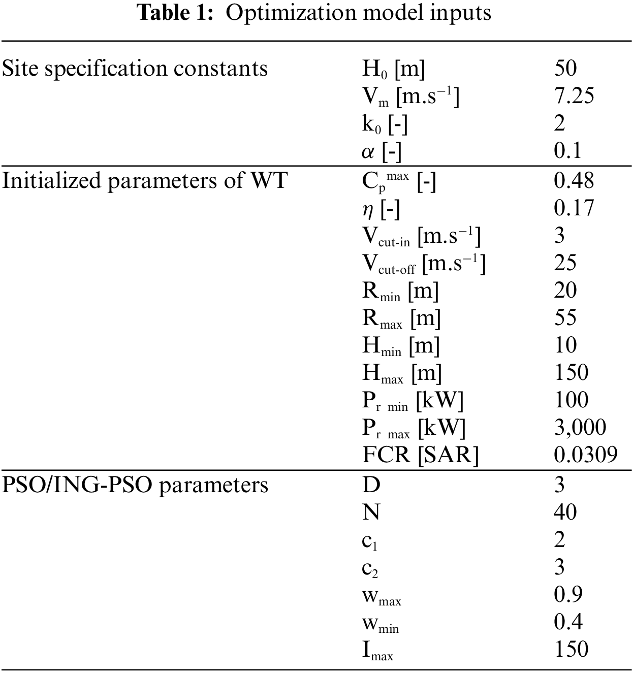
The initialized parameters of WT are choosing according to literature investigating large-scale variable-speed WT [2]. Considering that the cost model used is aimed for large-scale WTs on high-altitude areas, the range of R is 20–55 m, the range of H is 10–150 m and the range of Pr is 100–3000 kW, the cut-in and cut-off wind speeds are 3 and 25 m/s, respectively. The maximum power coefficient is set at 0.48. Hourly energy production is obtained by using Eqs. (8) and (9). AEP and AOC are calculated based on Eqs. (6) and (7), respectively. ICC is estimated by using Eqs. (4) and (5) and then Eq. (3). The calculation of APC is made by Eq. (2), which allows for correct estimation of COE by using Eq. (1).
The algorithms parameters are the problem dimension, the population size, the acceleration factors, the maximum and minimum inertia factors, and the maximum number of iterations.
The identified and optimized values {R, H, Pr} are obtained for a fixed altitude Haltitude. The initial altitude value is set at 2500 m, increasing by 500 m for each new optimization calculation, the maximum altitude is 4000 m.
The discussed methods were implemented in MATLAB R2021a, and their performances were tested using a laptop computer with a core i7-4700MQ central processing unit at 2.4 GHz, with 8 Gigabytes of Random Access Memory. Fig. 1 depict the COE convergence trend at different high altitudes. We notice that improved Non-Gaussian PSO converges faster than PSO for all altitude cases (64–70 iterations vs. 92–100 iterations). PSO starts with an initial COE of 0.1966215 SAR/KWh and converges to 0.1966153 SAR/KWh. Improved Non-Gaussian PSO starts with an initial COE of 0.1966208 SAR/KWh and converges to 0.1966151 SAR/KWh. Fig. 2 describes the variation trend of COE with altitude. ING-PSO shows that COE increase linearly with altitude increase. At the altitude of 2500 m, the COE is 0.19661522 SAR/KWh and reach 0.21396282 SAR/KWh at 4000 m, which represent an increase by 9.22%.
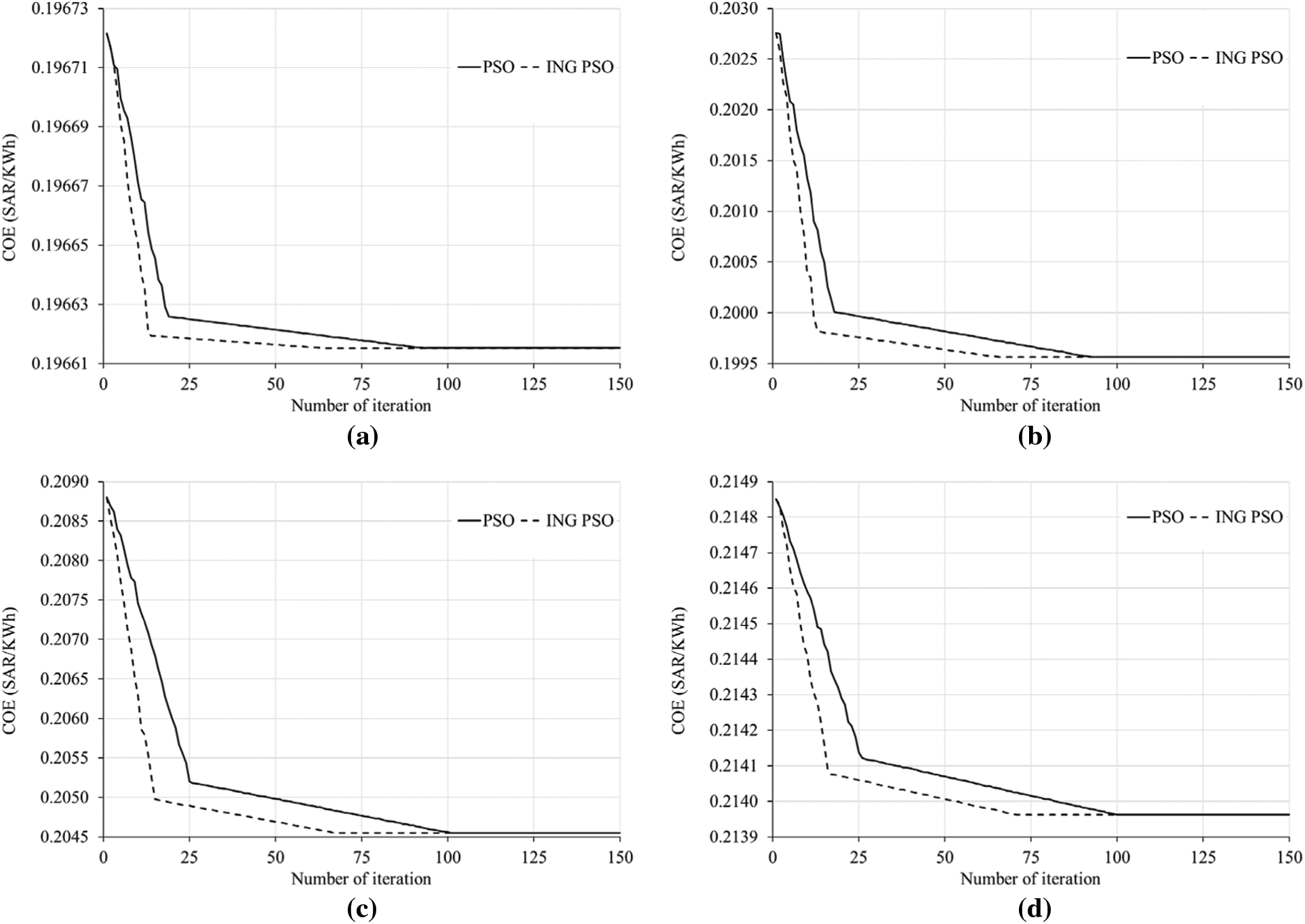
Figure 1: COE convergence trend at different altitudes: (a) 2500 m, (b) 3000 m, (c) 3500 m, (d) 4000 m
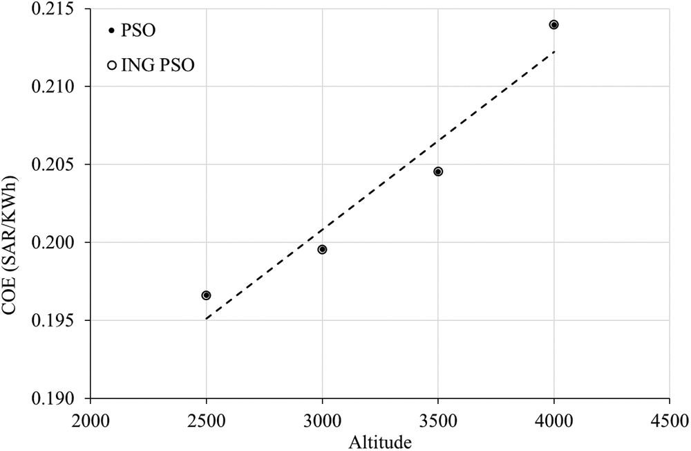
Figure 2: Optimal COE evolution with altitude
Tab. 2 shows the improvement that ING-PSO is bringing compared to classical PSO. The results can be considered as the same but with fast convergence speed.

The convergence trend of R, H and Pr at different altitudes using PSO and improved Non-Gaussian PSO algorithms are depicted in Figs. 3–5, respectively. As for the COE convergence trend, the improved Non-Gaussian PSO converges faster than PSO for all altitude cases at the same range of iteration values (64–70 iterations vs. 92–100 iterations). Tab. 3 summarizes the optimal design parameters and corresponding optimal COE at different altitudes. Both algorithms show the same finding: The rotor radius grows as altitude rises, while hub height and rated power decrease.
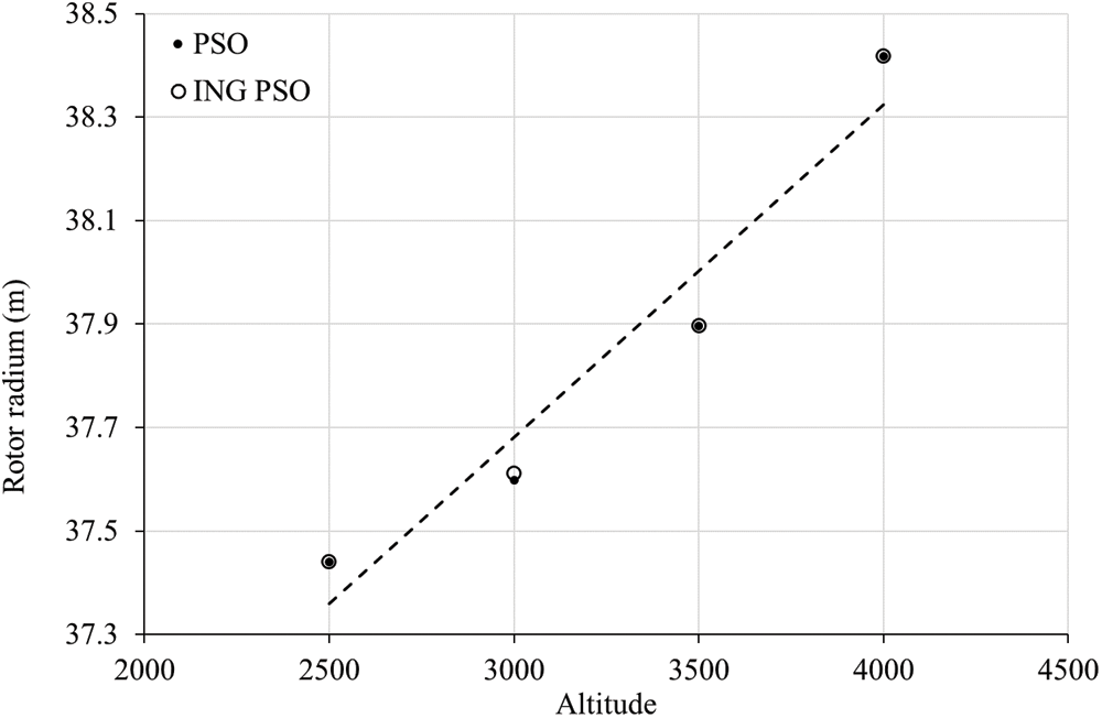
Figure 3: Optimal R evolution with altitude
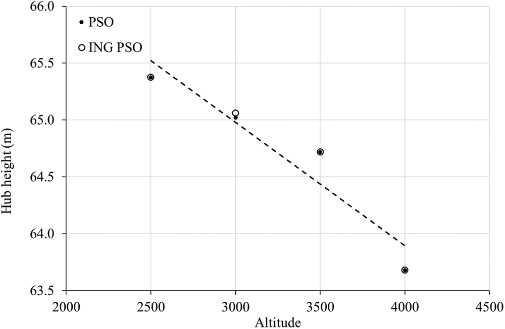
Figure 4: Optimal H evolution with altitude
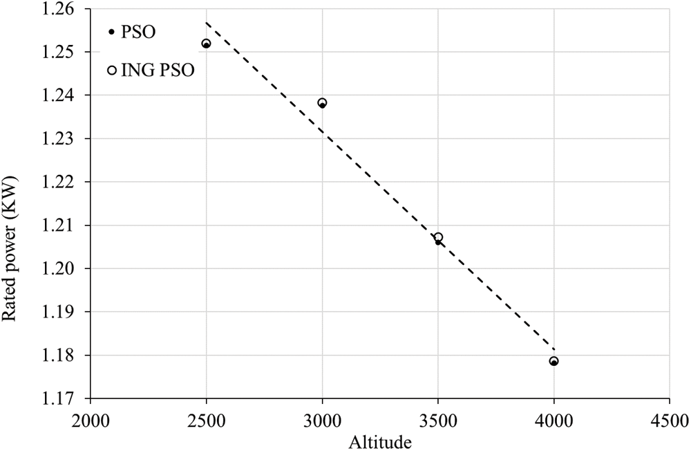
Figure 5: Optimal Pr evolution with altitude

At the altitude of 2500 m, R is 37.44013343 m and reach 38.41780315 m at 4000 m, which represent an increase by 0.97767 m (2.61%). At the altitude of 2500 m, H is 65.37496143 m and reach 63.68161671 m at 4000 m, which represent a decrease by 2.59%. At the altitude of 2500 m, Pr is 1.251938064 MW and reach 1.178612624 MW at 4000 m, which represent a decrease by 5.86%. As the increase of altitude decreases air density, it leads to the drop of energy production. As a result, in order to keep the same rated power, the rotor radius must be expanded, resulting in a rise in wind turbine costs. Further, high altitude sites are associated with higher infrastructure cost and WTs installation cost.
In this study, two optimization algorithms were proposed for wind turbine design optimization on high-altitude: a well-established PSO approach and a most recent technique called non-Gaussian improved PSO. Both optimizations search for the optimal rotor radius, hub height and rated power at different altitudes ranging from 2500 to 4000 m. Result comparison have proven that the ING-PSO has slight better performance for the same final results. It is the first work that ING-PSO is applied to optimize the wind turbine efficiency under altitude consideration. ING-PSO has the fast convergence speed and a slightly better result (COE is improved by less than 0.0003%). Regarding the WT design, we conclude that with the increase of altitude from 2500 to 4000 m, the optimal rotor radius increases from 37.44013343 to 38.41780315 m (+2.61%), the optimal hub height decreases from 65.37496143 m to 63.68161671 (–2.59%), the optimal rated power decreases from 1.251938064 to 1.178612624 MW (5.86%), and the COE increases from 0.19661522 to 0.21396282 SAR/KWh (+8.8%).
This work presents the first WT efficiency investigation for the Saudi Arabia context, as Saudi Arabia plans to generate 60 GW of renewable energy by 2030 of which 20 GW from wind. In future work, we plan to optimize the initialized parameter of WT at Dumat Al-Jandal site, which is a 415 MW onshore wind farm development that will become the Saudi Arabia’s first wind power source and the largest wind farm in the Middle East region.
Funding Statement: The authors extend their appreciation to the Researchers Supporting Project number (RSP2022R515), King Saud University, Riyadh, Saudi Arabia for funding this research work.
Conflicts of Interest: The authors declare that they have no conflicts of interest to report regarding the present study.
References
1. J. Lee and F. Zhao, “Global wind report 2021,” Global Wind Energy Council, 2021. [Google Scholar]
2. D. Song, J. Liu, J. Yang, M. Su, S. Yang et al., “Multi-objective energy-cost design optimization for the variable-speed wind turbine at high-altitude sites,” Energy Conversion and Management, vol. 196, no. 6–7, pp. 513–524, 2019. [Google Scholar]
3. C. Wang and R. G. Prinn, “Potential climatic impacts and reliability of very large-scale wind farms,” Atmospheric Chemistry and Physics, vol. 10, no. 4, pp. 2053–2061, 2010. [Google Scholar]
4. C. Wang and R. G. Prinn, “Potential climatic impacts and reliability of large-scale offshore wind farms,” Environmental Research Letters, vol. 6, no. 2, pp. 25101, 2011. [Google Scholar]
5. Y. Hu, W. Huang, J. Wang, S. Chen and J. Zhang, “Current status, challenges, and perspectives of Sichuan’s renewable energy development in Southwest China,” Renewable and Sustainable Energy Reviews, vol. 57, no. 4, pp. 1373–1385, 2016. [Google Scholar]
6. M. A. Mellal and M. Pecht, “A multi-objective design optimization framework for wind turbines under altitude consideration,” Energy Conversion and Management, vol. 222, pp. 113212, 2020. [Google Scholar]
7. D. Song, J. Liu, J. Yang, M. Su, Y. Wang et al., “Optimal design of wind turbines on high-altitude sites based on improved Yin-Yang pair optimization,” Energy, vol. 193, no. 3, pp. 116794, 2020. [Google Scholar]
8. L. Fingersh, M. Hand and A. Laxson, Wind turbine design cost and scaling model. in National Renewable Energy Laboratory Technical Report, Golden, CO, USA, pp. 1–43, 2006. [Google Scholar]
9. D. Petković, S. Shamshirband, A. Kamsin, M. Lee, O. Anicic et al., “Survey of the most influential parameters on the wind farm net present value (NPV) by adaptive neuro-fuzzy approach,” Renewable and Sustainable Energy Reviews, vol. 57, no. 8, pp. 1270–1278, 2016. [Google Scholar]
10. J. Wyrobek, Ł. Popławski and M. Dzikuć, “Analysis of financial problems of wind farms in Poland,” Energies, vol. 14, no. 5, pp. 1239, 2021. [Google Scholar]
11. L. Castro-Santos and A. Filgueira-Vizoso, “A software for calculating the economic aspects of floating offshore renewable energies,” International Journal of Environmental Research and Public Health, vol. 17, no. 1, pp. 218, 2020. [Google Scholar]
12. C. Mattar and M. C. Guzmán-Ibarra, “A techno-economic assessment of offshore wind energy in Chile,” Energy, vol. 133, no. 9, pp. 191–205, 2017. [Google Scholar]
13. L. Castro-Santos, A. R. Bento, D. Silva, N. Salvação and C. G. Soares, “Economic feasibility of floating offshore wind farms in the North of Spain,” Journal of Marine Science and Engineering, vol. 8, no. 1, pp. 58, 2020. [Google Scholar]
14. S. S. Ahmad, A. Al Rashid, S. A. Raza, A. A. Zaidi, S. Z. Khan et al., “Feasibility analysis of wind energy potential along the coastline of Pakistan,” Ain Shams Engineering Journal, vol. 13, no. 1, pp. 101542, 2022. [Google Scholar]
15. J. M. Hegseth, E. E. Bachynski and J. R. R. A. Martins, “Integrated design optimization of spar floating wind turbines,” Marine Structures, vol. 72, no. 9, pp. 102771, 2020. [Google Scholar]
16. D. Song, J. Yang, Z. Cai, M. Dong, M. Su et al., “Wind estimation with a non-standard extended Kalman filter and its application on maximum power extraction for variable speed wind turbines,” Applied Energy, vol. 190, no. 4, pp. 670–685, 2017. [Google Scholar]
17. K. Yang, “Geometry design optimization of a wind turbine blade considering effects on aerodynamic performance by linearization,” Energies, vol. 13, no. 9, pp. 2320, 2020. [Google Scholar]
18. M. Z. Dosaev, L. A. Klimina, B. Y. Lokshin and Y. D. Selyutskiy, “On wind turbine blade design optimization,” Journal of Computer and Systems Sciences International, vol. 53, no. 3, pp. 402–409, 2014. [Google Scholar]
19. S. L. Lee and S. J. Shin, “Wind turbine blade optimal design considering multi-parameters and response surface method,” Energies, vol. 13, no. 7, pp. 1639, 2020. [Google Scholar]
20. J. Zhu, X. Cai and R. Gu, “Multi-objective aerodynamic and structural optimization of horizontal-axis wind turbine blades,” Energies, vol. 10, no. 1, pp. 101, 2017. [Google Scholar]
21. R. M. Rizk-Allah, A. E. Hassanien and D. Song, “Chaos-opposition-enhanced slime mould algorithm for minimizing the cost of energy for the wind turbines on high-altitude sites,” ISA Transactions, vol. 121, no. 15, pp. 191–205, 2021. [Google Scholar]
22. G. Abdelmassih, M. Al-Numay and A. El Aroudi, “Map optimization fuzzy logic framework in wind turbine site selection with application to the usa wind farms,” Energies, vol. 14, no. 19, pp. 6127, 2021. [Google Scholar]
23. A. A. Teyabeen, F. R. Akkari and A. E. Jwaid, “Power curve modelling for wind turbines,” in 19th Int. Conf. on Computer Modelling & Simulation, Cambridge, UK, 2017. [Google Scholar]
24. A. Sayal, A. P. Singh and D. Aggarwal, “Optimisation of EOQ model with Weibull deterioration under crisp and fuzzy environment,” International Journal of Mathematical Modelling and Numerical Optimisation, vol. 9, no. 4, pp. 400–428, 2019. [Google Scholar]
25. R. P. Covert and G. C. Philip, “An eoq model for items with weibull distribution deterioration,” AIIE Transactions, vol. 5, no. 4, pp. 323–326, 1973. [Google Scholar]
26. G. K. Gugliani, A. Sarkar, C. Ley and V. Matsagar, “Identification of optimum wind turbine parameters for varying wind climates using a novel month-based turbine performance index,” Renewable Energy, vol. 171, no. 4, pp. 902–914, 2021. [Google Scholar]
27. F. Sun, Z. Xu and D. Zhang, “Optimization design of wind turbine blade based on an improved particle swarm optimization algorithm combined with non-gaussian distribution,” Advances in Civil Engineering, vol. 2021, pp. 6699797, 2021. [Google Scholar]
28. J. Kennedy and R. C. Eberhart, “Swarm intelligence,” The Morgan Kaufmann Series in Artificial Intelligence, 1st ed., vol. 1, Burlington, MA, USA: Morgan Kaufmann, pp. 287–318, 2001. [Google Scholar]
29. A. A. Kadkol, “Mathematical model of particle swarm optimization: Numerical optimization problems,” International Series in Operations Research & Management Science, vol. 306, pp. 73–95, 2021. [Google Scholar]
30. H. Marouani, K. Hergli, H. Dhahri and Y. Fouad, “Implementation and identification of preisach parameters: Comparison between genetic algorithm, particle swarm optimization, and Levenberg-Marquardt algorithm,” Arabian Journal for Science and Engineering, vol. 44, no. 8, pp. 6941–6949, 2019. [Google Scholar]
31. H. Marouani and Y. Fouad, “Particle swarm optimization performance for fitting of Lévy noise data,” Physica A: Statistical Mechanics and its Applications, vol. 514, pp. 708–714, 2019. [Google Scholar]
32. J. Too, A. R. Abdullah and N. M. Saad, “A new co-evolution binary particle swarm optimization with multiple inertia weight strategy for feature selection,” Informatics, vol. 6, no. 2, pp. 21, 2019. [Google Scholar]
33. S. S. Aote, M. M. R. Principal and R. L. Malik, “A brief review on particle swarm optimization: Limitations & future directions,” International Journal of Computer Science Engineering, vol. 2, no. 5, pp. 196–200, 2013. [Google Scholar]
34. H. Yu, Y. Gao, L. Wang and J. Meng, “A hybrid particle swarm optimization algorithm enhanced with nonlinear inertial weight and gaussian mutation for job shop scheduling problems,” Mathematics, vol. 8, no. 8, pp. 1355, 2020. [Google Scholar]
35. X. Zhang, L. Jiao, A. Paul, Y. Yuan, Z. Wei et al., “Semisupervised particle swarm optimization for classification,” Mathematical Problems in Engineering, vol. 2014, pp. 832135, 2014. [Google Scholar]
36. L. Sahoo, A. Banerjee, A. K. Bhunia and S. Chattopadhyay, “An efficient GA-PSO approach for solving mixed-integer nonlinear programming problem in reliability optimization,” Swarm and Evolutionary Computation, vol. 19, no. 5, pp. 43–51, 2014. [Google Scholar]
37. M. Sheikhalishahi, V. Ebrahimipour, H. Shiri, H. Zaman and M. Jeihoonian, “A hybrid GA-PSO approach for reliability optimization in redundancy allocation problem,” International Journal of Advanced Manufacturing Technology, vol. 68, no. 1-4, pp. 317–338, 2013. [Google Scholar]
38. H. Shokri-Ghaleh, A. Alfi, S. Ebadollahi, A. Mohammad Shahri and S. Ranjbaran, “Unequal limit cuckoo optimization algorithm applied for optimal design of nonlinear field calibration problem of a triaxial accelerometer,” Measurement, vol. 164, pp. 107963, 2020. [Google Scholar]
39. P. Pant and D. Chatterjee, “Prediction of clad characteristics using ANN and combined PSO-ANN algorithms in laser metal deposition process,” Surfaces and Interfaces, vol. 21, no. 3, pp. 100699, 2020. [Google Scholar]
40. T. Balachander, P. A. Jeyanthy and D. Devaraj, “Combined PSO and IBF algorithm for short term hydro thermal scheduling,” International Journal of Recent Technology and Engineering, vol. 8, no. 4, pp. 418–424, 2019. [Google Scholar]
41. H. Marouani, “Optimization for the redundancy allocation problem of reliability using an improved particle swarm optimization algorithm,” Journal of Optimization, vol. 2021, pp. 6385713, 2021. [Google Scholar]
42. H. Hakli and H. Uǧuz, “A novel particle swarm optimization algorithm with Levy flight,” Applied Soft Computing Journal, vol. 23, no. 3, pp. 333–345, 2014. [Google Scholar]
43. C. Charin, D. Ishak, M. A. A. Mohd Zainuri, B. Ismail and M. K. Mohd Jamil, “A hybrid of bio-inspired algorithm based on Levy flight and particle swarm optimizations for photovoltaic system under partial shading conditions,” Solar Energy, vol. 217, pp. 1–14, 2021. [Google Scholar]
44. E. H. Houssein, M. R. Saad, F. A. Hashim, H. Shaban and M. Hassaballah, “Lévy flight distribution: A new metaheuristic algorithm for solving engineering optimization problems,” Engineering Applications of Artificial Intelligence, vol. 94, no. 5, pp. 103731, 2020. [Google Scholar]
45. L. L. Rodrigues, J. Sebastian Solis-Chaves, O. A. C. Vilcanqui and A. J. S. Filho, “Predictive incremental vector control for DFIG with weighted-dynamic objective constraint-handling method-PSO weighting matrices design,” IEEE Access, vol. 8, pp. 114112–114122, 2020. [Google Scholar]
46. F. Peng, S. Hu, Z. Gao, W. Zhou, H. Sun et al., “Chaotic particle swarm optimization algorithm with constraint handling and its application in combined bidding model,” Computers and Electrical Engineering, vol. 95, no. 8, pp. 107407, 2021. [Google Scholar]
47. W. Werapun, Y. Tirawanichakul and J. Waewsak, “Wind shear coefficients and their effect on energy production,” Energy Procedia, vol. 138, no. 1, pp. 1061–1066, 2017. [Google Scholar]
 | This work is licensed under a Creative Commons Attribution 4.0 International License, which permits unrestricted use, distribution, and reproduction in any medium, provided the original work is properly cited. |