Computers, Materials & Continua
DOI:10.32604/cmc.2022.029467 |  |
| Article | |
NOMA-Based Cooperative Relaying Transmission for the Industrial Internet of Things
Yinghua Zhang1,*, Rui Cao1, Lixin Tian1, Rong Dai2, Zhennan Cao2 and Jim Feng3
1Dawning Information Industry Co., Ltd., Beijing, 100193, China
2Dawning Information Industry Chengdu Co., Ltd., Chengdu, 610041, China
3Amphenol Global Interconnect Systems, San Jose, CA, 95131, US
*Corresponding Author: Yinghua Zhang. Emails: 82774807@qq.com, zhangyh@sugon.com
Received: 04 March 2022; Accepted: 06 June 2022
Abstract: With the continuous maturity of the fifth generation (5G) communications, industrial Internet of Things (IIoT) technology has been widely applied in fields such as smart factories. In smart factories, 5G-based production line monitoring can improve production efficiency and reduce costs, but there are problems with limited monitoring coverage and insufficient wireless spectrum resources, which restricts the application of IIoT in the construction of smart factories. In response to these problems, we propose a hybrid spectrum access mechanism based on Non-Orthogonal Multiple Access (NOMA) cooperative relaying transmission to improve the monitoring coverage and spectrum efficiency. As there are a large number of production lines that need to be monitored in smart factories, it is difficult to realize real-time monitoring of all production lines due to insufficient wireless resources. Therefore, we divide the production lines into high priority and low priority, and introduce cognitive radio technology to increase the number of monitoring production lines. In order to better describe the wireless fading channel environment in the factory, the two-wave with diffuse power (TWDP) channel is discussed to simulate the real factory environment and the outage probability of the secondary production line data transmission is derived in the proposed mechanism. Compared with the traditional mechanism, the proposed transmission mechanism can ensure the continuity of the secondary transmission, greatly reduce the outage probability of the secondary transmission, and improve the efficiency of the monitoring of the production lines.
Keywords: Relay; IIoT; outage probability; NOMA; TWDP; beam-forming
1 Introduction
1.1 New Wireless Technologies
The development of the fifth generation (5G) communication [1,2] has introduced more possibilities to the application of industrial Internet of Things (IIoT) technology in society [3–5]. Compared with the production model of traditional factories, smart factories based on the IIoT can use technologies such as industrial automation and smart sensors to improve factory production efficiency and reduce costs [6]. At the same time, it is also one of the important scenarios for 5G applications [7,8]. In the construction of smart factories, it is of great significance for the automatic monitoring of production lines. It is responsible for monitoring the working conditions of all production lines in the factory to ensure the orderly production of industrial products. However, in the practical application of the IIoT, the scale of the factory makes it impossible to monitor a wide range of production lines. At the same time, the large number of production lines in the factory will cause the problem of shortage of wireless spectrum resources [9]. These problems limit the monitoring of production lines in efficiency, which is the key to application in factory construction.
Non-Orthogonal Multiple Access (NOMA) technology has aroused widespread concern in academia and industry because of its high spectral efficiency [10]. In a traditional Orthogonal Multiple Access (OMA) system, the system allocates different time-frequency resources to each monitoring equipment, and information between monitoring equipment cannot be superimposed on each other. Unlike OMA, multiple monitoring equipment on the same time-frequency resource are served simultaneously by information superimposition, which greatly improves system throughput and spectrum efficiency. At the same time, NOMA has many advantages over OMA systems. For example, it does not rely on Channel State Information (CSI) itself, and can obtain a stable gain in a scenario of high-speed movement [11]. In addition, NOMA can also achieve hands-free access, reduce network latency, and reduce monitoring equipment power consumption. It has broad application prospects in the future with low latency requirements such as intelligent transportation, smart cities and IIoT [12]. At the same time, multi-antenna technology and NOMA can be well combined to significantly improve system performance. At present, Multiple-Input-Multiple-Output (MIMO) NOMA system has become a research hotspot [13]. In addition, the cooperative relay technology is more and more recognized by the academic and industrial circles because of its outstanding advantages in increasing the coverage area of wireless cellular mobile networks, improving communication quality, and reducing overall power consumption of network nodes [14–16]. The basic idea of cooperative communication is that multiple monitoring equipment cooperate to send their respective information by sharing each other’s antennas [17,18], so as to form a virtual array similar to MIMO to combat various channel fading and obtain space diversity gain. At present, cooperative communication technology has become some wireless communication standards, such as: 802.16, the third generation (3G) Long Term Evolution Advanced (LTE-A) standards, and cooperative transmission technology has broad application prospects in cellular mobile networks, wireless sensor networks and other systems. It can be said that cooperative transmission technology is indispensable in the next generation mobile communication system [19].
1.2 Recent Works
In this work, we propose a hybrid spectrum access mechanism based on NOMA cooperative transmission and relay to improve the monitoring performance of factory production lines. First of all, we divide the production lines in the factory into high-priority production lines and low-priority production lines based on the actual production situation of the factory, and use the cognitive radio network to increase the number of monitoring production lines, where the factory needs to give priority to guarantee the production of the high-priority production lines condition. We conduct real-time monitoring of high-priority production lines, and use spectrum sensing methods to transmit monitoring data of low-priority production lines. If the production line with high priority is idle at this time, the monitoring sensor on the secondary production line will directly send data to the monitoring equipment according to its own power limit. If the production line with high priority is undergoing production monitoring, the monitoring data of the secondary production line will find the best relay according to the optimal relay selection principle, and then transmits data to the terminal through the selected relaying node. The power constraint of the primary production line on the secondary production line is considered to ensure the transmission of the primary production line not affected. In order to further reduce interference, we use beam-forming technology to reduce the interference of the primary production line to the secondary production line. Therefore, how to improve the continuity of the secondary transmission of the secondary data transmission production line without affecting the monitoring data transmission in the primary production line is our focus in this paper. In addition, in order to better simulate the wireless channel conditions in the smart factory, we use the two-wave with diffuse power (TWDP) channel [20] as the channel environment for analysis. The TWDP fading channel is composed of two strong uncorrelated main paths plus a scattering path. Compared with the Rice channel, it has one more main path. Therefore, the study of this channel can extend the existing classical channel theory system. Related research also shows that, compared to Rayleigh fading and Rice fading, TWDP fading is more suitable for describing wireless sensor networks where the sensors are located in a cavity structure. The NOMA-based cooperative transmission provides a seamless way for data transmission across different workplaces. The proposed monitoring systems help optimize productivity, get better quality products, and help businesses become more intelligent and efficient.
2 System Model
In the NOMA-based cooperative transmission model for IIoT, a primary monitoring equipment P randomly accesses an authorized frequency band and sends data to the public destination monitoring equipment P0. Meantime, secondary source monitoring equipment S send their own data to two destination monitoring equipment (U1, U2) by sharing the spectrum of the primary monitoring equipment. In addition, it is assumed that U1 and U2 can be equipped with multiple antennas to achieve beam-forming technology.
As shown in Fig. 1, in underlay cognitive radio networks, h1, h2 stands for the link channel coefficient from S to U1 and U2, respectively. The channel coefficient between the monitoring equipment i and the monitoring equipment j is denoted by hij. In addition, the total transmission power at secondary transmitter is limited by ES. Similarly, define the transmission power of primary monitoring equipment as EP, and α represents the path loss exponent.
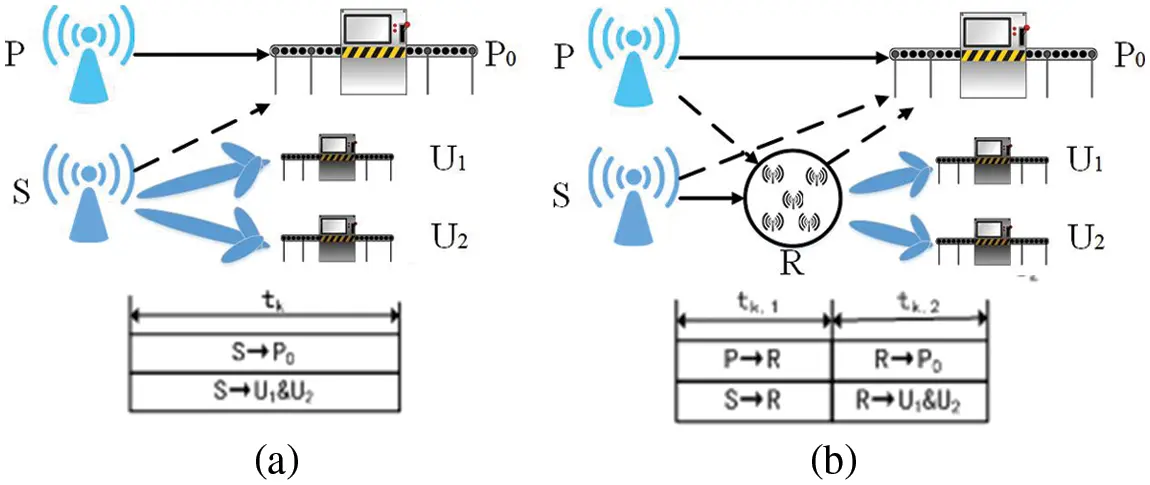
Figure 1: Non-Orthogonal multiple access (NOMA) based cooperative relaying transmission for the industrial Internet of Things (IIoT)
2.1 Protocol Description
Our proposed protocol can be divided into two transmission mechanisms. As shown in Fig. 1a, when the primary monitoring equipment does not exist, S directly transmits data to U1 and U2. Similarly, in Fig. 1b, if the primary monitoring equipment exists, each transmission slot tk is divided into two sub-slots with equal length tk,1 and tk,2. S transmits data to U1 and U2 through the cooperation of relays to expand the transmission range under the constraint of ensuring the Quality of Service (QoS) of the primary monitoring equipment. The time slot structure is analyzed as follows. When the primary monitoring equipment does not exist, S directly transmits data to the destination node. The received signal of U1 and U2 can be written as:
yU1,H0=h1(xreceive)+nSU1,=h1(a1ESx1+a2ESx2)+nSU1,(1)
yU2,H0=h2(xreceive)+nSU2=h2(a1ESx1+a2ESx2)+nSU2.(2)
where h1 and h2 are the transmission channels between the best antennas selected by the antenna selection algorithm AIA-AS. Both nSU1 and nSU2 are the additive white Gaussian noise of monitoring equipment U1 and U2 with variance σ02. ai(i=1,2) is the power allocation coefficient with the condition of a1<a2 and a1+a2=1. When the primary monitoring equipment exists, in the first time slot tk,1, S transmits data to P0 and relay Ri. It is obvious that the primary and secondary transmissions will interfere with each other. So the received signal at Ri and P0 are derived as:
yR,H1=hSRi(xreceive)+σ2=hSRi(a1ESx1+a2ESx2)+EPhPRixP+nSRi,(3)
yP,H1=hSP0(xreceive)+σ2=EPhPP0xP+hSP0(a1ESx1+a2ESx2)+nSP0.(4)
where hSRi is the transmission channel between the optimal antennas selected by the antenna selection algorithm. nSRi, nSP0 are the additive white Gaussian noise of monitoring equipment Ri and P0 with variance σ02.
And all secondary relays decode the signal from S. Those secondary relays that can successfully decode the signal constitute a decoding set Ξ. There are two cases about Ξ in the second time slot.
Case 1: If Ξ is empty (i.e., no relay can successfully decode from S), the direct transmission link is used to retransmit its data to U1 and U2. At the same time, beam-forming technology is used to receive signal from S in order to cancel interference from the primary monitoring equipment at U1 and U2. Then, the received signal at U1 and U2 can be written as:
yU1,H1,Θ=h1(xreceive)+nSU1=h1(a1ESx1+a2ESx2)+nSU1,(5)
yU2,H1,Θ=h2(xreceive)+nSU2=h2(a1ESx1+a2ESx2)+nSU2.(6)
Case 2: If Ξ is not empty, the relay in Ξ that causes the maximum signal-to-noise rate (SNR) of U1, U2 would be selected as the best auxiliary signal transmission. Here, the best relay is expressed as RB. U1 and U2 receive signals from RB by using beam-forming technology. Specifically, U1 and U2 adjust the beam of its antenna pattern aligning with RB, while zero aligns with the primary monitoring equipment. Therefore, interference from the primary monitoring equipment can be restrained to be almost zero. Then, the received signal for U1 and U2 are written as:
yU1,H1=hRU1(xreceive)+nRiU1,=hRU1(a1ESx1+a2ESx2)+nRiU1,(7)
yU2,H1=hRU2(xreceive)+nRiU2=hRU2(a1ESx1+a2ESx2)+nRiU2.(8)
where hRU1 and hRU2 are the transmission channel between the optimal antennas selected by the antenna selection algorithm. nRiU1, nRiU2 are denoted as the additive white Gaussian noise of link RiU1 and RiU2.
2.2 Calculation of Signal-to-Interference-Plus-Noise Ratio (SINR)
Case 1: If the primary monitoring equipment does not exist, S directly transmits data to U1 and U2, then the SINR at the receivers are derived as
γ1→2,H0=a2γS|h1|2×(1+a1γS|h1|2)−1,(9)
γ1,H0=|h1|2×a1γS,(10)
γ2,H0=a2γS|h2|2×(1+a1γS|h2|2)−1.(11)
where γP=EP×(σ02)−1 and γS=ES×(σ02)−1.
Case 2: If the primary monitoring equipment exists, in tk,1, the SINR at Ri are written as:
γSR1=a1γS|hSRi|2×(1+γP|hPRi|2)−1,(12)
γSR2=a2γS|hSRi|2×(1+a1γS|hSRi|2+γP|hPRi|2)−1.(13)
Then, all secondary relays decode the received signal. In tk,2, there are two cases:
If Ξ is empty, S will control the transmit power and retransmit the received signal through the direct link. The SINR of U1 and U2 are given by:
γ1→2,H1=a2γS|h1|2×(1+a1γS|h1|2)−1,(14)
γ1,H1=|h1|2×a1γS,(15)
γ2,H1=a2γS|h2|2×(1+a1γS|h2|2)−1.(16)
If Ξ is not empty, the SINR of U1 and U2 in the second time slot are expressed as:
γ1→2,RU1=a2γUi|hRU1|2×(1=a1γUi|hRU1|2)−1,(17)
γ1,RU1=|hRU1|2×a1γUi,(18)
γ2,RU2=a2γUi|hRU2|2×(1+a1γUi|hRU2|2)−1.(19)
where γUi=ER×(σ02)−1.
2.3 Channel Model
The TWDP fading channel can be described as,
Ph2(γ)=K^2γ¯∑i=1L∑j=01Ciexp(−P2i−j−K^γγ¯)(∑n=0∞1n!2(γP2i−jK^γ¯)n)(20)
where K^=K+1, K is the ratio of total specular power to total diffuse power, P2i=(K^−1)(1+αi), P2i−1=(K^−1)(1−αi), αi=Δcos(π(i−1)/2L−1), Δ is the relative strength of two specular components, Ci is constant coefficient whose length depends on L and the first five exact values are given in [14]. γ¯ is the average SNR, L is the order of probability density function (PDF), Ai,j=P2i−jK^γ/γ¯ and I0 is the modified Bessel function of first kind and zero-th order.
For the convenience of derivation, the definite integral of the PDF of TWDP on the SNR can be expressed as,
∫baPh2(γ)dγ=∫baK^2γ¯∑i=1L∑j=01Ciexp(−P2i−j−K^γγ¯)(∑n=0∞1n!2(P2i−jK^γ¯)nγn)dγ=K^2γ¯∑i=1L∑j=01[Ciexp(−P2i−j)(∑n=0∞1n!2(−P2i−j)n(−exp(−K^γγ¯)n!∑m=0nγmm!(−K^γ¯)m))]|ba(21)
For the convenience of the description, the following formula is defined,
f(a,b,γ¯)=K^2γs∑i=1L∑j=01[Ciexp(−P2i−j)(∑n=0∞1n!2(−P2i−j)n(−exp(−K^aγs)n!∑m=0namm!(−K^γ¯)m+exp(−K^bγs)n!∑m=0nbmm!(−K^γ¯)m))](22)
Next, for the convenience of derivation later, the calculation of g(g1,g2,γp)=∫g1g2Ph2(γ)f(a,b,γs)dγ,γ¯=γp can be expressed as,
g(g1,g2,γ¯2)=∫g1g2Ph2(γ)f(a,b,γ¯1)dγ=∫g1g2K^2γp∑i=1L∑j=01[Ciexp(−P2i−j−K^γγp)(∑n=0∞1n!2(K^P2i−jγpγ)n)]×K^2γs∑c=1L∑d=01[Ccexp(−P2c−d)(∑e=0∞1e!2(−P2c−d)e(−exp(−K^aγs)e!∑h=0eahh!(−K^γs)h+exp(−K^bγs)e!∑k=0ebkk!(−K^γs)k))]=K^24γpγs[∑i=1L∑j=01[Ciexp(−P2i−j)(∑n=0∞1n!2(K^P2i−jγp)n(∑c=1L∑d=01[Ccexp(−P2c−d)(∑e=0∞1e!n−1(−P2c−d)e(η1))]))]]−K^24γpγs[∑i=1L∑j=01[Ciexp(−P2i−j)(∑n=0∞1n!2(K^P2i−jγp)n(∑c=1L∑d=01[Ccexp(−P2c−d)(∑e=0∞1e!n−1(−P2c−d)e(η2))(∑e=0∞1e!n−1(−P2c−d)e(η2))]))]](23)
where,
a=Bγ+C,b=Dγ+E
η1=∑h=0e1h!(−K^γs)hexp(−K^CγS)×∑q=0hexp(−K^γpg1−K^γsg1B)C(q,h)×Bh−q(h+n−q)!∑k=0h+n−q(K^γp+K^γsB)k−h−n+qk!g1kCq(−exp(−(K^γp+K^γsB)g1))−∑h=0e1h!(−K^γs)hexp(−K^EγS)×∑q=0hexp(−K^γpg1−K^γsg1D)C(q,h)×Dh−q(h+n−q)!∑k=0h+n−q(−K^γp−K^γsD)k−h−n+qk!g1kEq
η2=∑h=0e1h!(−K^γs)hexp(−K^CγS)×∑q=0hexp(−K^γpg2−K^γsg2B)C(q,h)×Bh−q(h+n−q)!∑k=0h+n−q(−K^γp−K^γsB)k−h−n+qk!g2kCq−∑h=0e1h!(−K^γs)hexp(−K^EγS)×∑q=0hexp(−K^γpg2−K^γsg2D)C(q,h)×Dh−q(h+n−q)!∑k=0h+n−q(−K^γp−K^γsD)k−h−n+qk!g2kEq(24)
3 Outage Performance Analysis
It is assumed that the time interval of primary transmission defers exponential distribution with μ1, and the duration of primary transmission defers exponential distribution with μ2. The probability that the primary monitoring equipment does not exist can be written as:
Pr{H0}=μ1=μ,(25)
Pr{H1}=μ2=1−μ.(26)
where H0 and H1 are the cases that the primary monitoring equipment does not exist and does exist respectively. When the primary monitoring equipment do not exist, from Eqs. (8)–(10), the outage probability of the secondary monitoring equipment U1 is deduced as:
PoutH0U1=1−Pr{γ1→2,H0>γH0,γ1,H0>γH0}=1−Pr{|h1|2>max(γH0γS(a2−a1γH0),>γH0a1γS)}={f(∞,γH0γS(a2−a1γH0),γsu1),γH0<a2a1<γH0+1f(∞,γH0a1γS,γsu1),a2a1>γH0+1.(27)
The outage probability of the secondary monitoring equipment U2 can be written as:
PoutH0U2=1−Pr{γ2,H0>γH0}=1−Pr{a2γS|h2|21+a1γS|h2|2>γH0}=1−f(∞,γH0a2γS−a1γSγH0,γsu2),a2a1>γH0.(28)
It is assumed that the target rate R1=R2=RR=R∗, when the primary monitoring equipment does not exist, secondary monitoring equipment directly transmit data to the receiver. The target rate can be written as R∗=log2(1+γH0). And the threshold of the direct link can be written as γH0=2R∗−1.
Similarly, when the primary monitoring equipment exists, the secondary monitoring equipment transmits data to the receiver through the cooperation of optimal relay. Therefore, the target rate of the receiver can be expressed as R∗=12log2(1+γH1). Furthermore, the channel transmission threshold can be expressed as γH1=22R∗−1.
PDRi=Pr{γSR1>γH1,γSR2>γH1}=Pr{|hSRi|2>max(γH1(1+γP|hPRi|2)γSa2−a1γSγH1,>γH1(1+γP|hPRi|2)γSa1)}={g(γH1γS(a2−a1γH1),∞,γsr),γH1<a2a1<γH1+1g(γH1γSa1,∞,γsr),a2a1>γH1+1={∫γH1γS(a2−a1γH1)∞Ph2(γ)f(γS(a2−a1γH1)γγH1γP−1γP,0,γpr)dγ,γH1<a2a1<γH1+1∫γH1γSa1∞Ph2(γ)f(γSa1γγH1γP−1γP,0,γpr)dγ,a2a1>γH1+1(29)
when the primary monitoring equipment exists, during the cooperative transmission, Ri decodes the signal x1 and x2. Thus, the probability that Ri can successfully decode the secondary received signal xS during tk,1 is expressed as Eq. (29).
When the primary monitoring equipment exists, the probability of Ξ=Θ and Ξ=Ωl can be written as:
PCΘ=Pr{Ξ=Θ}=∏i=1N(1−PDRi),(30)
PCΩn=Pr{Ξ=Ωn}=∏i∈ΩnPDRi∏j∈Ω¯n(1−PDRi).(31)
Case 1: When the primary monitoring equipment exist, and Ξ is empty, the outage probability of the secondary monitoring equipment U1 is written as:
PoutH1,Θu1=1−Pr{γ1→2,H1>γH1,γ1,H1>γH1}=1−Pr{γH1<min(a2γS,Max|h1|21+a1γS,Max|h1|2,a1γS,Max|h1|2)}=1−Pr{|h1|2>max(γH1γS,Max(a2−a1γH1),γH1a1γS,Max)}={f(∞,γH1γS,Max(a2−a1γH1),γsu1),γH1<a2a1<γH1+1f(∞,γH1a1γS,Max,γsu1),a2a1>γH1+1.(32)
The outage probability of the secondary monitoring equipment U2 is expressed as:
PoutH2,Θu2=1−Pr{γ2,H1>γH1}=1−Pr{a2γS|h2|21+a1γS|h2|2>γH1}=f(∞,γH1a2γS−a1γSγH1,γsu2),a2a1>γH1.(33)
Case 2: When the decoding set Ξ is not empty, S will select the optimal relay RB from Ξ to support the transmission of xS. Here, the optimal relay is the one in Ξ that enables the secondary target monitoring equipment achieving the best outage performance. Therefore, the principle can be expressed as:
RB=argmaxj∈Ωl(min(γ1→2,RjU1,γ1,RjU1,γ2,RjU2)).(34)
From Eqs. (11) to (15), when any one relay Ri in Ξ transmits signal, the outage probability of the secondary monitoring equipment U1 and U2 are written as:
PoutRiu1=1−Pr{a2γS|hRiU1|21+a1γS|hRiU1|2>γH1,a1ρ|hRiU1|2>γH1}={f(∞,γH1a2γS−a1γSγH1,γru1),γH1<a2a1<γH1+1f(∞,γH1a1ρ,γru1),a2a1>γH1+1.(35)
PoutRiu2=1−Pr{γ2,RU2>γH1}=1−Pr{a2γUi|hRU2|21+a1γUi|hRU2|2>γH1}=1−f(∞,γH1a2γUi−a1γH1γUi,γru2),a2a1>γH1(36)
The optimal relay transmission is realized through the selection process of candidate relays. Therefore, the outage probability of the secondary monitoring equipment can be expressed as,
PoutΩnU1=∏Uj∈ΩnPoutRiU1,(37)
PoutΩnU2=∏Uj∈ΩnPoutRiU2.(38)
So, when the primary monitoring equipment exists, the outage probability of secondary transmissions for monitoring equipment is expressed as:
PoutH1U1=PoutH1,ΘU1Pr{Ξ=Θ}+∑n=12N−1PoutΩnU1Pr{Ξ=Ωn},(39)
PoutH1U2=PoutH1,ΘU2Pr{Ξ=Θ}+∑n=12N−1PoutΩnU2Pr{Ξ=Ωn}.(40)
Further, the secondary outage probability of monitoring equipment can be derived as:
PoutU1=PoutH0U1Pr(H0)+PoutH1U1Pr(H1),(41)
PoutU2=PoutH0U2Pr(H0)+PoutH1U2Pr(H1).(42)
Actually, when there is no secondary monitoring equipment in CRN (N=0), Pr{Ξ=Θ}=1 and Pr{Ξ=Ωl}=0. Meantime, if the secondary receiver does not employ beam-forming technology, the monitoring equipment S will control the transmission power and retransmitted signal through the direct link. The SINR of U1 and U2 can be written as:
γ1→2,P=a2γS|h1|2×(1+a1γS|h1|2+γP|hPU1|2)−1(43)
γ1,P=a1γS|h1|2×(1+γP|hPU1|2)−1(44)
γ2,P=a2γS|h2|2×(1+a1γS|h2|2+γP|hPU2|2)−1(45)
Therefore, the traditional secondary outage probability of monitoring equipment can be derived as:
PoutΘu1=1−Pr{γ1→2,P>γH0,γ1,P>γH0}=1−Pr{a2γS|h1|2>max(γH0(a1γS|h1|2+γP|hPU1|2+1),γH0(γP|hPU1|2+1))}={g(γH0γS(a2−a1γH0),∞,γsu1),γH0<a2a1<γH0+1g(γH0γSa1,∞,γsu1),a2a1>γH0+1={∫γH0γS(a2−a1γH0)∞Ph2(γ)f(γS(a2−a1γH0)γγH0γP−1γP,0,γpu1)dγ,γH0<a2a1<γH0+1∫γH0γSa1∞Ph2(γ)f(γSa1γγH0γP−1γP,0,γpu1)dγ,a2a1>γH0+1(46)
PoutΘU2=1−Pr{γ2,P>γH0}=1−Pr{a2γS|h2|2>γH0(a1γS|h2|2+γP|hPU2|2+1)}=1−g(γH0(a2−a1γH0)γS,∞,γsu2)=1−∫γH0(a2−a1γH0)γS∞Ph2(γ)f((a2−a1γH0)γSγγH0γP−1γP,0,γpu2)dγ,a2a1>γH0.(47)
Using Pr{Ξ=Θ}=1 and Pr{Ξ=Ωl}=0 in Eqs. (41) and (42), the outage probability of the conventional principle for monitoring equipment can be concluded.
4 Simulation and Analysis
In this section, the performance of the relay-based NOMA system in the smart factory under different TWDP channel conditions will be simulated and analyzed by matlab, and the outage performance will be evaluated. In order to combine with the monitoring of the production line in the actual factory, we fully considered the interference of the primary monitoring equipment to the secondary transmission network in the simulation test. The system-related parameters are set as follows: The target transmission rate is R∗=0.5b/s/Hz; the power distribution coefficient is a1=0.3, a2=0.7.
In the simulated TWDP channel, we set the channel parameters K and Δ according to the actual situation, where K represents the energy ratio of the two specular reflection components to the scattered components, and Δ represents the intensity difference between the two main path components.
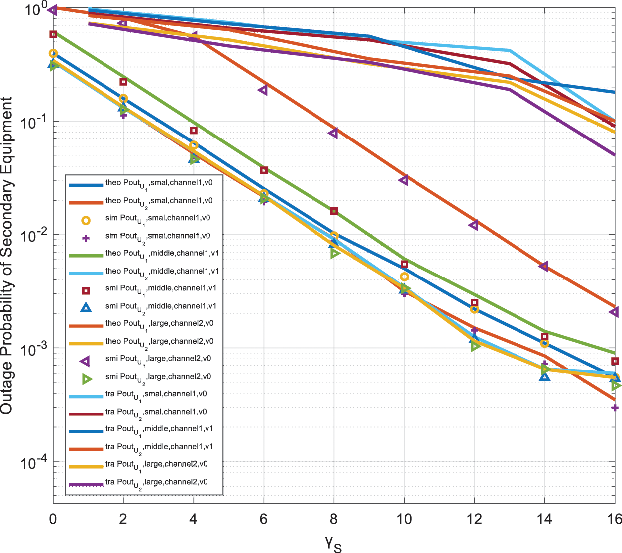
Fig. 2 shows the relationship between the outage probability of the secondary monitoring equipment and the signal-to-noise ratio under different channel conditions of the interference conditions of the primary monitoring equipment. Set the number of relays in the system N=5, SNR of primary monitoring equipment γP=20dB. The simulation results show that, considering the interference factors of the primary monitoring equipment and transmitting through the best relay, the outage probability of secondary system is significantly improved than the traditional mechanism. The secondary network is subject to dual constraints, the QoS of the primary monitoring device and the transmission power of the secondary monitoring device. When the value of ES is small, the power limit of the secondary system greatly affects the outage probability, which will decrease with the increase of γS. When γS increases to a certain extent, the secondary outage probability is mainly affected by the power ES,Max of the monitoring device. In the simulation environment, according to the actual channel existence, we set the channels in four cases, which can be divided into two categories. These two categories contain the intensity difference of the two main path components Δ=0 and Δ=1. In the first type of Δ=0 environment, the channel conditions we set are KSU2=KRU2=0.1, KPR=0.2, KSR=KSU1=KRU1=10, and KSU2=KRU2=1, KPR=2, KSR=KSU1=KRU1=10. In the second type of Δ=1 environment, the channel conditions we set are KSU2=KRU2=0.1, KPR=0.2, KSR=KSU1=KRU1=10 and KSU2=KRU2=1, KPR=2, KSR=KSU1=KRU1=10. It can be seen that, when the intensity difference of the two main path components is particularly large, it is equivalent to when the intensity of one of the two main path components is very low under the condition of Δ=0. Under the condition of Δ=1, the outage probability of the secondary monitoring devices U1 and U2 are both smaller than when the intensity difference between the two main path components is small. When there is only one main path in the channel, the performance of the secondary monitoring equipment of the NOMA system with relay is higher than when there are two main paths in the channel, as the two paths will interfere with each other. Also, it can be seen that when both the channel strength K of U2 and the interference of the primary monitoring equipment increases, the outage probability of primary monitoring equipment can be reduced. Therefore, when the channel conditions of the secondary monitoring equipment improves, the outage probability of the secondary monitoring equipment is significantly reduced.
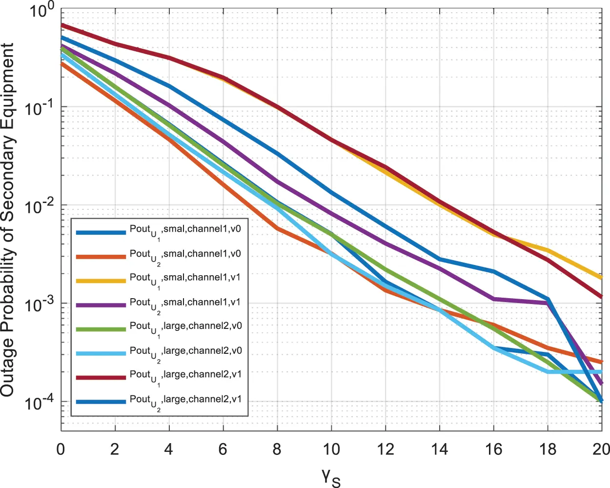
Figure 2: The outage probability of the secondary monitoring equipment, under different channel conditions of the interference conditions of the primary monitoring equipment
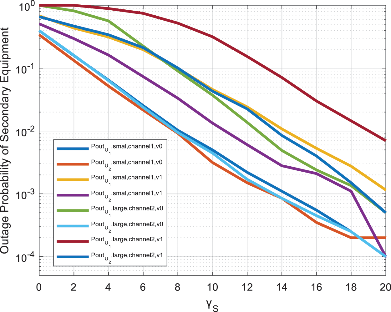
Fig. 3 shows the relationship between the outage probability of the secondary monitoring equipment and the signal-to-noise ratio under different U1 channel environmental conditions. Set the number of relays in the system to N=5, and the signal-to-noise ratio of the primary monitoring equipment γP=20dB. In the simulation environment, according to the actual channel environment, we set the channels in four environments, which can be divided into two categories. These two categories contain the intensity difference of the two main path components Δ=0 and Δ=1, these situations respectively describe the worse or improved overall channel environment. In the first type of Δ=0 environment, the channel conditions we set are KSU2=KRU2=1, KPR=2, KSR=KSU1=KRU1=10 and KSU2=KRU2=10, KPR=20, KSR=KSU1=KRU1=50. In the second type of Δ=1 environment, the channel conditions we set are KSU2=KRU2=1, KPR=2, KSR=KSU1=KRU1=10, and KSU2=KRU2=10, KPR=20, KSR=KSU1=KRU1=50. It can be seen that since the set power distribution coefficient U2 is greater than U1, the outage probability of the secondary monitoring device U2 is lower than that of the monitoring device U1. At the same time, when the environmental strength of one of the two main path components of the TWDP channel is very low, the outage probability of the secondary monitoring equipment basically does not change with the overall improvement of the channel environment. This is due to the influence of the primary monitoring equipment interference on the system. When the overall channel environment is improved, the channel environment interfered by the primary monitoring equipment is also obtained.
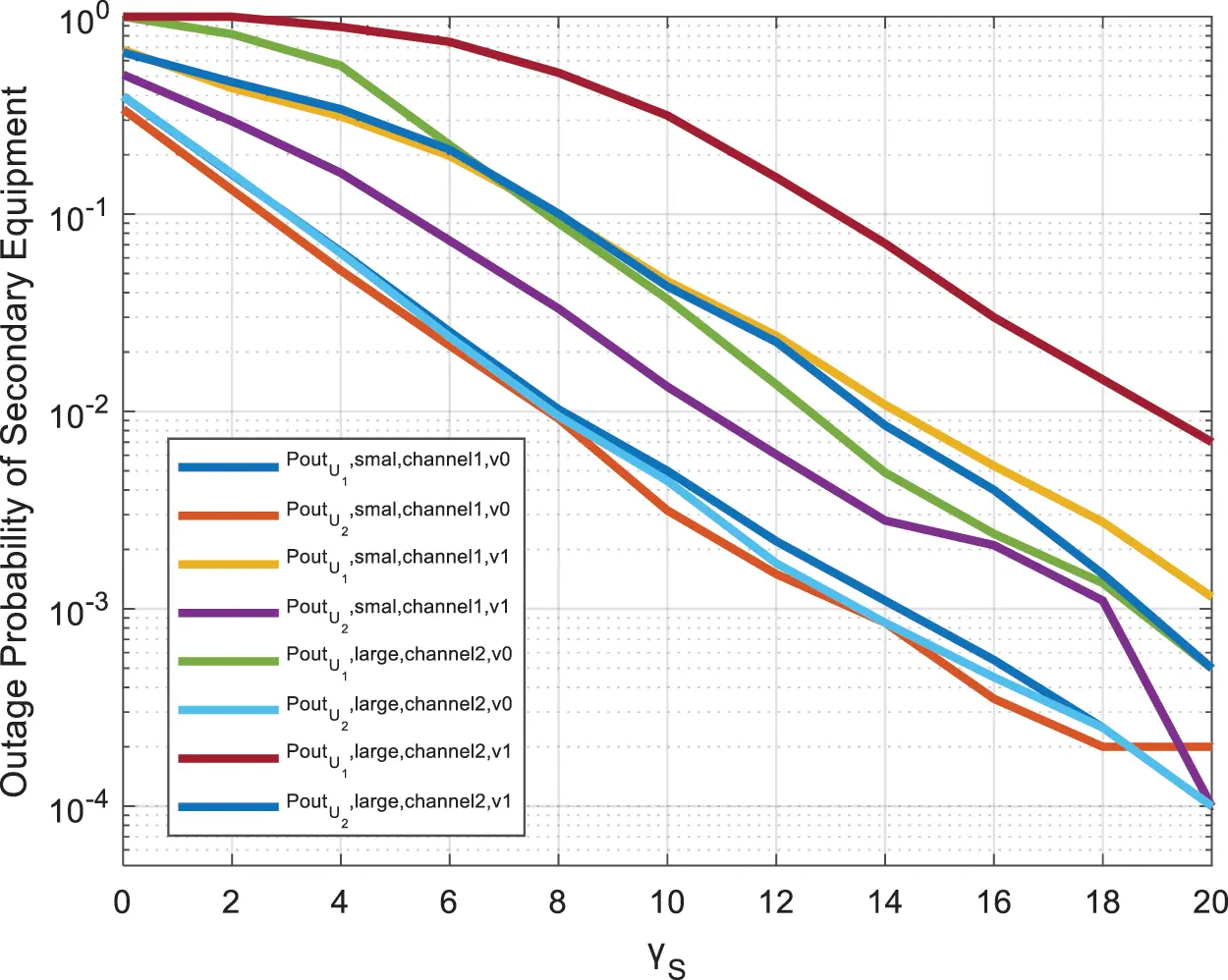
Figure 3: The outage probability of the secondary monitoring equipment, under the conditions of different U1 channel environmental strengths
Fig. 4 shows the relationship between the outage probability of the secondary monitoring equipment and the signal-to-noise ratio under different overall channel environments. Set the number of relays in the system to N=5, and the signal-to-noise ratio of the primary monitoring equipment to γP=20dB. In the simulation environment, we set the channels in three environments according to the actual channel existence. For the fairness of comparison, we set the parameter Δ=0 in the TWDP channel. The channel conditions are set as follows: KSU2=KRU2=1, KPR=2, KSR=KSU1=KRU1=10; KSU2=KRU2=1, KPR=2, KSR=KSU1=KRU1=20 and KSU2=KRU2=1, KPR=2, KSR=KSU1=KRU1=50. It can be seen that the outage probability of the secondary monitoring device U2 is lower than that of the monitoring device U1, indicating that the system performance of U2 is better than that of U1. When the channel conditions of U1 change, the performance of the U2 system basically does not change, and the outage probability of U1 changes with the change of U1 channel strength.
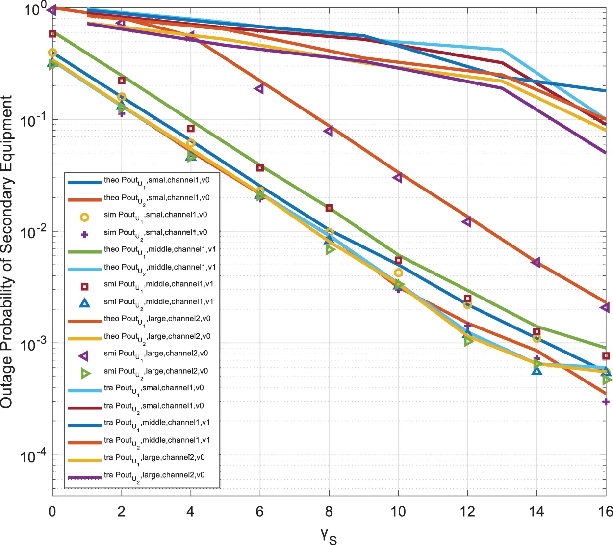
Figure 4: The outage probability of the secondary monitoring equipment, under different overall channel environments
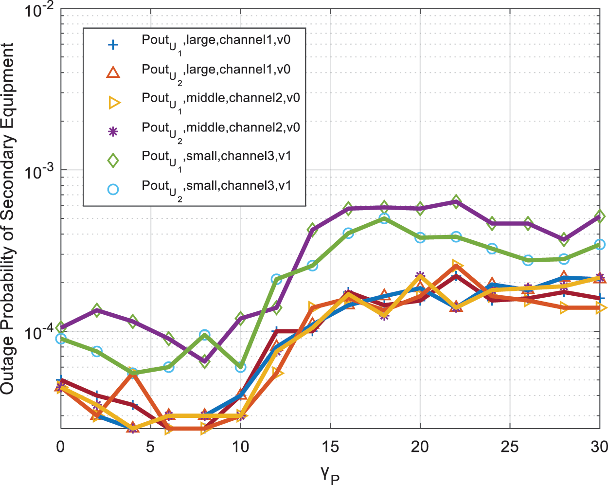
Fig. 5 shows that when the energy ratio K of the two specular reflection components to the scattering component remains unchanged, and the intensity of the two main path components of the channel is very different or not much different, the outage probability of the secondary monitoring device is compared with that of the primary monitoring device. The relationship between the changes in the signal-to-noise ratio. In the system simulation parameters, we set the number of relays in the system to N=3 and the signal-to-noise ratio to γP=20dB. In the simulation environment, we set the channels in the two environments according to the actual channel existence. We set the parameter Δ in the TWDP channel to 0 and 1 respectively in the two channel environments. The channel conditions we set are KSU2=KRU2=1, KPR=2, KSR=KSU1=KRU1=5. It can be seen from the figure that when the two main path components of the TWDP channel are very different, it is equivalent to only one main channel in the channel. At this time, U1 and U2 show interruption due to the difference in channel environment and power allocation. Outage performance of U1 is slightly better than U2. When the difference between the two main path components of the TWDP channel is not very large, the power distribution coefficient has a dominant influence on the system performance. At this time, the outage probability performance of U2 is significantly better than that of U1. Also, when there are two main path components in the channel, the system can be damaged, and the performance is lower than when there is only one main path component in the TWDP channel.
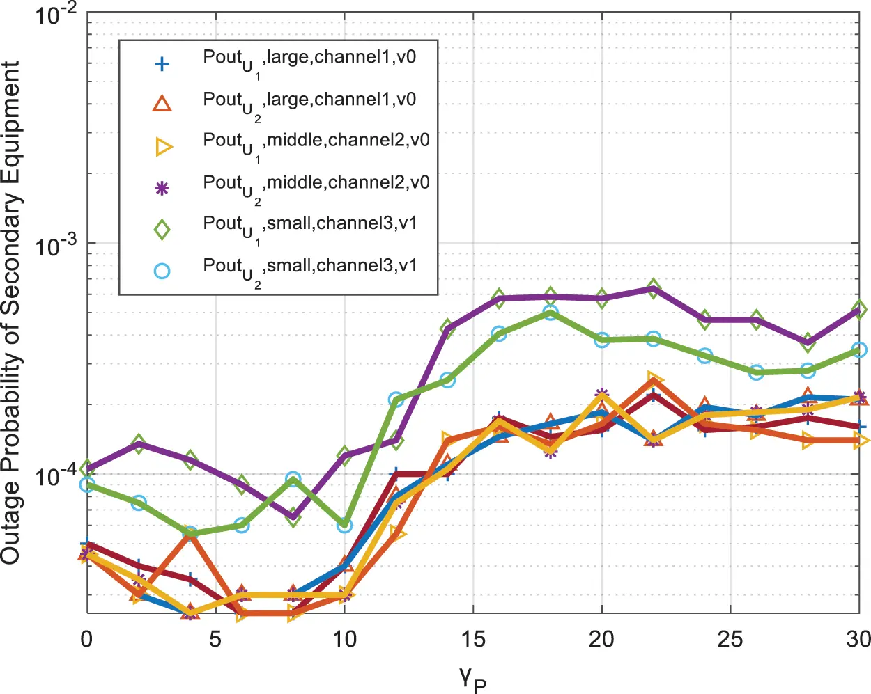
Figure 5: The outage probability of the secondary monitoring equipment under different K channel environments
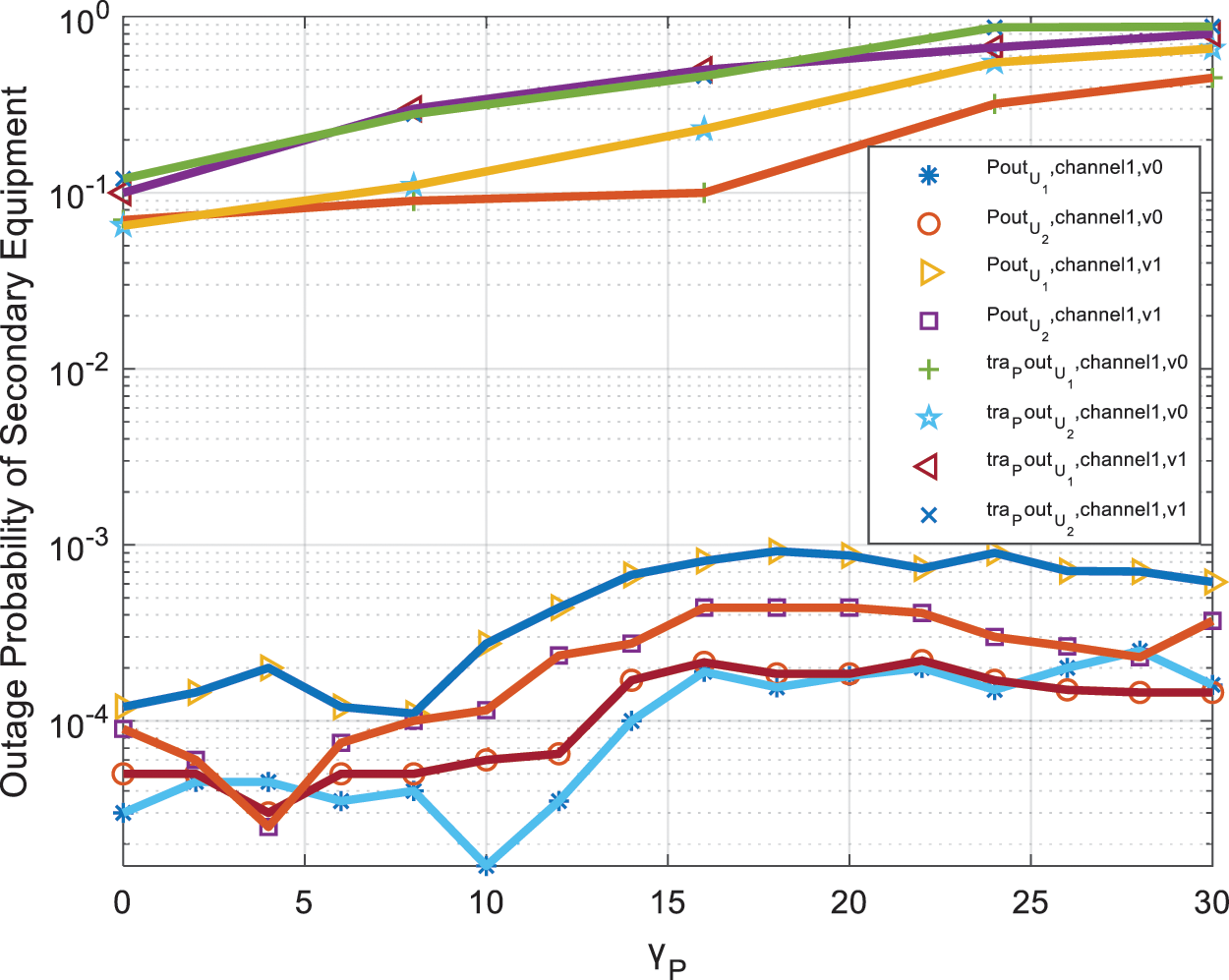
Fig. 6 shows the relationship between the outage probability of the secondary monitoring device and the signal-to-noise ratio of the primary monitoring device when the U1 channel environment changes greatly. In the system simulation parameters, we set the number of relays in the system to N=3 and the signal-to-noise ratio to γP=20dB. In the simulation environment, we set the channels in three environments according to the actual channel existence. We set the parameter Δ=0 or Δ=1 in the TWDP channel. The channel conditions are set as follows: KSU2=KRU2=1, KPR=2, KSR=KSU1=KRU1=2.3, Δ=1; KSU2=KRU2=1, KPR=2, KSR=KSU1=KRU1=2.5, Δ=0 And KSU2=KRU2=1, KPR=2, KSR=KSU1=KRU1=3, Δ=0. It can be seen from the figure that when the two main path components of the TWDP channel are not much different, the performance of the outage probability of the secondary monitoring devices U1 and U2 is not as good as when there is only one main path component in the TWDP channel. At the same time, it can be seen that when the channel condition of the monitoring device U1 improves, the outage probability of U1 performs well than when the channel environment is poor.

Figure 6: The outage probability of the secondary monitoring equipment when the U1 channel environment changes greatly
5 Conclusions
In this article, in order to use IIoT technology to monitor the factory assembly line, and solve the problem of secondary transmission interruption caused by frequent occupation of authorized spectrum by primary equipment in the TWDP channel environment, we propose an improved spectrum sharing mechanism based on beam-forming, optimal relay selection, power control and NOMA Access mechanism. The mechanism is suitable for system transmission under the TWDP channel, ensuring the continuity of secondary transmission and reducing the possibility of secondary interruption while ensuring that the primary user is hardly affected. In addition, in this paper, we derive the outage probability of the improved mechanism in the TWDP channel environment and compare it with the traditional mechanism. Finally, the simulation results confirmed that compared with the traditional mechanism, the mechanism significantly improves the performance of the secondary transmission in the TWDP channel environment. Though the improvement of secondary transmission is achieved at the cost of frequent occupation of authorized spectrum of primary equipment and the introduction of relays cause an increase in the complexity of hardware, the proposed transmission mechanism can guarantee the continuity of the secondary transmission, greatly reduce the outage probability of the secondary transmission, and improve the efficiency of the factory’s monitoring of the production line. However, there are still some technical issues to be solved, such as the compatibility of NOMA with 5G, the design issues of various NOMA techniques for user separation, etc. The future research will focus on these directions.
Funding Statement: This work is supported by Sichuan Science and Technology Program (NO.2020YFG0321), Standard Development and Test bed Construction for Smart Factory Virtual Mapping Model and Digitized Delivery (No. MIIT 2019–00899–3–1) and Tianjin Intelligent Factory based on Industrial Internet Digital Twin Platform (No. 20201030).
Conflicts of Interest: The authors declare that they have no conflicts of interest to report regarding the present study.
References
1. N. Panwar, S. Sharma and A. K. Singh, “A survey on 5G: The next generation of mobile communication,” Physical Communication, vol. 18, no. 2, pp. 64–84, 2016. [Google Scholar]
2. J. Thompson, H. C. Ge and R. Irmer, “5G wireless communication systems,” American Journal of Engineering Research (AJER), vol. 2, no. 10, pp. 344–353, 2013. [Google Scholar]
3. J. Wurm, K. Hoang, O. Arias, A. R. Sadeghi and Y. Jin, “Security analysis on consumer and industrial IoT devices,” in 2016 21st Asia and South Pacific Design Automation Conf. (ASP-DAC), Macao, China, IEEE, pp. 519–524, 2016. [Google Scholar]
4. C. Jiang, C. Wei, T. Fei and L. Chun, “Industrial IoT in 5G environment towards smart manufacturing,” Journal of Industrial Information Integration, vol. 10, pp. 10–19, 2018. [Google Scholar]
5. Q. Wang, X. Zhu, Y. Ni, L. Gu and H. Zhu, “Blockchain for the IoT and industrial IoT: A review,” Internet of Things, vol. 10, pp. 100081.1–100081.9, 2020. [Google Scholar]
6. B. Chen, J. Wan, S. Lei, L. Peng and B. Yin, “Smart factory of industry 4.0: Key technologies, application case, and challenges,” IEEE Access, vol. 6, pp. 6505–6519, 2017. [Google Scholar]
7. Z. Qu, J. Keeney, S. Robitzsch, F. Zaman and X. Wang, “Multilevel pattern mining architecture for automatic network monitoring in heterogeneous wireless communication networks,” China Communications, vol. 13, no. 7, pp. 108–116, 2016. [Google Scholar]
8. A. Daniel, K. Baalamurugan, V. Ramalingam and K. Arjun, “Energy aware clustering with multihop routing algorithm for wireless sensor networks,” Intelligent Automation & Soft Computing, vol. 29, no. 1, pp. 233–246, 2021. [Google Scholar]
9. S. Wang, J. Wan, D. Li and C. Zhang, “Implementing smart factory of industrie 4.0: An outlook,” International Journal of Distributed Sensor Networks, vol. 12, no. 1, pp. 3159805.1–3159805.10, 2016. [Google Scholar]
10. I. Budhiraja, N. Kumar, S. Tyagi, S. Tanwar and D. Y. Suh, “A systematic review on NOMA variants for 5G and beyond,” IEEE Access, vol. 9, pp. 85573–85644, 2021. [Google Scholar]
11. Z. Ding, Y. Liu, J. Choi, Q. Sun, M. Elkashlan et al., “Application of non-orthogonal multiple access in LTE and 5G networks,” IEEE Communications Magazine, vol. 55, no. 2, pp. 185–191, 2017. [Google Scholar]
12. Y. Zhang, J. Liu, Y. Peng, Y. Dong and C. Zhao, “Performance analysis of intelligent CR-NOMA model for industrial IoT communications,” Computer Modeling in Engineering & Sciences, vol. 125, no. 1, pp. 239–257, 2020. [Google Scholar]
13. Y. Huang, C. Zhang, J. Wang, Y. Jing, L. Yang et al., “Signal processing for MIMO-NOMA: Present and future challenges,” IEEE Wireless Communications, vol. 25, no. 2, pp. 32–38, 2018. [Google Scholar]
14. Z. Ding, L. Dai and H. V. Poor, “MIMO-NOMA design for small packet transmission in the internet of things,” IEEE Access, vol. 4, pp. 1393–1405, 2016. [Google Scholar]
15. H. B. Chikha and A. Almadhor, “Automatic classification of superimposed modulations for 5G mimo two-way cognitive relay networks,” Computers, Materials & Continua, vol. 70, no. 1, pp. 1799–1814, 2022. [Google Scholar]
16. S. Alabed, I. Maaz and M. Al-Rabayah, “Improved bi-directional three-phase single-relay selection technique for cooperative wireless communications,” Computers, Materials & Continua, vol. 70, no. 1, pp. 999–1015, 2022. [Google Scholar]
17. A. Shah, M. S. Islam and M. S. Alam, “Cooperative communication in wireless networks,” IEEE Communications Magazine, vol. 42, no. 10, pp. 74–80, 2004. [Google Scholar]
18. Y. Na, J. Jung, Y. You and H. Song, “Adaptive relay selection scheme for minimization of the transmission time,” Computers, Materials & Continua, vol. 69, no. 1, pp. 1361–1373, 2021. [Google Scholar]
19. A. Azarfar, J. Frigon and B. Sanso, “Improving the reliability of wireless networks using cognitive radios,” IEEE Communications Surveys & Tutorials, vol. 14, no. 2, pp. 338–354, 2011. [Google Scholar]
20. D. Dixit and P. R. Sahu, “Performance of QAM signaling over TWDP fading channels,” IEEE Transactions on Wireless Communications, vol. 12, no. 4, pp. 1794–1799, 2013. [Google Scholar]
Appendix
The derivation of the f function is as follows:
∫baPh2(γ)dγ=∫baK^2γ¯∑i=1L∑j=01Ciexp(−P2i−j−K^γγ¯)(∑n=0∞1n!2(P2i−jK^γ¯)nγn)dγ=K^2γ¯∑i=1L∑j=01∫baCiexp(−P2i−j−K^γγ¯)(∑n=0∞1n!2(P2i−jK^γ¯)nγn)dγ=K^2γ¯∑i=1L∑j=01∫baCiexp(−P2i−j)(∑n=0∞1n!2(P2i−jK^γ¯)nγne−K^γγ¯)dγ=K^2γ¯∑i=1L∑j=01∫baCiexp(−P2i−j)(∑n=0∞1n!2(P2i−jK^γ¯)nγne−K^γγ¯)dγ
As ∫xne−xdx=−e−xn!∑k=0nxkk!+C, where C is an arbitrary constant. So we can get,
∫baPh2(γ)dγ=K^2γ¯∑i=1L∑j=01[Ciexp(−P2i−j)(∑n=0∞1n!2(−P2i−j)n(−exp(−K^γγ¯)n!∑m=0nγmm!(−K^γ¯)m))]|ba
The derivation of the g function is as follows:
g(g1,g2,γ¯2)=∫g1g2Ph2(γ)f(a,b,γ¯1)dγ=∫g1g2K^12γp∑i=1L∑j=01[Ciexp(−P2i−j−K^1γγp)(∑n=0∞1n!2(K^1P2i−jγpγ)n)]×K^22γs∑c=1L∑d=01[Ccexp(−P2c−d)(∑e=0∞1e!2(−P2c−d)e(−exp(−K^2aγs)e!∑h=0eahh!(−K^2γs)h+exp(−K^2bγs)e!∑k=0ebkk!(−K^2γs)k))]dγ=K^1K^24γpγs∫g1g2{[e−K^1γγp1n!2(K^1P2i−jγpγ)n×∑c=1L∑d=01[Ccexp(−P2c−d)×(∑e=0∞1e!2(−P2c−d)e(−exp(−K^2aγs)e!∑h=0eahh!(−K^2γs)h+exp(−K^2bγs)e!∑k=0ebkk!(−K^2γs)k))]]∑i=1L∑j=01[Ciexp(−P2i−j)[∑n=0∞[e−K^1γγp1n!2(K^1P2i−jγpγ)n×∑c=1L∑d=01[Ccexp(−P2c−d)×(∑e=0∞1e!2(−P2c−d)e(−exp(−K^2aγs)e!∑h=0eahh!(−K^2γs)h+exp(−K^2bγs)e!∑k=0ebkk!(−K^2γs)k))]][e−K^1γγp1n!2(K^1P2i−jγpγ)n×∑c=1L∑d=01[Ccexp(−P2c−d)×(∑e=0∞1e!2(−P2c−d)e(−exp(−K^2aγs)e!∑h=0eahh!(−K^2γs)h+exp(−K^2bγs)e!∑k=0ebkk!(−K^2γs)k))]]]]}dγ=K^1K^24γpγs∫g1g2{∑i=1L∑j=01[Ciexp(−P2i−j)[∑n=0∞[e−K^1γγp1n!2(K^1P2i−jγpγ)n×∑c=1L∑d=01[Ccexp(−P2c−d)×(∑e=0∞1e!2(−P2c−d)e(−exp(−K^2aγs)e!∑h=0eahh!(−K^2γs)h+exp(−K^2bγs)e!∑k=0ebkk!(−K^2γs)k))]][1n!2(K^1P2i−jγp)n×∑c=1L∑d=01[Ccexp(−P2c−d)×(∑e=0∞e!e!2(−P2c−d)e(−∑h=0eexp(−K^2aγs)e−K^1γγp(γ)nahh!(−K^2γs)h+∑k=0eexp(−K^2bγs)e−K^1γγp(γ)nbkk!(−K^2γs)k))]]]]}dγ=K^1K^24γpγs∫g1g2{∑i=1L∑j=01[α[∑n=0∞[β×∑c=1L∑d=01[δ(∑e=0∞ϕ(−∑h=0eexp(−K^2aγs)e−K^1γγp(γ)nahh!(−K^2γs)h+∑k=0eexp(−K^2bγs)e−K^1γγp(γ)nbkk!(−K^2γs)k)(−∑h=0eexp(−K^2aγs)e−K^1γγp(γ)nahh!(−K^2γs)h+∑k=0eexp(−K^2bγs)e−K^1γγp(γ)nbkk!(−K^2γs)k))]]]]}dγ
In order to facilitate the derivation of the subsequent formula, we have defined the following variables. These variables are not a function of the signal-to-noise ratio and do not affect the integrality of derivation.
α=Ciexp(−P2i−j)β=1n!2(K^1P2i−jγp)nδ=Ccexp(−P2c−d)ϕ=1e!(−P2c−d)e
Then we can get that,
∫g1g2−∑h=0eexp(−K^2aγs)e−K^1γγp(γ)nahh!(−K^2γs)h+∑k=0eexp(−K^2bγs)e−K^1γγp(γ)nbkk!(−K^2γs)kdγ=∫g1g2−∑h=0eexp(−K^2(Bγ+C)γs)e−K^1γγp(γ)n(Bγ+C)hh!(−K^2γs)h+∑k=0eexp(−K^2(Dγ+E)γs)e−K^1γγp(γ)n(Dγ+E)kk!(−K^2γs)kdγ=∫g1g2−∑h=0e1h!(−K^2γs)he−K^2Cγs(Bγ+C)hexp(−K^2Bγγs)e−K^1γγp(γ)n+∑k=0e1k!(−K^2γs)ke−K^2Eγsexp(−K^2Dγγs)e−K^1γγp(γ)n(Dγ+E)kdγ=∫g1g2−∑h=0e1h!(−K^2γs)he−K^2Cγse(−K^1γp−K^2Bγs)γ(γ)n[λ(0,h)Bhγh+λ(1,h)Bh−1γh−1C1+…]+∑k=0e1k!(−K^2γs)ke−K^2Eγse(−K^1γp−K^2Dγs)γ(γ)n[λ(0,h)Dhγh+λ(1,h)Dh−1γh−1E1+…]dγ
where λ(1,h) represents the combined formula. We define that p1=K^1γp+K^2γsB,p2=K^1γp+K^2γsD, then we can get that,
∫g1g2−∑h=0e1h!(−K^2γs)he−K^2Cγse(−K^1γp−K^2Bγs)γ(γ)n[λ(0,h)Bhγh+λ(1,h)Bh−1γh−1C1+…]+∑k=0e1k!(−K^2γs)ke−K^2Eγse(−K^1γp−K^2Dγs)γ(γ)n[λ(0,h)Dhγh+λ(1,h)Dh−1γh−1E1+…]dγ=∫g1g2−∑h=0e1h!(−K^2γs)he−K^2Cγse−p1γ(p1γ)n1(p1)n∑q=0h(λ(q,h)Bh−q(p1γ)h−qCq1(p1)h−q)+∑k=0e1k!(−K^2γs)ke−K^2Eγse−p2γ(p2γ)n1(p2)n∑q=0h(λ(q,h)Dh−q(p1γ)h−qEq1(p2)h−q)dγ=∫g1g2−∑h=0e1h!(−K^2γs)he−K^2Cγs1(p1)n∑q=0h(λ(q,h)Bh−qe−p1γ(p1γ)n+h−qCq1(p1)h−q)+∑k=0e1k!(−K^2γs)ke−K^2Eγs1(p2)n∑q=0h(λ(q,h)Dh−qe−p2γ(p2γ)n+h−qEq1(p2)h−q)dγ
And ∫xne−xdx=−e−xn!∑k=0nxkk!+C. So the result of the final integration can be deduced as,
∫g1g2−∑h=0e1h!(−K^2γs)he−K^2Cγs1(p1)n∑q=0h(λ(q,h)Bh−qe−p1γ(p1γ)n+h−qCq1(p1)h−q)+∑k=0e1k!(−K^2γs)ke−K^2Eγs1(p2)n∑q=0h(λ(q,h)Dh−qe−p2γ(p2γ)n+h−qEq1(p2)h−q)dγ=−∑h=0e1h!(−K^2γs)he−K^2Cγs∑q=0h(Cqλ(q,h)Bh−q(p1)h−q+n(−e−p1γ(h+n−q)!×∑z=0h+n−q(p1γ)zz!))+∑k=0e1k!(−K^2γs)ke−K^2Eγs∑q=0h(Eqλ(q,h)Dh−q(p2)h−q+n(−e−p2γ(h+n−q)!×∑z=0h+n−q(p2γ)zz!))+Q
Q is an arbitrary constant in the above formula. Finally we can get the deduced result as follows.